A Theoretical Framework to Derive Simple, Firing-Rate-Dependent Mathematical Models of Synaptic Plasticity
 Janne Lappalainen
 Juliane Herpich1,2
  Christian Tetzlaff
- 1Department of Computational Neuroscience, Third Institute of Physics-Biophysics, Georg-August-University, Göttingen, Germany
- 2Bernstein Center for Computational Neuroscience, Georg-August-University, Göttingen, Germany
Synaptic plasticity serves as an essential mechanism underlying cognitive processes as learning and memory. For a better understanding detailed theoretical models combine experimental underpinnings of synaptic plasticity and match experimental results. However, these models are mathematically complex impeding the comprehensive investigation of their link to cognitive processes generally executed on the neuronal network level. Here, we derive a mathematical framework enabling the simplification of such detailed models of synaptic plasticity facilitating further mathematical analyses. By this framework we obtain a compact, firing-rate-dependent mathematical formulation, which includes the essential dynamics of the detailed model and, thus, of experimentally verified properties of synaptic plasticity. Amongst others, by testing our framework by abstracting the dynamics of two well-established calcium-dependent synaptic plasticity models, we derived that the synaptic changes depend on the square of the presynaptic firing rate, which is in contrast to previous assumptions. Thus, the here-presented framework enables the derivation of biologically plausible but simple mathematical models of synaptic plasticity allowing to analyze the underlying dependencies of synaptic dynamics from neuronal properties such as the firing rate and to investigate their implications in complex neuronal networks.
1. Introduction
Synaptic plasticity serves as an essential mechanism of neuronal networks being linked to diverse functional properties such as the cognitive mechanisms of learning and memory (Hebb, 1949; Martin et al., 2000). Amongst others, to understand the details of this link between synaptic plasticity and functional properties of a neuronal system, theoretical or mathematical models of synaptic plasticity are formulated and investigated (Dayan and Abbott, 2001; Gerstner et al., 2012, 2014). On the one hand, detailed biological models of synaptic plasticity are formulated closely related to experiments, which provide molecular details or synaptic dynamics given diverse stimulation protocols (Earnshaw and Bressloff, 2006; Graupner and Brunel, 2010; Graupner and Brunel, 2012; Antunes et al., 2016; Gallimore et al., 2018). However, to capture the richness of the underlying molecular processes and to match a wide repertoire of experimental findings, the resulting theoretical models become mathematically rather complex and often depend on detailed spike-timings, which impedes further analysis especially on the neuronal network level. On the other hand, to investigate the link between synaptic plasticity and functional properties of neuronal systems, compact, simple theoretical models of synaptic plasticity are developed neglecting the underlying biological details (Tsodyks and Feigelman, 1988; Gerstner and Kistler, 2002; Tetzlaff et al., 2011, 2013; Knoblauch and Sommer, 2016). In contrast to the spike-dependency of the detailed models, these compact models usually depend on the average firing rates of neurons (Gerstner and Kistler, 2002). However, the detailed formulation of these compact models are rather phenomenological and they are only loosely linked to the detailed biological models.
Here, we will provide a mathematical method enabling us to derive a compact, firing-rate-dependent theoretical model from a biologically detailed spike-based model. For the detailed model, we consider two versions of a well-established calcium-based spike-timing-dependent plasticity model (Graupner and Brunel, 2012; Graupner et al., 2016; Li et al., 2016). We will show that this model can be simplified such that the general dynamics induced by it can be well-described by a compact, rate-dependent model.
Many experimental studies have been performed to investigate the multiplicity of molecular processes, which are involved in synaptic plasticity. Thereby, calcium currents are identified as key players of at least two molecular processes that mediate the change in synaptic strength by synaptic plasticity (Kandel et al., 2000; Lüscher and Malenka, 2012; Korte and Schmitz, 2016). First, inside the cell, calcium triggers different pathways resulting to changes in the number and phosphorylation of AMPA receptors yielding the potentiation (strengthening) and depression (weakening) of synapses (Choquet and Triller, 2013; Huganir and Nicoll, 2013). The second process is triggered by endocannabinoids and induces depression of synapses (Sjöström et al., 2001; Sjöström et al., 2003; Nevian and Sakmann, 2006). The endocannabinoids are transmitted retrogradely from the postsynaptic neuron to the presynaptic neuron changing the neurotransmitter release capability. For this, calcium plays a crucial role (Hashimotodani et al., 2005; Maejima, 2005). These molecular findings are integrated into a theoretical model, in which the postsynaptic calcium concentration within the dendritic spine directly accounts for synaptic plasticity (Graupner and Brunel, 2012). The calcium concentration, in turn, is modulated by spike-dependent pre- and postsynaptic processes. This calcium-dependent model matches several experimental findings and represents a biologically detailed theoretical model of synaptic plasticity.
After introducing our mathematical method to derive compact models from detailed models (see section 2), we simplify the calcium-dependent model of synaptic plasticity to derive a compact model with synaptic changes dependent on pre- and postsynaptic firing rates. We repeat this procedure for different versions of the considered synaptic plasticity model as well as neuron model. For all cases, the resulting compact model reliably matches the dynamics of the detailed model indicating that, despite the mathematical simplification, the compact model captures the essentials of synaptic dynamics. Further analyses of the resulting compact models reveal, amongst others, that the dynamics of synaptic plasticity are dominated by the square of the presynaptic firing rate, which is in contrast to phenomenologically derived compact theoretical models. Thus, the here developed method enables the derivation of simple, compact, and rate-dependent models from detailed ones allowing further investigations on the network level without loss of essential details of the synaptic dynamics.
2. Materials and Methods
In this study, we derive a simplified, compact, firing-rate-dependent mathematical formulation of the detailed dynamics of spike-timing dependent plasticity. For this, we analyze the firing rate dependency of the detailed model and, based on this, estimate the functional relations between activity and synaptic weight changes by regression analysis. As detailed model, we consider a well-established calcium-based synaptic plasticity model, which describes a multitude of plasticity effects based on the underlying molecular dynamics of calcium currents in the postsynaptic dendritic spine (Graupner and Brunel, 2012; Graupner et al., 2016). To take the influence of network effects and postsynaptic activity dynamics into account, we focus in our analysis on three fundamental network motifs. These motifs consist of one or two different presynaptic neuronal populations connected to one postsynaptic neuron. In the following, first, we introduce the different considered motifs and the detailed models of synaptic plasticity as well as used neuron models (please see Table 1 for used parameter values). Then, we describe our generic approach to investigate the firing rate dependencies of synaptic plasticity to derive a simplified, compact mathematical description.
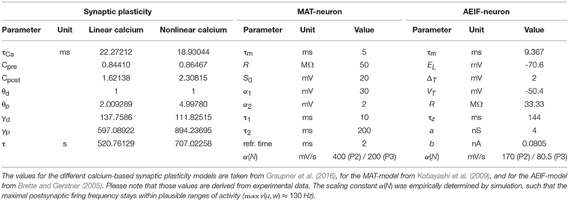
Table 1. Used values for model parameters.
2.1. Neuronal Setups
Throughout this study we consider three basic neuronal motifs or setups: a presynaptic population with independent postsynaptic neuron (P1; Figure 1, top left), a presynaptic population with dynamic postsynaptic neuron (P2; Figure 1, top middle), and two presynaptic populations with dynamic postsynaptic neuron (P3; Figure 1, top right).
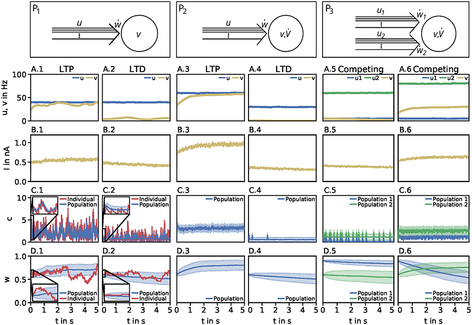
Figure 1. Dynamics of the detailed model of calcium-based synaptic plasticity for three different neuronal setups P1, P2, and P3. The different setups are shown schematically in the first row. The following rows show (second row; A) the average firing rates, (third row; B) the postsynaptic input current, (fourth row; C) the calcium concentration of an individual synapse using the LC-model (red) and population average (blue) with standard deviation (blue shading), and (fifth row; D) the synaptic weight of an individual synapse (red) and population average (blue) with standard deviation (blue shading). Columns 1 and 2: Dynamics of the P1-setup for initial synaptic strengths of w(t0) = 0.6 and pre- and postsynaptic spike-firing of u = v = 40Hz (column 1; LTP) and u = 40Hz and v = 5Hz (column 2; LTD). Columns 3 and 4: Same as in columns 1 and 2 for the P2-setup with presynaptic spike-firing of u = 60Hz (column 3; LTP) and u = 30Hz (column 4; LTD). Columns 5 and 6: Same as in previous columns for P3-setup of two, competing presynaptic populations 1 (blue) and 2 (green) with initial synaptic weights of w1(t0) = 0.9, w2(t0) = 0.6 and presynaptic spike-firing of u1 = 5Hz, u2 = 60Hz (column 5; no competition) and u1 = 5Hz, u2 = 80Hz (column 6; strong competition). In all cases the populations consist of N = 1, 000 synapses. The continuous presynaptic activities were obtained by averaging all N spiketrains and temporally filtering with an alpha function window of 100ms width. The postsynaptic activities were obtained with an alpha function window of 500ms width and using the MAT-model. The calcium and current traces were filtered with a moving average of 25ms width.
Neuronal Population I (P1): This motif consists of one population of N = 1, 000 presynaptic neurons (single lines abstracted to one arrow) connected to one postsynaptic neuron (circle). All presynaptic neurons fire independently from each other by a Poisson process with frequency u. The postsynaptic neuron is active by a Poisson process with frequency v. Note, in this setup the firing of the postsynaptic neuron is independent of the activity of the presynaptic population, since all spike trains are generated independently by probabilistic Poisson processes. These processes can yield, at a specific point in time, different synaptic weights for different presynaptic neurons. Thus, we consider the average synaptic strength of the presynaptic population denoted by w.
Neuronal Population I with neuron model (P2): This setup is similar to the P1-setup. However, here, the activity of the postsynaptic neuron is not determined by a Poisson process (see P1), instead, we consider a biologically detailed neuron model. For generality, throughout this study we use two different neuron models; the so-called Multi-timescale Adaptive Threshold model (MAT; Kobayashi et al., 2009) and the Adaptive Exponential Integrate-and-Fire model (AEIF; Brette and Gerstner, 2005). Thus, the activity of the presynaptic population can influence the firing of the postsynaptic neuron. Consequently, the change in the postsynaptic firing rate () depends on u and w, i.e., , which in turn influences the dynamics of synaptic plasticity (ẇ).
Neuronal Population II (P3): This motif is an extension of the P2-setup. Here, two presynaptic populations 1 and 2 are connected to the same postsynaptic neuron with each population consisting of independently firing neurons with population-specific frequency u1 and u2, respectively. Thus, the firing of the postsynaptic neuron depends on the presynaptic firing rates and strength of the connecting synapses of both presynaptic populations (). Note, the only difference between both populations is the firing frequency, as all other parameters are set to be the same. Consequently, we only investigate the influence of the firing rate of the first population as results also hold for the second population.
2.2. Calcium-Based Synaptic Plasticity Model
The strength of an individual synapse connecting a presynaptic neuron i with the postsynaptic one, denoted by ρi, underlies the following dynamic (Graupner and Brunel, 2012;Graupner et al., 2016):
The first term describes the processes of long-term potentiation (LTP) at a synapse with γp being the rate of synaptic increase, θp being the potentiation threshold. ci(t) is the activity-dependent postsynaptic calcium-concentration, which is described either by a linear calcium model (LC; see section 2.2.1) or a more complex nonlinear calcium model (NLC; see section 2.2.2). H(x) denotes the Heaviside function. Analogously, the second term describes the processes of long-term depression (LTD) at a synapse in accordance to the parameters γd and θd.
The noise term accounts for coincidental activity-dependent dynamics and non-plasticity related weight dynamics and is given by
where τ is the same temporal constant as in Equation 1, σ is a constant amplitude parameter, and ηi(t) represents Gaussian white noise with mean zero and unit variance drawn for each synapse individually.
2.2.1. Linear Calcium Dynamics (LC)
In the linear calcium (LC) model, the dynamics of the intracellular calcium concentration of the postsynaptic spine for each synapse, denoted as , is given by:
where τCa is the time constant of the calcium decay. The calcium concentration increases with pre- and postsynaptic spike times and tl of amplitudes Cpre and Cpost, respectively. Delays between spiking events and the flow of ions are neglected as such delays only shift the independent, probabilistic spike events in the time domain. Please note, instead of Equation 3, we also consider a more complex set of equations to model the calcium dynamics as described in the following.
2.2.2. Nonlinear Calcium Dynamics (NLC)
In the nonlinear calcium (NLC) model, the calcium concentration ci(t) = ci, pre(t) + ci, post(t) is determined by presynaptically evoked transients of calcium, described by
and postsynaptically evoked transients of calcium given by
where the quantities τCa, , tl, Cpre and Cpost are analog to the linear calcium model. The nonlinearity factor
couples the pre- and postsynaptic calcium concentrations (Graupner et al., 2016).
2.3. Neuron Model
2.3.1. Multi-Timescale Adaptive Threshold Neuron (MAT)
The multi-timescale adaptive threshold (MAT) model (Kobayashi et al., 2009; Yamauchi et al., 2011) describes the postsynaptic membrane potential as a leaky integrator:
where τm is the membrane time constant, R the membrane resistance, and I the excitatory postsynaptic current. The excitatory postsynaptic current provides the linkage to the calcium-based plasticity model by summing the incoming spikes dependent on the synaptic weights:
N denotes the size of the presynaptic population, ρi the synaptic strength connecting the presynaptic neuron i to the postsynaptic neuron, the presynaptic spiking times, and α(N) is a population-size-dependent scaling constant for the current.
After each postsynaptic spike time tj, the spiking threshold S gets adapted by
with S0 being the resting threshold. The update of the threshold and its decay is described by multiple timescales, τ1 and τ2, and amplitudes, α1 and α2, and is given by
2.3.2. Adaptive Exponential Integrate-and-Fire Neuron (AEIF)
The adaptive exponential integrate-and-fire (AEIF) model (Brette and Gerstner, 2005) describes the postsynaptic membrane potential as
where is the membrane time constant composed of the membrane capacitance C and the leak conductance gL, EL is the leak reversal potential, VT the spiking threshold, ΔT a slope factor, I the excitatory postsynaptic current as given in Equation 8, and z is the adaptation current determined by
Here, τz denotes the adaptation time constant and a the subthreshold adaptation. Once a spike is triggered, the variable z is increased by an amount b which denotes the spike-triggered adaptation and V is reset to the reset potential Vr = EL.
2.4. Acquisition of Data, Transformation, and Analysis
The acquisition of the data resulting from the detailed model and its transformation to an activity-dependent, compact model of synaptic plasticity is carried out in a similar manner for all three different neuronal setups, two plasticity, and two neuron models. In the following, the corresponding steps taken are explained (Figure 2).
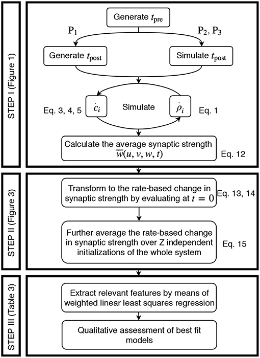
Figure 2. Generic approach to derive the firing rate dependencies of calcium-based STDP. Step I involves the simulation of the detailed calcium-based STDP model. Step II transforms the data obtained in Step I to rate-dependent data of synaptic plasticity. In Step III the rate-dependent data is analyzed using a regression algorithm and the results are evaluated.
Step I: Simulation of Calcium-Based STDP.
We solve the differential equations of synaptic (and neuronal) dynamics numerically by the Euler method with time step Δt = 0.5 ms for different presynaptic input frequencies. The parameter space of the system is given by the presynaptic firing frequency u (and postsynaptic activity v for P1) between 0 and 100 Hz (with a step size of 1 Hz) and the initialization of the synaptic strength w(t0) between 0 and 1 (in arbitrary units) with a step size of 0.05. Please see Table 2 for an overview of the analyzed parameter spaces. An exemplary time evolution of the involved quantities is shown in Figure 1 for the LC-model (section 2.2.1) with the MAT neuron model (section 2.3.1). Due to the fast time constant for the calcium concentration (τCa), the calcium concentration is initialized at zero.
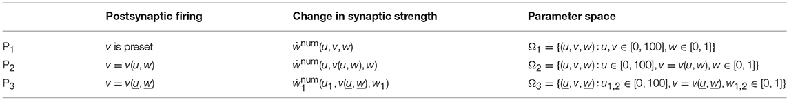
Table 2. Mathematical notations for the different neuronal setups.
As the activities drive the change of synaptic weights, given each pair of pre- and postsynaptic spike train, we calculate the average synaptic strength () of all synapses (ρi) across a period of two seconds:
where N is the size of the presynaptic population and ρi is given by solving Equation 1 with corresponding calcium dynamics numerically. Alongside, the numerical simulation yields the activity of the postsynaptic neuron. The latter is preset for P1 or calculated as spike count over 500 ms for P2 and P3, denoted as v(u, w) for P2 and for the P3-setup (here indicates a vector). However, the resulting is analyzed further in Step II described next.
Step II: Transformation to Rate-Based Data for Synaptic Plasticity.
The mean synaptic strength from the numerical solution of the detailed synaptic plasticity model is further approximated by cubic splines to . By this, the result is regularized from random fluctuations and enables us to calculate a reliable numerical derivative at the initial point in time. This approximation is described by
where Spline is the UnivariateSpline function in the python library scipy.interpolate with parameters k and s. Here, k is the degree of the smoothing spline and s specifies the number of knots. The routine increases the number of knots until the smoothing condition is satisfied.
By considering the synaptic dynamics only around the first time point t = 0, on the one hand, the direct time-dependency is eliminated and, on the other hand, the weight-dependency of synaptic plasticity becomes controllable by neglecting its long-term development. Instead, we scan the weight-dependency of the weight change by considering different initial values for w. Thus, the change in synaptic strength of the population can be expressed as:
Please note that the resulting does not significantly depend on the initial distribution of ρi (see Figure S1). We average the change in synaptic strength of the population over several statistically independent initializations z (total number of intializations Z = 100 for P1, P2 and Z = 38 for P3) of the same parameter set. By this, we obtain the final overall change in synaptic strength (from numerics)
In case of P3, in which we consider two independent presynaptic populations, thus, v(u1, u2, w1, w2), we add indices in order to differentiate between both populations such that
describe the change of the average synaptic strength of population 1 and 2, respectively. As mentioned before, in the P3-setup both populations dynamics are similar. Therefore, we will only consider the weight changes and variables related to the first population, if not stated otherwise.
In summary, based on these definitions for all neuronal setups (Table 2), the (average) synaptic weight changes of the detailed model ẇ commonly depends on the average population firing rate u, the postsynaptic firing rate v, and the average synaptic strength w, which are all local variables of synaptic plasticity (Gerstner and Kistler, 2002).
Step III: Regression Analysis.
Given the transformation of the numerical data from spike-dependencies to firing rate dependencies (Step II), in the following, we fit our rate-based data of synaptic changes ẇnum(u, v, w) by regression analysis to obtain compact mathematical formulations of the underlying weight dynamics. Thus, we will obtain a function of the form of
with i being the postsynaptic and j the presynaptic neuron.
To obtain such a function, we fit the rate-dependent data (Step II) by a Taylor series expansion containing combinations of the involved state variables u, v, w (for better readability we omit the neuronal indices) with coefficients cαβγ. The indices α, β, and γ indicate the order of the state variables u, v, and w in the corresponding feature uαvβwγ:
Here, we limit the amount of considered features (individual terms) to the 27 listed in Table 4 to reduce the number of possible combinations for the regression analysis. These are all features with α, β, γ ∈ {0, 1, 2}; thus, individual state variables of these features are maximally of the second order. The choice of the second order is related to general rate-based equations used in literature, such as the Hebb rule (Hebb, 1949), the Oja rule (Oja, 1982), or the BCM rule (Bienenstock et al., 1982). In all these equations, no quantity is higher than the second order (Tetzlaff et al., 2011). Of course, higher orders or rather more features can be considered if required.
The regression algorithm, we use, is a weighted linear least squares regression and thus minimizes the weighted sum of squared residuals. The weights are inferred from the variance across the results from the Z independent initializations. As a measure of accuracy, the weighted coefficient of determination (R2) was determined from 5-fold cross-validation. Note that it was further unbiased with respect to the number of considered features (Theil, 1958; Willett and Singer, 1988).
Qualitative Analysis of Resulting Compact Models
From the procedure described above we obtain a compact model consisting of a simplified differential equation, which resembles the dynamics of the corresponding complex model. However, to provide a better understanding of the underlying properties of the resulting compact models, we will assess whether these fulfill several qualitative characteristics of synaptic plasticity identified from numerical results (here we focus on the LC-model). For this, we define nine different qualitative characteristics, which are provided in the following. Please note that these characteristics are defined such that a compact model can either fulfill them or not.
1. LTP Area: If the average synaptic weight is below a certain value, essentially for all combinations of pre- and postsynaptic frequencies, LTP dominates the synaptic changes. The LTP Area weight value is about 0.3 (ẇ(w) > 0 for w > 0.3).
2. LTD Increase: If the synaptic weight is between the LTP Area weight value and the equilibrium value of the synaptic dynamics (w*), the influence of LTD on the synaptic dynamics increases with larger weight values which, in turn, decreases the overall influence of LTP with LTP still being the dominant process (ẇ > 0 with ẇ(w1) > ẇ(w2) for w1 < w2).
3. LTD Area: If the synaptic weight is above the equilibrium value w*, LTD dominates the synaptic weight dynamics for all combinations of pre- and postsynaptic frequencies (ẇ(w) < 0 for w > w*).
4. Invariability: If the pre- and postsynaptic activities are below 10 Hz, synaptic changes become negligible (ẇ ≈ 0 for u, v < 10).
5. Curvilinearity: For increasing pre- and/or postsynaptic activities (above 10 Hz), ẇ(u, v) switches from a convex function to a concave function.
6. Saturation: For high levels of neuronal activity, synaptic changes (ẇ) become independent of the actual frequency of neuronal activities.
7. w-Behavior: For the P1-setup, the change of synaptic weights depends linearly on the actual synaptic weight (ẇ(w) ≈ w). For the P2- and P3-setup, ẇ(w) has one maximum.
8. Competition: (Only for the P3-setup) If one population is highly active, the connections from the second to the postsynaptic neuron experience depression via competition.
9. Steadiness: (Only for the P3-setup) If the activity of one population approaches a maximum level, the influence of the other population on the system dynamics is negligible.
3. Results
In this study, we develop a simple, compact mathematical model by inferring the neuronal firing rate dependency of synaptic plasticity from a detailed, calcium-based synaptic plasticity model (Graupner and Brunel, 2012; Graupner et al., 2016). For this, we consider three different neuronal setups of one (P1, P2) or two (P3) presynaptic neuronal population(s) connected onto one postsynaptic neuron and analyze the dependencies of synaptic changes (ẇ) on the (average) pre- and postsynaptic neuronal activities (u, v) and the corresponding synaptic weight (w). For generality, we consider two different models of synaptic plasticity and two different neuron models (see section 2). In other words, for a given neuron model, plasticity model, and neuronal setup, first, we simulate the dynamics of the detailed plasticity model given different levels of pre- and postsynaptic activities. Then, we transfer the data from spiking-based to rate-based and, finally, fit the activity-dependencies by regression analysis. This analysis provides the synaptic changes given different terms or features of pre-, postsynaptic activity, and the synaptic weight and is repeated for other combinations of models and setups. For details please see section 2. Please note that, in the following, we will focus on synaptic plasticity with linear calcium dynamics (LC-model; section 2.2.1) with the MAT neuron model (section 2.3.1) to explain the basics of our approach and results.
We restricted the regression analysis by considering maximal second order terms resulting in 27 different features of u, v, w each individually weighted (see Table 4 for all considered features). Thus, for all neuronal setups, we searched for the most relevant combinations of 27 features that fit best the simulation-based dependencies evaluated by calculating the coefficient of determination between fit and simulation data from 5-fold cross-validation in the four-dimensional space of ẇ, w, u, v (see Figure 3A for different intersections). The resulting best fits serve as reference estimator of the corresponding setup. The reference estimators reached accuracies of R2 = 0.981 for the P1-setup (Figures 3 A.1,A.2,C.1), R2 = 0.986 for the P2-setup (Figures 3 A.3,A.4,C.2), and R2 = 0.963 for the P3-setup (Figures 3A.5,A.6,C.3). To compare the resulting estimators more qualitatively with the simulation data, we defined nine characteristics of the simulated synaptic weight changes and analyzed whether the resulting estimators or compact models match these (see Material and Methods and Table 3). The reference estimators meet all characteristics (except Saturation and, additionally, Steadiness in P3) and, thus, the reference estimators basically describe the dynamics of the detailed, calcium-based synaptic dynamics. However, common simple models of synaptic plasticity consist of a small number of individual terms (Gerstner and Kistler, 2002; Tetzlaff et al., 2011; Gerstner et al., 2014). Thus, we repeated the regression analysis searching for the combination of three features fitting best the data (Figure 3B) and compared the most accurate three-feature-estimators with the corresponding reference estimator. As expected, the lower number of considered features fits the data less accurate (see Figure 3C), however, the resulting differences remain quantitative (large values of R2) and qualitative small (compare Figure 3B with A).
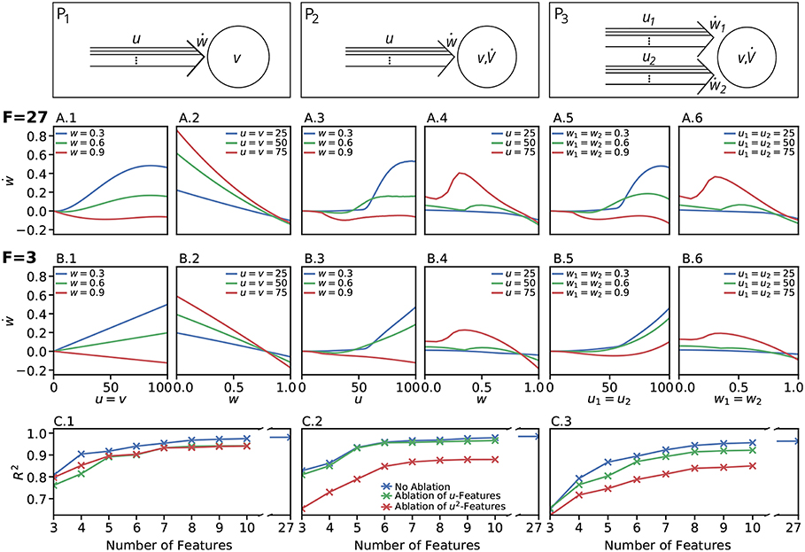
Figure 3. Firing rate-dependent synaptic plasticity dynamics for the three different neuronal setups P1 (left) P2 (middle), and P3 (right). Data for the LC-model with the MAT neuron model are shown. (A) Activity-based change in synaptic strength for the reference fit with 27 features (F = 27) for predefined initial synaptic weights (odd panels) and neuronal activities (even panels) for each neuronal setup, respectively. Deviations from simulated data are negligible. (B) Same as in (A) for the best model with three features (F = 3). (C) For a wide variety of number of features the corresponding models (indicated by the coefficient of determination R2) match the simulated data describing the dependencies of synaptic weight changes on activities and current weight.
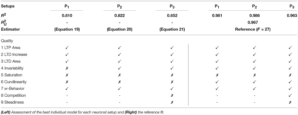
Table 3. Assessment of best fit models with nine qualitative characteristics.
In more detail, starting with the P1-setup consisting of one presynaptic population connected to a postsynaptic neuron of clamped activity, the most accurate three-feature-estimator (Figures 3B.1,B.2) is given by
with an accuracy of R2 = 0.810 (with weighting cαβγ of feature uαvβwγ; , , ). This model fulfills all linear and nonlinear characteristics except the nonlinear characteristics of Invariability, Saturation, and Curvilinearity (Table 3).
Next, the most accurate three-feature-estimator for the P2-setup (Figures 3B.3,B.4), which is a presynaptic population connected to a postsynaptic neuron with dynamic postsynaptic activity, is
with an accuracy of R2 = 0.822 (with , , ) and fulfilling the majority of the characteristics correctly except Saturation and Curvilinearity (Table 3). Finally, the best three-feature-estimator for the P3-setup (Figures 3B.5,B.6), which is similar to the P2-setup except that it consists of two presynaptic populations, is given by
with an accuracy of R2 = 0.652 (with , , ) and depicts five of nine characteristics correctly (all except Saturation, Curvilinearity, Steadiness, and Competition; Table 3).
Although the three-feature-estimators do not match the nonlinear aspects (e.g., Curvilinearity) of the detailed synaptic plasticity dynamics, the resulting rules (Equations 19–21) reliably match the basics of synaptic plasticity, for instance the regimes of LTP and LTD. Thus, they are representing simple, compact mathematical models of synaptic plasticity specifically for each setup.
Given the different models with numbers of features ranging from three to ten (Figure 3C), we analyzed the consistency of each feature within all the eight best estimators per setup to derive which features are generally powerful in describing synaptic plasticity. For the P1-setup, the accuracies of these estimators range from 0.810 for three features to 0.975 for ten features (Figure 3C.1). For the setups P2 and P3, the accuracies lie in [0.822, 0.979] and [0.652, 0.956], respectively (Figures 3C.2,C.3).
Next, we repeated these analyses for all models and derived the absolute frequency for each feature occurring in the eight best estimators (Table 4). For the P1-setup the most frequently occurring features are uv, uw and vw. The Hebbian correlation terms (uv and uvw) are also often present in the P2- and P3-setup. Interestingly, besides the Hebbian terms, for all setups and models, the u2- and u2w-feature occur frequently. This suggests that the square of the presynaptic firing rate is an important component influencing synaptic weight dynamics. To verify this finding, we excluded all features having a u2-term and derived new estimators. These estimators match the data from the detailed model less accurately (red in Figure 3C) than the estimators with u2-terms (blue). Note that, if for instance all terms being linear in u are excluded (green), the R2-values of the resulting estimators are similar to the complete estimators emphasizing the importance of the u2-terms. Thus, we conclude a general trend toward a significant correlation between synaptic plasticity and the square of presynaptic activity, which is not often considered in literature.
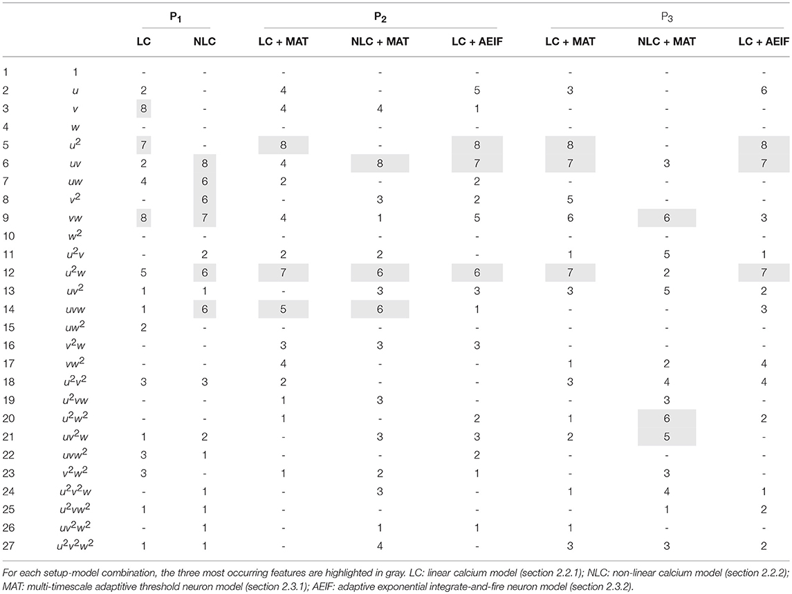
Table 4. Number of occurrences of each feature for the eight best estimators for each setup and different models.
After deriving the best compact model for each setup (Equations 19–21), next, we will derive the model which most precisely describes synaptic plasticity regarding all three different neuronal setups. For that purpose we are focusing on the LC-model with the MAT neuron model. We consider a unified accuracy measure being the mean over all individual accuracies minus their standard deviation. Subtracting the standard deviation is meant to avoid a bias with respect to a certain setup.
In the following, we will discuss the three most accurate unified estimators resulting from this analysis (Table 5): The first most accurate unified estimator is
with , , . Please note that the cαβγ-values for all unified estimators are derived from a 5-fold cross-validation across all setups and models.
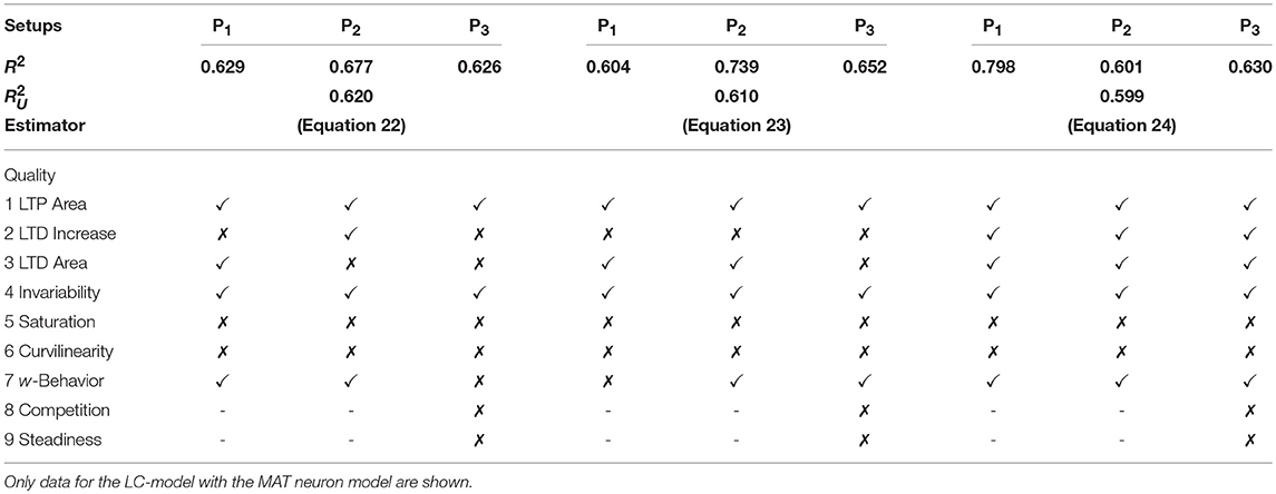
Table 5. Assessment of the best three unified models describing the collective dynamics of all three neuronal setups with nine qualitative characteristics.
The second estimator is
with , , . Both estimators or models contain the features u2, u2v and only differ slightly in their stabilizing features u2w and u2w2 (c201, c202 < 0). Quantitatively, they best match the neuronal setup P2. Qualitatively, they fail in correctly describing several characteristics of synaptic plasticity (Table 5).
On the other hand, the third most accurate unified estimator contains Hebbian terms (uv and uvw) as well as a stabilizing one uw2 with c102 < 0:
with , , . Interestingly, this estimator matches best the P1-setup and it qualitatively generalizes better than the two most accurate unified estimators. It also correctly depicts diverse characteristics of synaptic plasticity. In addition, this estimator best captures the dynamics considering the nonlinear calcium dynamics (Table 6). We simulated the activity-dependent synaptic plasticity dynamics of this estimator (compact model) and compared it with the detailed, calcium-dependent model for the different setups using the LC-model with MAT neuron model (Figure 4). Overall, the compact model matches the dynamics of the complex model especially in the long-term dynamics for LTP as well as LTD. Thus, the long-term dynamics of the rate-based model converge to the synaptic value of spike-timing-dependent plasticity.
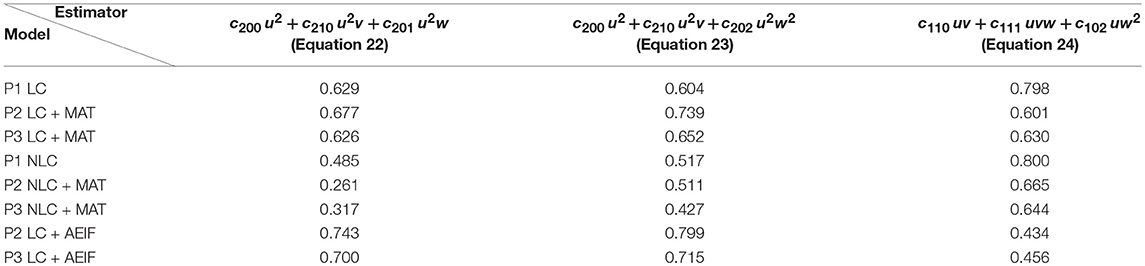
Table 6. R2-values for the unified estimators across all models.
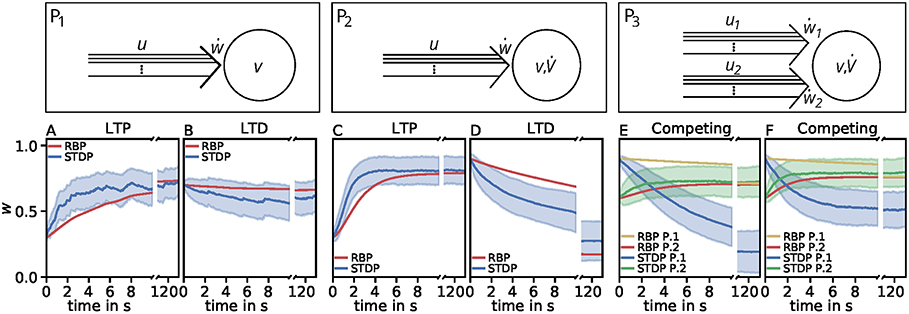
Figure 4. Comparison of spike-timing dependent synaptic plasticity with rate-based synaptic plasticity according to the third unified estimator (Equation 24). Here, we show the results using the LC-model with the MAT neuron model. (A,B): Dynamics of P1 for global initial synaptic strengths of w = 0.3 and pre- and postsynaptic spike-firing of u = v = 35Hz (A; LTP) and w = 0.7 and u = v = 20Hz (B; LTD). The rate-based plasticity (RBP) is illustrated in red whereas the average spike-timing dependent plasticity (STDP) is illustrated in blue. (C,D) Same as in (A,B) for P2 with global initial synaptic strengths of w = 0.3 and presynaptic spike-firing of u = 65Hz (C; LTP) and w = 0.9 u = 36Hz (D; LTD). The rate-based plasticity (RBP) is illustrated in red whereas the average spike-timing dependent plasticity (STDP) is illustrated in blue. (E,F) Same as in C,D for competitive behavior in P3 of two presynaptic populations 1 (blue) and 2 (green) with initial synaptic weights of w1 = 0.9, w2 = 0.6 and presynaptic spike-firing of u1 = 5Hz, u2 = 75Hz (E; no competition) and u1 = 5Hz, u2 = 90Hz (F; strong competition). The rate-based plasticities for populations 1 and 2 are illustrated in yellow and red respectively. The corresponding average spike-timing dependent plasticity is illustrated in blue and green. In all cases the populations consist of N = 1, 000 synapses.
However, the effect of competition between two neuronal populations is not well matched by the simple rate-based model (Figures 4E,F). If we allow a fourth feature in the estimator, the resulting compact model describes competition, too (Figure 5). This is also an example indicating that, if a specific property of the detailed model is desired, one has to consider more features to obtain a compact model which also includes this property. Similarly, if a compact model is desired which matches more accurate the detailed model, more features have to be incorporated (see e.g., Figure 3C).
Figure 5. Comparison of spike-timing dependent synaptic plasticity with rate-based synaptic plasticity according to the third unified estimator (Equation 24) with the additional feature vw2. As in Figure 4, we show the results using the LC-model with the MAT neuron model. (A,B): Dynamics of P1 for global initial synaptic strengths of w = 0.3 and pre- and postsynaptic spike-firing of u = v = 35Hz (A; LTP) and w = 0.7 and u = v = 20Hz (B; LTD). The rate-based plasticity (RBP) is illustrated in red whereas the average spike-timing dependent plasticity (STDP) is illustrated in blue. (C,D) Same as in (A,B) for P2 with global initial synaptic strengths of w = 0.3 and presynaptic spike-firing of u = 65Hz (C; LTP) and w = 0.9 u = 36Hz (D; LTD). The rate-based plasticity (RBP) is illustrated in red whereas the average spike-timing dependent plasticity (STDP) is illustrated in blue. (E,F) Same as in (C,D) for competitive behavior in P3 of two presynaptic populations 1 (blue) and 2 (green) with initial synaptic weights of w1 = 0.9, w2 = 0.6 and presynaptic spike-firing of u1 = 5Hz, u2 = 75Hz (E; no competition) and u1 = 5Hz, u2 = 90Hz (F; strong competition). The rate-based plasticities for populations 1 and 2 are illustrated in yellow and red respectively. The corresponding average spike-timing dependent plasticity is illustrated in blue and green. In all cases the populations consist of N = 1, 000 synapses.
In summary, our results lead to the conclusion that features of squared presynaptic activity are well describing and likely be associated to synaptic plasticity. Nevertheless, the third unified estimator (Equation 24) provides evidence that models of other features exist that better describe the qualitative linear characteristics of synaptic plasticity throughout different neuronal setups while they quantitatively perform worth.
4. Discussion
We developed a method to derive a simple, compact mathematical model of synaptic plasticity based on a biologically detailed, calcium-based model. In contrast to the detailed model, the resulting simple model can be used for further analytical and/or numeric analysis of, for instance, large-scale systems.
An alternative method is, for instance, to derive the cross-correlation function of neuronal firing (Brunel and Hakim, 1999; Ostojic et al., 2009) and, then, to incorporate this function into a mean-field model of synaptic plasticity (Kempter et al., 1999). This method is mathematically more accurate as our method and it can also be used to investigate the self-organization of neural circuits (Ocker et al., 2015; Tannenbaum and Burak, 2015). However, deriving the cross-correlation function of neuronal firing or the mean-field model of synaptic plasticity for diverse detailed neuron and plasticity models is very complex and, up to now, not always possible. On the other hand, the complexity of our method depends less on the considered neuron and synaptic plasticity models.
We considered two different versions of the calcium-based STDP model with parameters which where determined by Graupner et al. (2016) on slices of the visual cortex from macaque monkeys. Of course, these parameters (and also from the neuron model) could vary for different brain regions. However, with the here-developed method one can easily link these parameters to simpler models of plasticity. Given that the function of a brain region is mainly determined on the network level, by using the resulting simple model one can investigate the influence of the parameters on the functional properties of the brain regions.
Overall, we cannot guarantee that we applied the optimal weighting of the observations and thus found the best linear unbiased estimator. Technically, it could be checked if the whole covariance matrix of the N observations in Z initializations would provide a better weighting. However, this is computationally not feasible, especially for the case of P3 with 4.5 Mio. observations. Furthermore, we considered the estimators or models with the highest R2 while taking the next best model into account could yield other reasonable learning rules matching, for instance, more qualitative characteristics (see for instance Equation 24). If a compact model is required, which matches the detailed model with a higher accuracy, instead of three features, one can easily allow more features being present in the final estimator (Figure 3C). Furthermore, by considering features of higher order than two in Step III, the resulting final estimators could describe additional aspects of the detailed model. However, given the increased number of features, the regression procedure would require more computational resources.
The results for individual learning rules of the considered neuronal populations did not significantly match with, for instance, the BCM (Bienenstock et al., 1982) or the Oja's rule (Oja, 1982). Although the results significantly match Hebbian correlation learning, the stabilization mechanisms are different to commonly used ones. Overall, regarding the treated rate-based models, our applied methods on three different neuronal setups suggest that features from the BCM rule and Oja's rule are not the best estimators for the underlying plasticity data. From our methods, features observed to be correlated to LTP are the Hebbain term uv and terms, which depend on the square of the presynaptic activity such as u2v (opposing to v2w from BCM theory) and u2. Features observed to be correlated to LTD are vw, u2w (opposing to v2w from Oja's rule), and uvw. The u2-terms could imply that, on the network level, synaptic dynamics are more sensitive to variations in the inputs (u) than in the network activity (v) providing a stronger influence of the actual inputs on the overall network dynamics. However, such dynamics and the u2-dependency require further theoretical and experimental studies. For instance, by varying systematically the rate of stimulation triggering synaptic plasticity (similar to Sjöström et al., 2001), the resulting ẇ-u-relation could indicate a u2-dependency. Overall, the plausibility of certain terms remain unclear and corresponding molecular pathways of synaptic plasticity still have to be investigated to find pieces of evidence for these terms. However, on the one hand, our method provides a way to link complex synaptic plasticity dynamics with dynamics on the network level and, on the other hand, the individual terms from our method allow to identify important ingredients of synaptic plasticity enabling an (functional) ordering of diverse molecular pathways.
Author Contributions
CT study design. JL data acquisition. JL, JH, and CT data analysis and manuscript written.
Funding
The research was funded by the H2020-FETPROACT project Plan4Act (#732266) (JH and CT), by the Collaborative Research Center SFB-1286 (Project C1) (CT), and by the International Max Planck Research School for Physics of Biological and Complex Systems by stipends of the country of Lower Saxony with funds from the initiative Niedersächsisches Vorab and of the University of Göttingen (JH).
Conflict of Interest Statement
The authors declare that the research was conducted in the absence of any commercial or financial relationships that could be construed as a potential conflict of interest.
Acknowledgments
We acknowledge support by the German Research Foundation and the Open Access Publication Funds of the Göttingen University.
Supplementary Material
The Supplementary Material for this article can be found online at: https://www.frontiersin.org/articles/10.3389/fncom.2019.00026/full#supplementary-material
References
Antunes, G., Roque, A. C., and Simoes-de Souza, F. M. (2016). Stochastic induction of long-term potentiation and long-term depression. Sci. Rep. 6:30899. doi: 10.1038/srep30899
Bienenstock, E. L., Cooper, L. N., and Munro, P. W. (1982). Theory for the development of neuron selectivity: orientation specificity and binocular interaction in visual cortex. J. Neurosci. 2, 32–48. doi: 10.1523/JNEUROSCI.02-01-00032.1982
Brette, R., and Gerstner, W. (2005). Adaptive exponential integrate-and-fire model as an effective description of neuronal activity. J. Neurophysiol. 94, 3637–3642. doi: 10.1152/jn.00686.2005
Brunel, N., and Hakim, V. (1999). Fast global oscillations in networks of integrate-and-fire neurons with low firing rates. Neural Comput. 11, 1621–1671. doi: 10.1162/089976699300016179
Choquet, D., and Triller, A. (2013). The dynamic synapse. Neuron 80, 691–703. doi: 10.1016/j.neuron.2013.10.013
Earnshaw, B. A., and Bressloff, P. C. (2006). Biophysical model of AMPA receptor trafficking and its regulation during long-term potentiation/long-term depression. J. Neurosci. 26, 12362–12373. doi: 10.1523/JNEUROSCI.3601-06.2006
Gallimore, A. R., Kim, T., Tanaka-Yamamoto, K., and De Schutter, E. (2018). Switching on depression and potentiation in the cerebellum. Cell Rep. 22, 722–733. doi: 10.1016/j.celrep.2017.12.084
Gerstner, W., and Kistler, W. M. (2002). Mathematical formulations of Hebbian learning. Biol. Cybern. 87, 404–415. doi: 10.1007/s00422-002-0353-y
Gerstner, W., Kistler, W. M., Naud, R., and Paninski, L. (2014). Neuronal Dynamics: From Single Neurons to Networks and Models of Cognition. Cambridge: Cambridge University Press.
Gerstner, W., Sprekeler, H., and Deco, G. (2012). Theory and simulation in neuroscience. Science 338, 60–65. doi: 10.1126/science.1227356
Graupner, M., and Brunel, N. (2010). Mechanisms of induction and maintenance of spike-timing dependent plasticity in biophysical synapse models. Front. Comput. Neurosci. 4:23. doi: 10.3389/fncom.2010.00136
Graupner, M., and Brunel, N. (2012). Calcium-based plasticity model explains sensitivity of synaptic changes to spike pattern, rate, and dendritic location. Proc. Natl. Acad. Sci. U.S.A. 109, 3991–3996. doi: 10.1073/pnas.1109359109
Graupner, M., Wallisch, P., and Ostojic, S. (2016). Natural firing patterns imply low sensitivity of synaptic plasticity to spike timing compared with firing rate. J. Neurosci. 36, 11238–11258. doi: 10.1523/JNEUROSCI.0104-16.2016
Hashimotodani, Y., Ohno-Shosaku, T., Tsubokawa, H., Ogata, H., Emoto, K., and Maejima, T., et al. (2005). Phospholipase Cβ serves as a coincidence detector through its Ca2+ dependency for triggering retrograde endocannabinoid signal. Neuron 45, 257–268. doi: 10.1016/j.neuron.2005.01.004
Huganir, R. L., and Nicoll, R. A. (2013). AMPARs and synaptic plasticity: the last 25 years. Neuron 80, 704–717. doi: 10.1016/j.neuron.2013.10.025
Kandel, E. R., Schwartz, J. H., Jessell, T. M., Siegelbaum, S. A., and Hudspeth, A. J., et al. (2000). Principles of neural science, volume 4. New York, NY: McGraw-hill.
Kempter, R., Gerstner, W., and Van Hemmen, J. L. (1999). Hebbian learning and spiking neurons. Phys. Rev. E 59, 4498. doi: 10.1103/PhysRevE.59.4498
Knoblauch, A., and Sommer, F. T. (2016). Structural plasticity, effectual connectivity, and memory in cortex. Front. Neuroanat. 10:63. doi: 10.3389/fnana.2016.00063
Kobayashi, R., Tsubo, Y., and Shinomoto, S. (2009). Made-to-order spiking neuron model equipped with a multi-timescale adaptive threshold. Front. Comput. Neurosci. 3:9. doi: 10.3389/neuro.10.009.2009
Korte, M., and Schmitz, D. (2016). Cellular and system biology of memory: timing, molecules, and beyond. Physiol. Rev. 96, 647–693. doi: 10.1152/physrev.00010.2015
Li, Y., Kulvicius, T., and Tetzlaff, C. (2016). Induction and consolidation of calcium-based homo- and heterosynaptic potentiation and depression. PLoS oNE 11:e0161679. doi: 10.1371/journal.pone.0161679
Lüscher, C., and Malenka, R. C. (2012). NMDA receptor-dependent long-term potentiation and long-term depression (LTP/LTD). Cold Spring Harb. Perspect. Biol. 4:a005710. doi: 10.1101/cshperspect.a005710
Maejima, T. (2005). Synaptically driven endocannabinoid release requires Ca2+-assisted metabotropic glutamate receptor subtype 1 to phospholipase Cβ4 signaling cascade in the cerebellum. J. Neurosci. 25, 6826–6835. doi: 10.1523/JNEUROSCI.0945-05.2005
Martin, S. J., Grimwood, P. D., and Morris, R. G. M. (2000). Synaptic plasticity and memory: an evaluation of the hypothesis. Ann. Rev. Neurosci. 23, 649–711. doi: 10.1146/annurev.neuro.23.1.649
Nevian, T., and Sakmann, B. (2006). Spine Ca2+ signaling in spike-timing-dependent plasticity. J. Neurosci. 26, 11001–11013. doi: 10.1523/JNEUROSCI.1749-06.2006
Ocker, G. K., Litwin-Kumar, A., and Doiron, B. (2015). Self-organization of microcircuits in networks of spiking neurons with plastic synapses. PLoS Comput. Biol. 11:e1004458. doi: 10.1371/journal.pcbi.1004458
Oja, E. (1982). Simplified neuron model as a principal component analyzer. J. Math. Biol. 15, 267–273. doi: 10.1007/BF00275687
Ostojic, S., Brunel, N., and Hakim, V. (2009). How connectivity, background activity, and synaptic properties shape the cross-correlation between spike trains. J. Neurosci. 29, 10234–10253. doi: 10.1523/JNEUROSCI.1275-09.2009
Sjöström, P. J., Turrigiano, G. G., and Nelson, S. B. (2001). Rate, timing, and cooperativity jointly determine cortical synaptic plasticity. Neuron 32, 1149–1164. doi: 10.1016/S0896-6273(01)00542-6
Sjöström, P. J., Turrigiano, G. G., and Nelson, S. B. (2003). Neocortical LTD via coincident activation of presynaptic NMDA and cannabinoid receptors. Neuron 39, 641–654. doi: 10.1016/S0896-6273(03)00476-8
Tannenbaum, N. R., and Burak, Y. (2015). Shaping neural circuits by high order synaptic interactions. PLoS Comput. Biol. 12:e1005056. doi: 10.1371/journal.pcbi.1005056
Tetzlaff, C., Kolodziejski, C., Timme, M., Tsodyks, M., and Wörgötter, F. (2013). Synaptic scaling enables dynamically distinct short- and long-term memory formation. PLoS Comput. Biol. 9:e1003307. doi: 10.1371/journal.pcbi.1003307
Tetzlaff, C., Kolodziejski, C., Timme, M., and Wörgötter, F. (2011). Synaptic scaling in combination with many generic plasticity mechanisms stabilizes circuit connectivity. Front. Comput. Neurosci. 5:47. doi: 10.3389/fncom.2011.00047
Tsodyks, M., and Feigelman, M. (1988). Enhanced storage capacity in neural networks with low level of activity. Europhys. Lett. 6, 101–105.
Willett, J. B., and Singer, J. D. (1988). Another cautionary note about R 2: its use in weighted least-squares regression analysis. Am. Stat. 42, 236–238.
Keywords: STDP, synaptic plasticity, calcium, regression analysis, learning, activity-dependency
Citation: Lappalainen J, Herpich J and Tetzlaff C (2019) A Theoretical Framework to Derive Simple, Firing-Rate-Dependent Mathematical Models of Synaptic Plasticity. Front. Comput. Neurosci. 13:26. doi: 10.3389/fncom.2019.00026
Received: 26 November 2018; Accepted: 10 April 2019;
Published: 08 May 2019.
Edited by:
Nicolas Brunel, Duke University, United StatesReviewed by:
Johnatan Aljadeff, Imperial College London, United KingdomJoaquín J. Torres, University of Granada, Spain
Copyright © 2019 Lappalainen, Herpich and Tetzlaff. This is an open-access article distributed under the terms of the Creative Commons Attribution License (CC BY). The use, distribution or reproduction in other forums is permitted, provided the original author(s) and the copyright owner(s) are credited and that the original publication in this journal is cited, in accordance with accepted academic practice. No use, distribution or reproduction is permitted which does not comply with these terms.
*Correspondence: Christian Tetzlaff, tetzlaff@phys.uni-goettingen.de