Post-mortem magnetic resonance microscopy (MRM) of the murine brain at 7 Tesla results in a gain of resolution as compared to in vivo MRM

Introduction

The murine brain is about 3500 times lighter than the human brain and the small brain size challenges high field imaging with high-quality and high spatial resolution. Absolute scan time with a sufficient signal-to-noise ratio (SNR) and contrast-to-noise ratio (CNR) is dependent on spatial resolution (Buxton, 2009).

Although it is possible to anesthetize mice with isoflurane for 6.5 h without any mortality (Szczesny et al., 2004), practically 120 min is the limit for MRI-measurement duration.

However, these investigations are accompanied by artifacts due to due to circulation and breathing movements (Johnson et al., 1993; Benveniste and Blackband, 2002). For ex vivo investigation the use of formaldehyde perfusion-fixed brains has offered the opportunity to use even longer scan times, which resulted in a gain of resolution (Benveniste et al., 2000). These procedures, however, result in quality loss, due to denaturation and cross-linking of proteins (Benveniste and Blackband, 2002). Therefore, staining techniques have been developed such as the most commonly used contrast-enhancing agents (Huang et al., 2009; Kim et al., 2009; Cleary et al., 2011). These techniques are well suited to obtain high-quality scans useful, e.g., for creating atlases of the rodent brain (Ma et al., 2005). However, the use of contrast-enhancing agents on in situ brains is very time consuming (Huang et al., 2009; Cleary et al., 2011). Due to this limitation, this technique might not be well suited for performing comparative studies, as, e.g., for analyzing brains of genetically altered animals, in comparison to wild-type littermates within a small time frame. Moreover, a high prevalence of fixation artifacts (approximately in 30% of the samples) has been observed in fixed mouse brain magnetic resonance images (Cahill et al., 2012). This may compromise their use for quantitative morphometric analyses, where accurate anatomical volumes and morphology are essential (Cleary et al., 2011).

To get insight in the usefulness of the introduced post-mortem method, we compared this method with in vivo and other ex situ imaging techniques. For each of these approaches we optimized 7 Tesla MRI scanning procedures. We used three quality criteria: (1) visual differentiation of brain substructures by using a mouse atlas as a reference (Paxinos and Franklin, 2001), (2) brain volume estimation for detecting possible shrinkage in comparison to the in vivo situation, (3) the capability for automatized brain segmentation extraction algorithms (SPMMouse; Sawiak et al., 2009). Low capability needed more preprocessing interventions such as intensity inhomogeneity correction (Sled et al., 1998) or brain extraction algorithms (Chou et al., 2011). For the gray and white matter, an averaged SNR was calculated.

Materials and Methods

Scans were performed in a 7 Tesla ClinScan 70/30 animal scanner (Bruker, BioSpin, Ettlingen, Germany). We use a 2 × 2 channel mouse brain coil. Female and male adult C57 wild-type mice were examined. In order to compare the introduced fixation-free post-mortem method with in vivo and ex situ MRI scans, animals were first analyzed using in vivo MRI-scanning [see MRI-Scanning (In Vivo) section]. Thereafter, mice were euthanized with an overdose of ether (von Bohlen und Halbach et al., 2008), since it does not interfere with neuronal activity as, e.g., isoflurane (Zschenderlein et al., 2011). Thereafter, they were analyzed using post-mortem MRI-scanning [see MRI-Scanning (Post-Mortem) section].

All animal experiments were performed in accordance with German animal rights regulations and with permission of the Landesamt für Landwirtschaft, Lebensmittelsicherheit und Fischerei (LALLF) Mecklenburg-Vorpommern, Germany

Next, the brains were removed and fixed using 4% paraformaldehyde. Ex situ MRI scans [see MRI-Scanning (Ex Situ) section] were performed at two different time points: (i) some hours after the post-mortem scan and (ii) 7 days subsequent to the first ex situ scan. All MRI scans were performed at room temperature. All experimental procedures were performed according to permission obtained from local state authorities.

MRI-Scanning

MRI-scanning (in vivo)

Mice were anesthetized with a mixture of 2.5% isoflurane and oxygen for induction of anesthesia and then transferred to the MRI scanner. A 3D T1-weighted turbo-flash (TFL) sequence [30 transversal slices, 280 μm thickness, no gap, matrix of 512 × 512 pixel, field of view (FoV) = 30 mm, spatial resolution 59 μm × 59 μm × 280 μm, voxel volume 0.97 nl, repetition time (TR) = 2200 ms, echo time (TE) = 4.63 ms, inversion time (TI) = 1000 ms] was used for their examination. The total scan time of the in vivo sequence was 1:53 h. During the whole-brain scan respiration rate was monitored with an MR-compatible Small Animal Monitoring and Gating System Respiration Module (SA Instruments, Inc., Stony Brook, NY, USA) and anesthesia with isoflurane (1–2%) and oxygen was adjusted depending on the respiratory rate. Additionally, mice were kept on a heated animal bed during measurement to avoid a decrease of the body temperature. An eye ointment was administered to prevent the eyes from drying out. The brain was situated at a position inside the scanner with minimal intensity inhomogeneity artifacts and the scanned volume was centered to their brain.

MRI-scanning (post-mortem)

Mice were euthanized and quickly transferred (less than 5 min) to the MRI scanner and a 3D T2-weighted turbo-spin echo (TSE) sequence (96 transversal slices, 100 μm thickness, no gap, matrix of 512 × 512 pixel interpolated by the scanner to 1024 × 1024 pixel, FoV = 25 mm, spatial resolution 24 μm × 24 μm × 100 μm, voxel volume 0.058 nl, TR = 2500 ms, TE = 55 ms) was used for the brain scan. The total scan time of the post-mortem sequence was 08:38 h. The brain was situated at a position inside the scanner with minimal intensity inhomogeneity artifacts and the scanned volume was centered to their brain.

MRI-scanning (ex situ)

Brains were removed by an experienced veterinarian subsequently to the post-mortem scan and conserved in 4% formaldehyde. The above described in vivo and post-mortem sequences were used in direct succession during an ex situ scanning session.

Anatomical Reconstruction and Linear Shrinkage Factor

In order to analyze whether the higher resolution of the post-mortem MRI scans revealed a more detailed cytoarchitecture, brain areas visible were determined and mapped by the use of an atlas of the mouse brain with stereotaxic coordinates (Paxinos and Franklin, 2001). For visualization pseudo-3D images of the brains were generated, using the tool “maximum intensity projection” implemented in Neurolucida.

For anatomical 3D mapping and reconstruction Neurolucida 10 (MBF Biosciences, USA) was used. Image sequences were loaded into ImageJ 1.44p (NIH, USA) and exported as a sequence of tiff-files. The image sequence of tiff-files was loaded into Neurolucida. The mean thickness of the cortical layer was determined at 12 different positions per brain that were randomly selected. The linear shrinkage factor (Jinno et al., 1999) was determined as change (in percent) as compared to the mean thickness of the cortical layer determined under in vivo conditions. For determining whether the thicknesses of the cortex were affected by the treatment, one-way ANOVA, followed by a Tukey’s multiple comparison test was performed using Prism 6.0 (GraphPad Inc., USA).

Preprocessing and Automatic Segmentation

Mice brain were segmented into gray matter, white matter and cerebrospinal fluid using SPMMouse (Sawiak et al., 2009), based on the unified segmentation algorithm (Ashburner and Friston, 2005). A proper segmentation for the in vivo scans was achieved only if an intensity inhomogeneity correction (IIC) was applied, achieved using a non-parametric method (Sled et al., 1998). Post-mortem scans did not need this preparatory processing. Additionally to these segmentations with minimum number of processing steps, a second trial with an increased number of processing steps was carried out. In order to segment without non-brain tissue contributions brain masks were generated as outlined in Section “Sequence Evaluation” and segmentation was applied to the extracted brains. Volume measurements were carried out using the SPMMouse functionality, were volumes are computed by counting the non-zero voxels and multiplying with the voxel volume. The same procedure was applied to the ex situ brains.

Sequence evaluation

SNR of the entire brain including gray matter, white matter, and cerebrospinal fluid was computed for all unprocessed scans. Therefore, a brain mask was generated for each of the scans. In order to achieve a proper brain mask for the in vivo scans three processing steps were necessary. An IIC was carried out to minimize artifacts. Subsequently brains were extracted by hand. The hand extracted brains were again extracted using PCNN3D to achieve a high precise brain mask. In case of the post-mortem scans application of PCNN3D sufficed to achieve a highly exact brain mask. The resulting brain mask was applied to the corresponding unprocessed scan and the extracted brain was used for SNR calculations. SNR is defined as signal value S over the noise standard deviation σ_noise

where σ_noise was extracted from the empty volume included in the borders of the scan. The average SNR (SNR_avg), and its standard deviation (SNR_σ), was computed by fitting a Gaussian distribution to the histogram of all pixel SNR values.

Segmentation results for white and gray matter were used as masks to compute the average gray S_gray,avg and white S_white,avg matter contrast, as well as their standard deviations (σ_gray and σ_white) in the unprocessed scans. Those were used to compute the average contrast-to-noise ratio (CNR) between gray and white matter and its standard deviation

Visualization

ImageJ 1.44p (NIH, USA) was used to visualize particular slices in the gray matter segmentation and the entire gray matter segmentation as a volume image.

Results

Description of Structural Datasets

Standard in vivo MRI at 7 Tesla allowed to visualize the murine brain and to distinguish major brain regions, e.g., cortex, cerebellum, hippocampus or olfactory bulbs (OB; Figure 1A). The cortex and the caudate putamen (CPu) could be well distinguished, but the boundaries between both structures could not be defined exactly (Figures 1A,B). Similarly, substructures could not be demonstrated convincingly, e.g., different hippocampal areas (Figure 1C) or different layers of the cerebellum (Figure 1D).

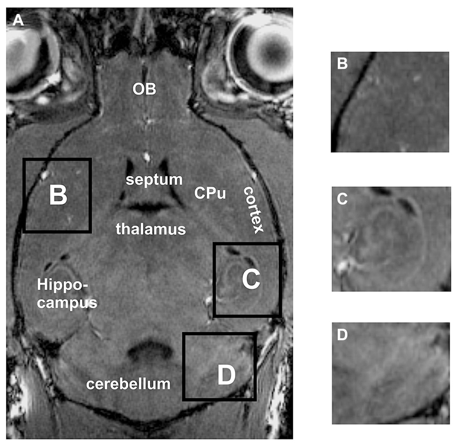
FIGURE 1. By using in vivo tissue, the brain and the surrounding tissue are clearly visible (A). However, the boundaries between the cortex and the CPu are difficult to detect (A,B). Neither the hippocampal fields CA1, CA3 nor the dentate gyrus can clearly be distinguished (C). Within the cerebellum (D) the different layers cannot be differentiated. Inserts B,C,D represent magnifications of areas shown in A. CPu, caudate putamen; OB, olfactory bulb.

Post-mortem MRI at 7 Tesla allows visualization of the murine brain in greater detail. Thus, using maximum intensity projection of the entire scan, the brain surface along with the blood vessels was clearly visible (Figure 2A). Without use of any fixation or contrast enhancing agents, not only the brain could be distinguished from the surrounding tissue, but also substructures could be differentiated (Figures 2B,C). Thus, not only cortical areas could be distinguished from, e.g., the CPu, but also the external capsule could be recognized, as well as different parts of the olfactory bulb, corresponding to different layers of the olfactory bulb (Figure 2B). For the cerebellum the white matter tracts and the granular and molecular layer could be distinguished (Figures 2D,E) but not the cerebellar Purkinje-cell layer.

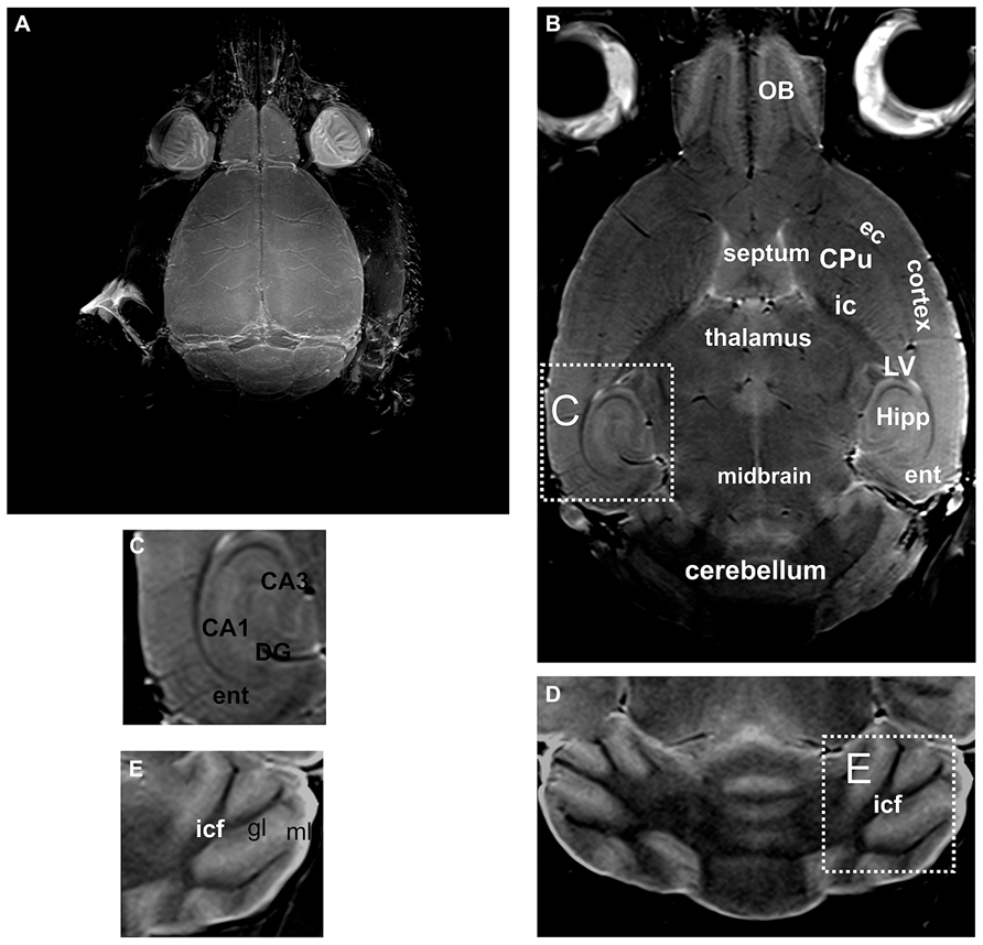
FIGURE 2. By using unfixed post-mortem tissue, the brain and the blood vessels located on the brain surface are clearly visible in an intensity projection of the 3D scan (A). A representative slice through a 3D volume of un-fixed post-mortem head of a mouse is shown in (B). A higher magnification of the hippocampal formation is shown in (C). Likewise in the cerebellum (D) the white matter tracts and the gray matter can be distinguished. However, the Purkinje cell layer, which is composed of a single layer of relatively large neurons, cannot be detected (a higher magnification of this area is shown in E). CA1, CA3, hippocampal area; CPu, caudate putamen; DG, dentate gyrus; ec, external capsule; ent, entorhinal cortex; gl, granular layer of the cerebellum; Hipp, hippocampus; ic, internal capsule; icf, intercrural fibers; LV, lateral ventricle; ml, molecular layer of the cerebellum; OB, olfactory bulb.

Concerning the fixed extracted brains, the structure was less well preserved (Figure 3). This confirms that fixation produces loss in quality (see Introduction section). In addition, brains were in an advanced state of decomposition due to the long delay between euthanasia and extraction. This resulted in partial tissue damage during the extraction procedure. In our approach, the brains were deformed by the flask used for their storage (see Figure 3). This latter problem could be overcome by using a different mode of storage.

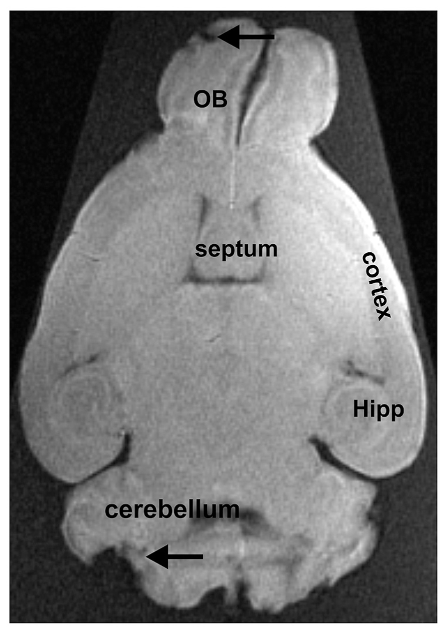
FIGURE 3. Extracted brain tissue that was fixed for several days. The olfactory bulbs (OB), the cortex, the hippocampus (Hipp), and the cerebellum can easily be distinguished from adjacent brain regions. Due to the removal of the brain from the surrounding tissue, some damage can be noted, as e.g., in the cerebellum or the OB (indicated by arrows).

No statistical significant shrinkage for the post-mortem brains was observed as compared to the in vivo brains (Figure 4). Short fixation did also not result in statistical significant shrinkage, but induced a larger variance (Figure 4). In contrast, long-term fixation was found to induce a significant shrinkage of the cortical thickness (Figure 4).

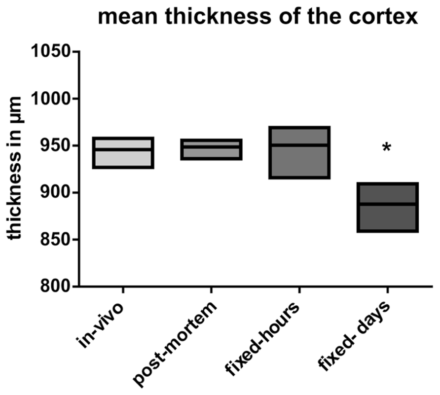
FIGURE 4. Analysis of the mean thickness of the cortex. Data are presented as mean ± min to max (*p ≤ 0.05; ANOVA; Tukey’s post hoc test). In vivo: data from the in vivo scanning procedure; post-mortem: data obtained by using post-mortem brains; fixed-hours: data obtained by using extracted brains that were fixed for some hours; fixed-days: data obtained from extracted brains that were fixed for several days.

Preprocessing and Automatic Segmentation

An IIC was necessary to achieve a good segmentation of the in vivo scans, which included all brain regions (Figures 5A,C,G). Parts of the cerebellum where missing in the segmentation if IIC was not applied. The post-mortem scans did not need any preprocessing to achieve an excellent segmentation (Figures 5B,D,H). In vivo and post-mortem segmentations both contained non-brain tissue in the gray matter segmentation, visible in Figures 5A–D as white stripes encompassing the outer limit of the gray matter. Brain extraction preceding segmentation decreased the amount of non-brain tissue in the segmentation. Applying IIC or modifying SPMMouse parameters also changed the tissue volumes. However, volumes of in vivo and post-mortem scans did not converge against identical values regardless of the fine tuning procedures. Therefore, the minimum number of processing steps preceding segmentation and standard SPMMouse parameters were chosen.

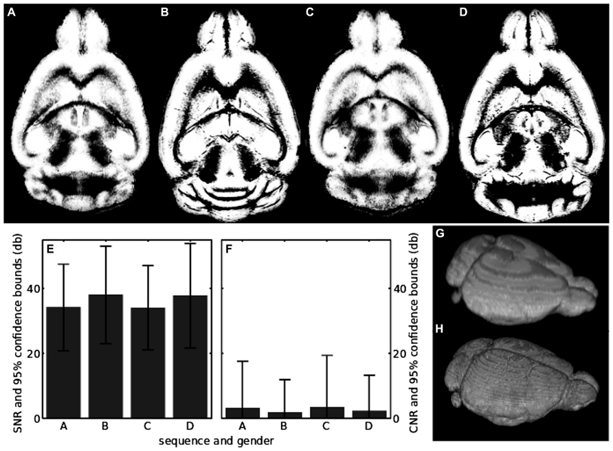
FIGURE 5. (A) Center slice in the segmentation of the in vivo sequence for the female mouse; (B) same as in A, but for the post-mortem scan; (C) segmentation of the in vivo sequence for the male mouse; (D) the same as in C, but for the post-mortem scan; (E) SNR of raw unsegmented in vivo and post-mortem scans. The labels on the horizontal axis show which sequence and mouse has been analyzed and correspond to the upper row of the figure; (F) the same as in E, but for the CNR; (G) volume visualization of the in vivo segmentation result shown in A; (H) volume visualization of the post-mortem segmentation result shown in B.

This was done to minimize errors due to the processing and to achieve maximum comparability to literature values. In case of in vivo scans, the gray matter volumes for the female and male mouse differed by less than 2% (Table 1), while the post-mortem scans differed by less than 4% (Table 1). The maximum difference between in vivo and post-mortem scan gray matter volume was 8% (see Table 1).

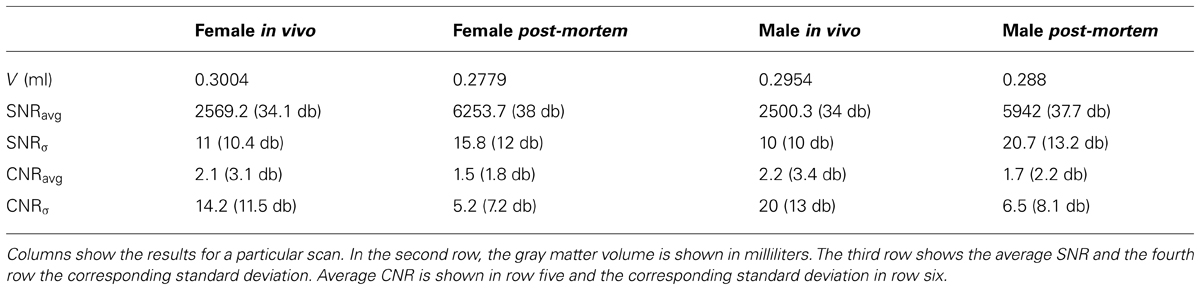
TABLE 1. Quantitative results from post-processing.

The SNRs of all scans together with their standard deviations are shown in Table 1 and depicted in Figure 5E. In vivo scans exhibited an SNR_avg > 34 db and post-mortem scans had an SNR_avg > 37 db. All scans had a lower limit of the SNR_avg > 20 db if the 95% confidence bound was taken into account. Thus, the brain signal of the image was at least 100 times larger than the noise. The corresponding results for the CNR of all scans and its standard deviation are also shown in Table 1 and depicted in Figure 5F. In vivo scans exhibited a CNR_avg > 2.1 db and post-mortem scans had a CNR_avg > 1.5 db. Thus, gray and white matter contrasts differ on average about 50% in their contrast values. Notably, CNR_avg of in vivo scans was slightly larger than of post-mortem scans. The opposite was found for the standard deviations of the CNRs, which was probably due to a higher effect of intensity inhomogeneities in the in vivo scans. CNR_σ was larger than CNR_avg by at least a factor 6 for the in vivo scans, while it was at least a factor of 3 for the post-mortem scans.

Discussion

We demonstrate that the use of non-fixed post-mortem tissue is well-suited as a quick and sensitive method for high-resolution MRI. Several technical difficulties found previously at 7 Tesla MRI (Beuf et al., 2006) were dissolved, leading to high-throughput capabilities. Damage due to the removal of the brains and time-consuming tissue processing, possibly leading to severe shrinkage or other fixation artifacts, are avoided. Compared to the in vivo situation, artifacts due to respiration and cardiac activity are absent and longer scan times are possible. This allows applying T2-weighted sequences with high spatial resolution and contrast, as compared to fast T1-weighted sequences applied in vivo.

The qualitative inspection of in vivo, post-mortem and ex situ scans confirmed the results found in the literature concerning in vivo and ex situ scans. An identification of substructures in in vivo scans was difficult due to the low quality of the scans, but could be achieved at various positions for the cortex. In ex situ scans fixation artifacts, deformations and damages affected the scans severely and complicated the reliable identification of brain substructures. These artifacts may occur during the formalin fixation process (Benveniste and Blackband, 2006).

The thickness analysis of the cortical layer indicated that significant shrinkage was found for brains fixated for days, while no shrinkage was found if brains were fixated for hours only or without fixation. Along this line, in a recent MRI study, using human post-mortem brain that have been fixed with formalin, it has been shown that fixation resulted after several days in substantial tissue shrinkage and local deformations (Schulz et al., 2011). In histology, the impact of different fixatives on tissue shrinkage is well known (Stickland, 1975) and recently the impact of formaldehyde fixation on distortion of brain tissue has been re-examined in detail (Weisbecker, 2012). Since shrinkage of the tissue was found to have an impact on stereological estimates, a volumetric shrinkage factor has been introduced (Jinno et al., 1999). Paraformaldehyde fixation, sectioning and staining of mouse brain sections, and subsequent embedding can produce a volumetric shrinkage factor of about 0.6 (von Bohlen und Halbach and Unsicker, 2002). Thus, post-processing of the tissue, like the use of contrast enhancing substances on formaldehyde fixated brains for MRI scans, may let to further tissue distortion. Techniques developed for shrinkage correction in histological specimens are unfortunately not applicable for MR imaging analysis. However, algorithms compensating for volumetric shrinkage and tissue distortion due to fixation (Schulz et al., 2011) are not necessary if non-fixated post-mortem brains are investigated in situ.

Overall, the post-mortem scans allowed for a more distinct identification of substructures than the in vivo scans, and exhibited minimal influence of artifacts. This was also confirmed for the entire gray matter in the post-mortem scan using IIC and SPMMouse brain segmentation techniques. The maximum difference between in vivo and post-mortem scan gray matter volume was 8%, which confirms the result for cortical thickness depicted in Figure 4. Only one ex situ brain dataset allowed for an automatized segmentation. This was due to alterations in the brain caused by fixation, extraction and/or deformation during storage. Since the ex situ brains have to be investigated in carriers, a positioning of surface MRI-coils near the brain is hampered, too. This might also decrease MRI-signal intensity, which might well result in problems in segmentation (Ashburner and Friston, 2005).

The contrast-to-noise ratio (CNR) is highly important for the differentiation between tissues in MRI scans. SNR of the scans is excellent at 7T and shows relevant improvement if compared to MRI at lower field strengths (Natt et al., 2002). However, the CNR is rather small and changes considerably between measurements. On average gray and white matter contrasts differ by 50% in their contrast values in the in vivo and post-mortem scans. Since the quality of the automatic segmentation will depend on CNR, optimization of MRI sequences at 7 Tesla should aim on improving the CNR. This could be achieved in the post-processing using an IIC. Further optimization of sequence parameters might result in improved CNR (DiFrancesco et al., 2008) and minimized intensity inhomogeneities (Tannus and Garwood, 1997).

Cleary and colleagues described that the usage of contrast enhancing agent gadolinium on fixated brains in a 9.4 Tesla scanner allowed for visualization of the Purkinje cell layer of the cerebellum (Cleary et al., 2011). In our approach, the resolution was not high enough to distinguish single Purkinje cells or other single neurons; a problem that might be overcome by using a 9.4 T scanner. The use of the post-mortem MRI technique is, however, much faster and may therefore be a valuable method for anatomical phenotyping of transgenic mice. In addition, it enables an increase in the throughput for MRI phenotyping of large numbers of rodents, allowing to determine very quickly small structural alterations in the murine brain at a reasonably high resolution even with 7 Tesla field strength. Furthermore, an increase in scanning times will no longer represent a limiting factor for obtaining higher resolutions.

Conflict of Interest Statement

The authors declare that the research was conducted in the absence of any commercial or financial relationships that could be construed as a potential conflict of interest.

Acknowledgments

Stefan Hadlich is acknowledged for his excellent service and support of the MRI scanner examinations and Dr. Katharina Kindermann for her veterinary administration during the examinations.

References

Ashburner, J., and Friston, K. J. (2005). Unified segmentation. Neuroimage 26, 839–851. doi: 10.1016/j.neuroimage.2005.02.018
Benveniste, H., and Blackband, S. (2002). MR microscopy and high resolution small animal MRI: applications in neuroscience research. Prog. Neurobiol. 67, 393–420. doi: 10.1016/S0301-0082(02)00020-5
Benveniste, H., and Blackband, S. J. (2006). Translational neuroscience and magnetic-resonance microscopy. Lancet Neurol. 5, 536–544. doi: 10.1016/s1474-4422(06)70472-0
Benveniste, H., Kim, K., Zhang, L., and Johnson, G. A. (2000). Magnetic resonance microscopy of the C57BL mouse brain. Neuroimage 11, 601–611. doi: 10.1006/nimg.2000.0567
Beuf, O., Jaillon, F., and Saint-Jalmes, H. (2006). Small-animal MRI: signal-to-noise ratio comparison at 7 and 1.5 T with multiple-animal acquisition strategies. MAGMA 19, 202–208. doi: 10.1007/s10334-006-0048-9
Buxton, R. B. (2009). Introduction to Functional Magnetic Resonance Imaging. Cambridge University Press. doi: 10.1017/CBO9780511605505
Cahill, L. S., Laliberte, C. L., Ellegood, J., Spring, S., Gleave, J. A., Eede, M. C., et al. (2012). Preparation of fixed mouse brains for MRI. Neuroimage 60, 933–939. doi: 10.1016/j.neuroimage.2012.01.100
Chou, N., Wu, J., Bai Bingren, J., Qiu, A., and Chuang, K. H. (2011). Robust automatic rodent brain extraction using 3-D pulse-coupled neural networks (PCNN). IEEE Trans. Image Process. 20, 2554–2564. doi: 10.1109/tip.2011.2126587
Cleary, J. O., Wiseman, F. K., Norris, F. C., Price, A. N., Choy, M., Tybulewicz, V. L., et al. (2011). Structural correlates of active-staining following magnetic resonance microscopy in the mouse brain. Neuroimage 56, 974–983. doi: 10.1016/j.neuroimage.2011.01.082
DiFrancesco, M. W., Rasmussen, J. M., Yuan, W., Pratt, R., Dunn, S., Dardzinski, B. J., et al. (2008). Comparison of SNR and CNR for in vivo mouse brain imaging at 3 and 7 T using well matched scanner configurations. Med. Phys. 35, 3972–3978. doi: 10.1118/1.2968092
Huang, S., Liu, C., Dai, G., Kim, Y. R., and Rosen, B. R. (2009). Manipulation of tissue contrast using contrast agents for enhanced MR microscopy in ex vivo mouse brain. Neuroimage 46, 589–599. doi: 10.1016/j.neuroimage.2009.02.027
Jinno, S., Aika, Y., Fukuda, T., and Kosaka, T. (1999). Quantitative analysis of neuronal nitric oxide synthase-immunoreactive neurons in the mouse hippocampus with optical disector. J. Comp. Neurol. 410, 398–412. doi: 10.1002/(SICI)1096-9861(19990802)410:3<398::AID-CNE4>3.0.CO;2-9
Johnson, G. A., Benveniste, H., Black, R. D., Hedlund, L. W., Maronpot, R. R., and Smith, B. R. (1993). Histology by magnetic resonance microscopy. Magn. Reson. Q. 9, 1–30.
Kim, S., Pickup, S., Hsu, O., and Poptani, H. (2009). Enhanced delineation of white matter structures of the fixed mouse brain using Gd-DTPA in microscopic MRI. NMR Biomed. 22, 303–309. doi: 10.1002/nbm.1324
Ma, Y., Hof, P. R., Grant, S. C., Blackband, S. J., Bennett, R., Slatest, L., et al. (2005). A three-dimensional digital atlas database of the adult C57BL/6J mouse brain by magnetic resonance microscopy. Neuroscience 135, 1203–1215. doi: 10.1016/j.neuroscience.2005.07.014
Natt, O., Watanabe, T., Boretius, S., Radulovic, J., Frahm, J., and Michaelis, T. (2002). High-resolution 3D MRI of mouse brain reveals small cerebral structures in vivo. J. Neurosci. Methods 120, 203–209. doi: 10.1016/S0165-0270(02)00211-X
Paxinos, G., and Franklin, K. B. J. (2001). The Mouse Brain in Stereotaxic Coordinates. San Diego: Academic press.
Sawiak, S. J., Wood, N. I., Williams, G. B., Morton, A. J., and Carpenter, T. A. (2009). Voxel-based morphometry in the R6/2 transgenic mouse reveals differences between genotypes not seen with manual 2D morphometry. Neurobiol. Dis. 33, 20–27. doi: 10.1016/j.nbd.2008.09.016
Schulz, G., Crooijmans, H. J., Germann, M., Scheffler, K., Muller-Gerbl, M., and Muller, B. (2011). Three-dimensional strain fields in human brain resulting from formalin fixation. J. Neurosci. Methods 202, 17–27. doi: 10.1016/j.jneumeth.2011.08.031
Sled, J. G., Zijdenbos, A. P., and Evans, A. C. (1998). A nonparametric method for automatic correction of intensity nonuniformity in MRI data. IEEE Trans. Med. Imaging 17, 87–97. doi: 10.1109/42.668698
Stickland, N. C. (1975). A detailed analysis of the effects of various fixatives on animal tissue with particular reference to muscle tissue. Stain Technol. 50, 255–264. doi: 10.3109/10520297509117068
Szczesny, G., Veihelmann, A., Massberg, S., Nolte, D., and Messmer, K. (2004). Long-term anaesthesia using inhalatory isoflurane in different strains of mice-the haemodynamic effects. Lab. Anim. 38, 64–69. doi: 10.1258/00236770460734416
Tannus, A., and Garwood, M. (1997). Adiabatic pulses. NMR Biomed. 10, 423–434. doi: 10.1002/(SICI)1099-1492(199712)10:8<423::AID-NBM488>3.0.CO;2-X
von Bohlen und Halbach, O., Minichiello, L., and Unsicker, K. (2008). TrkB but not trkC receptors are necessary for postnatal maintenance of hippocampal spines. Neurobiol. Aging 29, 1247–1255. doi: 10.1016/j.neurobiolaging.2007.02.028
von Bohlen und Halbach, O., and Unsicker, K. (2002). Morphological alterations in the amygdala and hippocampus of mice during ageing. Eur. J. Neurosci. 16, 2434–2440. doi: 10.1046/j.1460-9568.2002.02405.x
Weisbecker, V. (2012). Distortion in formalin-fixed brains: using geometric morphometrics to quantify the worst-case scenario in mice. Brain Struct. Funct. 217, 677–685. doi: 10.1007/s00429-011-0366-1
Keywords: spatial resolution, animal scanner, in vivo, MRI, segmentation, post-mortem, signal-to-noise ratio, contrast-to-noise ratio
Citation: von Bohlen und Halbach O, Lotze M and Pfannmöller JP (2014) Post-mortem magnetic resonance microscopy (MRM) of the murine brain at 7 Tesla results in a gain of resolution as compared to in vivo MRM. Front. Neuroanat. 8:47. doi: 10.3389/fnana.2014.00047
Received: 28 March 2014; Accepted: 28 May 2014;
Published online: 13 June 2014.
Edited by:
George Paxinos, University of New South Wales, AustraliaReviewed by:
Marten P. Smidt, University of Amsterdam, NetherlandsDean Dessem, University of Maryland, USA
Copyright © 2014 von Bohlen und Halbach, Lotze and Pfannmöller. This is an open-access article distributed under the terms of the Creative Commons Attribution License (CC BY). The use, distribution or reproduction in other forums is permitted, provided the original author(s) or licensor are credited and that the original publication in this journal is cited, in accordance with accepted academic practice. No use, distribution or reproduction is permitted which does not comply with these terms.
*Correspondence: Oliver von Bohlen und Halbach, Institut für Anatomie und Zellbiologie, Universitätsmedizin Greifswald, Friedrich Loeffler Street 23c, 17487 Greifswald, Germany e-mail: oliver.vonbohlen@uni-greifswald.de