Learning Corrections for Hyperelastic Models From Data
 David González1
  Elías Cueto
- 1Aragon Institute of Engineering Research, Universidad de Zaragoza, Zaragoza, Spain
- 2ESI Group Chair and PIMM Lab, ENSAM ParisTech, Paris, France
Unveiling physical laws from data is seen as the ultimate sign of human intelligence. While there is a growing interest in this sense around the machine learning community, some recent works have attempted to simply substitute physical laws by data. We believe that getting rid of centuries of scientific knowledge is simply nonsense. There are models whose validity and usefulness is out of any doubt, so try to substitute them by data seems to be a waste of knowledge. While it is true that fitting well-known physical laws to experimental data is sometimes a painful process, a good theory continues to be practical and provide useful insights to interpret the phenomena taking place. That is why we present here a method to construct, based on data, automatic corrections to existing models. Emphasis is put in the correct thermodynamic character of these corrections, so as to avoid violations of first principles such as the laws of thermodynamics. These corrections are sought under the umbrella of the GENERIC framework (Grmela and Oettinger, 1997), a generalization of Hamiltonian mechanics to non-equilibrium thermodynamics. This framework ensures the satisfaction of the first and second laws of thermodynamics, while providing a very appealing context for the proposed automated correction of existing laws. In this work we focus on solid mechanics, particularly large strain (visco-)hyperelasticity.
1. Introduction
In a very recent paper about how construct machines that could eventually learn and think like humans, Lake et al. (2017) state that “machines should build casual models of the world that support explanations and understanding, rather than merely solving pattern recognition problems” and that “model building is the hallmark of human-level learning, or explaining observed data through the construction of causal models of the world”. Indeed, machine learning of physical laws could be seen as the ultimate form of machine intelligence, and this should be done, of course, from data.
There is a very active field of research around this way of reasoning. For instance, in Brunton et al. (2016) a method is presented that operates on a bag of terms like sines, cosines, exponentials, etc., so as to find an expression that is sparse (i.e., it incorporates few of theses terms) while still explaining the experimental data. Similar approaches include techniques to find reduced-order operators from data (Peherstorfer and Willcox, 2015, 2016) or the possibility to construct physics-informed machine learning (Raissi et al., 2017a,b; Swischuk et al., 2018).
In the field of computational materials science, this approach seems to begin by the works of Kirchdoerfer and Ortiz (2016, 2017a). In it, and the subsequent works, they present a method in which the constitutive equation is substituted by experimental data, that could be possibly noisy (Kirchdoerfer and Ortiz, 2017b; Ayensa-Jiménez et al., 2018). In them, it is recognized that some equations (notably, equilibrium, compatibility) are of a higher epistemic nature, while constitutive equations—that are often phenomenological and, therefore, of lower epistemic value—could easily be replaced by data (Latorre and Montáns, 2014). The criterion is to establish a distance measure that indicates the closest experimental datum to be employed every time the constitutive law is called at the finite element integration point level.
In some of our previous works, this approach is further generalized by defining the concept of constitutive manifold, a low-dimensional embedding for the stress-strain pairs (see Lopez et al., 2018). Thus, by alternating between stress-strain pairs that satisfy either equilibrium or the constitutive equation, the solution that satisfies the three families of equations is found, regardless of the non-linearity of the behavior. Several methods have been studied for the construction of this constitutive manifold (Ibañez et al., 2017).
Another inherent difficulty in trying to machine learning models is that of the adequate level of description. Every physical phenomenon can be described at different levels of detail. In the case of fluid mechanics, for instance, these levels range from molecular dynamics to thermodynamics—in descending order of detail—. In between, different theories have been developed that take care of different descriptors of the phenomenon taking place: from the Liouville description to the Fokker-Planck equation, hydrodynamics, …to name but a few of the different possibilities (Español, 2004). Thus, there should be a compromise between detail in the description and the resulting computational tractability of the approach. This is something very difficult to discern for an artificial intelligence.
The risk of employing an approach based upon pure data regression is to violate—due to the inherent noise in data, for instance—some basic principles such as the laws of thermodynamics: conservation of energy, positive dissipation of entropy. Trying to avoid these possible inconsistencies, in González et al. (2018) we developed a data-driven method that operates under the framework of the GENERIC formalism (Grmela and Oettinger, 1997; Öttinger, 2005). The General Equation for Non-Equilibrium Reversible-Irreversible Coupling (GENERIC) constitutes a generalization of the Hamiltonian mechanics. Therefore, under the GENERIC umbrella, the equations satisfy basic thermodynamic principles by construction.
Thus, the problem translates to finding—by means of data—the right expression of the particular GENERIC formalism for the system at hand (or its finite element approximation, if we work in a purely numerical framework). The resulting approximation is thermodynamically sound and very appealing from the numerical point of view. The stability of the GENERIC approach and its thermodynamic consistency—in particular, the conservation of symmetries in the formulation—has been thoroughly investigated in previous works, whose lecture is greatly recommended (Romero, 2009, 2010).
However, even if the usual parameter fitting procedure from experimental data is often painful and, notably, gives poor fitting of the results in many occasions, we believe that well-known constitutive equations should not be discarded, thus waiting centuries of scientific discovery. Instead, we believe that it is interesting to simply correct those models that sometimes do not fit perfectly the results—sometimes locally, in a delimited region of the phase space—. This is the approach followed in Ibañez et al. (2018), where corrections are developed to yield criteria so as to render them compliant (to a specified tolerance level) with the available experimental results. A similar approach has been pursued recently in Lam et al. (2017) for a study on the interaction of aircraft wings. In these approaches, the chosen level of description is defined by the (poor) model, so, in principle, no further decision needs to be taken, as will be discussed later on.
The GENERIC formalism is valid for all levels of description, and could also help in deriving corrections from data that still maintain the thermodynamic properties of the resulting model. Hyperelastic models fall within Hamiltonian mechanics—i.e., they represent a purely conservative material—. However, rubbers or foams usually present some degree of viscoelasticity, for instance. In this framework, Hamiltonian mechanics will no longer be the right formalism to develop their constitutive equations. GENERIC should be preferred instead.
In this paper we study how to learn these corrections from data. First, in Section 2 we review the basics of the GENERIC formalism, with an emphasis on hyperelastic and visco-hyperelastic materials. In Section 3 we explain how to employ GENERIC to develop corrections to existing models from data, while in Section 4 we introduce, by means of an academic example in finite dimensions, the basic ingredients of our approach. This will be further detailed for visco-hyperelastic materials in Section 5. The paper ends with a discussion on the just developed techniques and the future lineas of research in Section 6.
2. A Review of the Generic Formalism
2.1. The Basics
The GENERIC formalism was introduced by Grmela and Oettinger (1997) in a seminal paper in an attempt to give a common structure for non-Newtonian fluid models. The establishment of such a model in the GENERIC framework starts by selecting appropriate state variables. This is not straightforward in a general case in which we have no prior information about the precise behavior of the system at hand. However, for most systems—and specially when we start from known models, as it is the case in this work—simple rules exist for the selection of such variables (Öttinger, 2005). Selecting mutually dependent variables does not constitute a problem, in fact, as most of the literature on GENERIC demonstrates. Let us call these variables , , and emphasize their obvious time dependency in the interval . represents the space in which these variables live, which depends obviously on the particular system under scrutiny. The final objective of the GENERIC model is to establish an expression for the time evolution of these variables, .
The GENERIC equation takes, under these assumptions, the form
The first sum on the right-hand side term represent the Hamiltonian, or conservative, part of the behavior of the system. In it, the term L(zt) is the so-called Poisson matrix. The second sum is responsible for the dissipative behavior of the system, with M(zt) the so-called friction matrix. Here, E(zt) represents the total energy of the system, while S(zt) represents its entropy.
For Equation (1) to give a valid description of any physical system, it must be supplemented with the so-called degeneracy conditions:
Enforcing these conditions leads to the necessity of L(z) to be skew-symmetric and a M to be symmetric, positive semi-definite. If these conditions are met, then, it holds,
which is, in fact, the equation of conservation of energy for the system. Additionally, these conditions ensure the satisfaction of
or, equivalently, the fulfillment of the second principle of thermodynamics.
Noteworthy, Equation (1) constitutes the most general framework to develop a valid constitutive equation in the light of the principles of thermodynamics. A valid constitutive model must satisfy the GENERIC equation, and any possible correction to it should not deviate the result from this framework. For a thorough description of a long list of models under the GENERIC formalism, the interested reader can consult Öttinger (2012). To exemplify the just introduced concepts, consider the simplest case of a conservative mechanical system whose time evolution can be expressed, in the Hamiltonian framework, by resorting to a description of the type , where qt represents the position and pt the momentum. In that situation, the system is purely Hamiltonian and
with no entropy evolution, i.e., M = 0. In this simple situation, L(z) turns out to be the canonical symplectic matrix and the GENERIC description of the system reduces to that of a Hamiltonian system.
2.2. Hyperelasticity Under the Prism of GENERIC
It is important to highlight the fact that, for hyperelastic materials, the expression
represents the usual hyperelastic problem under the Hamiltonian formalism (Romero, 2013). Indeed, if we choose z(x, t) = [x(X, t), p(X, t)]⊤, where x = ϕ(X)—the deformed configuration of the solid—and p represents the material momentum density, then,
The total energy of an elastic body Ω can be decomposed as
i.e., the sum of elastic and kinetic energies. Here, we assume a strain energy density potential w of the form
where C represents the right Cauchy-Green deformation tensor. While, in general, the strain energy density for an isotropic case would be of the form w = w(X, C, S), in the context of isotropic hyperelasticity—a purely Hamiltonian case—, this dependence is often simply w = w(C). In turn, the kinetic energy will be
In this framework, it is clear that
where P and S represent, respectively, the first and second Piola-Kirchhoff stress tensors and F is the deformation gradient. Given that
with V the material velocity and ρ0 the density in the reference configuration so that, finally,
This implies that
which is fully compliant with the GENERIC framework, see Equation (1). This model is readily seen as equivalent to
which correspond to the definition of the material momentum density and the equilibrium equation, respectively.
Under this rationale, the possible viscous effects in the material would be described by the second sum in Equation (1).
REMARK. We have stated that, under the GENERIC formalism, an isotropic Hamiltonian or conservative hyperelastic model can be written in the form w = w(C) and therefore will not depend on S. This discussion is strongly related with that of the adequate level of description of the model. In fact, many hyperelastic models exist that depend on different parameters, that can influence its viscous behavior, for instance, see Mihai and Goriely (2017).
Indeed, by introducing a new potential (entropy) in the formulation, what we are doing is to introduce ignorance on these details, while still taking into account their influence on the results. It is the same process we face if we are not interested in tracking every molecule of a gas in a container but prefer instead a description based on macro-scale magnitudes such as pressure, volume, and temperature. The process of coarse-graining the description in a non-equilibrium setting makes it necessary to introduce a new potential that accounts for the neglected information: entropy (Español, 2004; Pavelka et al., 2018). Thus, in the correction procedure that we are about to introduce, there will be no need to add new variables to the model, but an adequate entropy potential to the formulation.
The problem of constructing a valid constitutive model under the GENERIC point of view is therefore reduced to that of finding the particular structure of the terms L(z), E(z), M(z), and S(z). The classical approach is to do it analytically, as in Romero (2009, 2010), for instance, or Vázquez-Quesada et al. (2009) and Español (2004), to name but a few of the examples in the literature. A different approach is to find the structure of these terms numerically, from data. This will be done possibly with the help of manifold learning techniques such as LLE (Roweis and Saul, 2000) or isomap (Tenenbaum et al., 2000), among others. It is the approach followed by the authors in González et al. (2018) and, in some sense, it is also the approach followed by Millán and Arroyo (2013) without even knowing the structure of GENERIC. This approach is also somehow related to the use of compositional rules to construct models (Grosse et al., 2012). This last reference shares with the approach herein the need of identifying the structure of several matrices that are then used to develop models—in that case, of phenomena that do not even obey the laws of physics, such as voting tendencies, for instance.
3. Correcting Models in a Generic Framework
In this work we do not pursue to unveil models by means of GENERIC and experimental data. As explained in the introduction, we believe that is simply nonsense to discard models that have demonstrated to be useful for decades. In the case of hyperelasticity, these include, among a wide list of references, the works of Treloar (1975), Ogden (1984) or Holzapfel and Gasser (2000). These models, as analyzed before, already had a GENERIC structure.
Purely hyperelastic materials are strictly conservative. However, soft living matter, for instance, that is often modeled under the hyperelastic theory, present some non-negligible viscous effects (Peña et al., 2011; Garćıa et al., 2012). In that case, in the light of the GENERIC formalism, it is necessary to complement the model with a dissipative part, i.e., to determine the precise form of M(z) and S(z).
What we will do in this work, in fact, is to assume that an inexact model exists, so that a correction is needed,
where “corr”, “exp” and “mod” stand, respectively, for correction, experimental and model. We will develop a correction in the GENERIC framework so as to guarantee that the corrected model for the experimental results will also have a GENERIC structure. To this end, we cast the correction in the form
We do not consider a correction for L nor M, since, in the light of the previous remark, L is assumed to be identical to that of the model (we consider the same state variables). Since the correction of the model could have an important influence on the form of M—recall again the remark in the previous section, we attribute to S the possible presence of fine-grained state variables that are not considered in the Hamiltonian part of the model—, we discard any possible M coming from the inexact model and instead re-compute it from scratch. With these assumptions, the resulting model that fits with the experimental results will have the form
so that, finally,
which proves that the corrected model for zexp possesses a GENERIC structure with a correction in the Hamiltonian term.
Consider that a set of nmeas experimental measurements is available. The predictions of the inexact model are then subtracted from the experimental results. The final objective will be therefore to obtain a discrete approximation
to the GENERIC structure of the discrepancy between data and experiments, by identifying DE(z), and possibly also M(z) and DS(z). DE and DS represent the discrete gradients (in a finite element sense).
Therefore, the proposed algorithm will consist in solving the following (possibly constrained by the degeneracy conditions) minimization problem within a time interval :
with zmeas ⊆ Z, a subset of the total available experimental results. See the discussion in González et al. (2018) about how to determine the right size of the sample set, the possibility of employing monolithic or staggered strategies, etc.
In the next Section this procedure is exemplified with the help of an academic example in finite dimensions.
4. An Introductory Example
We first consider an example analyzed in Romero (2009) and then again in González et al. (2018). The system is a double pendulum, which is connected by thermoelastic springs. It comprises two masses m1 and m2 connected by springs of internal energy e1 and e2. They oscillate around a fixed point, see (Figure 1). We employ the classical notation of Hamiltonian mechanics where qi, pi, i = 1, 2 represent position and momenta, respectively. For the springs, their respective entropies are sj, and the longitudes at rest will be denoted by , j = a, b.
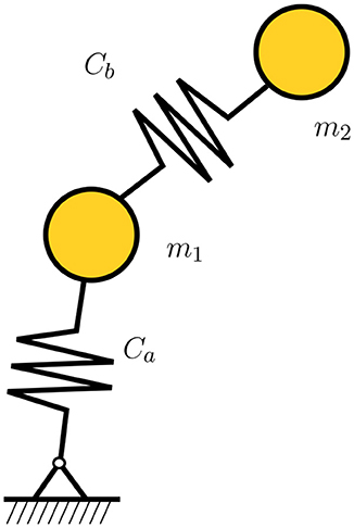
Figure 1. Double thermal pendulum.
The set of state variables for this double pendulum will be therefore
The GENERIC structure for this problem needs to consider the internal energy of the system. Again, the internal energy is composed by the kinetic energy of the masses and the potential energy in the springs, i.e.,
with
The temperature in the springs, θj, is assumed to be originated by the Joule effect,
The conductivity in the springs will be denoted by κ. Under this rationale, the resulting equations for the double pendulum will be
with i = 1, 2, j = a, b, k≠j. Therefore, the gradients of the GENERIC formalism will look
with fj, nj, j = a, b, the forces in the springs and their respective unit vector along their direction.
Poisson and friction matrices will result in this case,
However, we will assume that this description of the system is not available—will be used as a ground truth to determine errors—and that the system is thought to be purely Hamiltonian.
In this scenario, the goal of our method will be that of unveiling the dissipative part of the model so as to correct the pure Hamiltonian behavior of the assumed model. In other words, the system will be considered as modeled by
with L as in Equation (7) and ∇E as defined in Equation (6a). Results of the ground truth, the assumed (purely Hamiltonian) model and the found corrected model are shown in Figure 2.
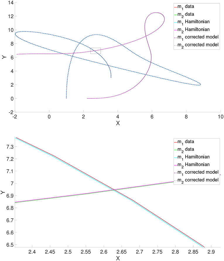
Figure 2. Results for the thermal pendulum problem. Results are shown (see the detail in the small window in the bottom figure) for the ground truth (pseudo-experimental data), the uncorrected (purely Hamiltonian) assumed model and the corrected one.
The mean squared error of the assumed model with respect to the pseudo-experimental data was initially 0.1732%. Note the little influence of the Joule effect on the results. However, after a correction is found and the dissipative character of the model is taken into account, this error is decreased up to 0.0125%, i.e., one order of magnitude.
5. Corrections to Hyperelastic Models
In order to show the full capabilities of the proposed method, we consider now an example of a visco-hyperelastic material whose precise constitutive model is to be corrected from experimental data.
5.1. Ground Truth. Pseudo-Experimental Data
The pseudo-experimental data is obtained by finite element simulation of a visco-hyperelastic Mooney-Rivlin material in which
with and , and where the invariants of the right Cauchy-Green tensor C are defined as , and , respectively. J represents, as usual, the determinant of the gradient of deformation tensor. In this case, C1 = 27.56 MPa, C2 = 6.89 MPa and D1 = 0.0029 MPa.
To model the viscoelastic behavior of this rubberlike material, it is assumed that the material's shear modulus G and bulk modulus K evolve in time. This evolution is modeled by means of a Prony series in terms of the instantaneous moduli,
with and . The relaxation times take the values τi = [0.1, 0.2] seconds, respectively. With these values, the initial instantaneous Young's modulus takes the value E = 206.7 MPa, with Poisson's ratio ν = 0.45.
Data was generated after a total of 557 different loading processes to the same specimen. It was subjected to a load history of different amplitudes. In every case, a first plane stress state (σx, σy, τxy)—values are not correlated—is applied during a short impulse of 0.021 seconds, then maintained at constant value for one more second, allowing the material to creep. This is followed by a second loading process of 0.021 seconds at a different (σx, σy, τxy) value, followed by a final plateau of one more second. For each one of the 557 different experiments these two stress states were different. These results are stored in the form of 557 different Z vectors, thus representing a trajectory in time.
5.2. Modeling the Results With a Purely Hyperelastic Model
After the generation of the pseudo-experimental data, we tried to reproduce these results with a deliberately wrong model: the material was assumed to be modeled by a Mooney-Rivlin model with no viscous response (and thus purely Hamiltonian or conservative). The comparison of the experimental results and the predictions given by this (poor) model are shown in Figure 3.
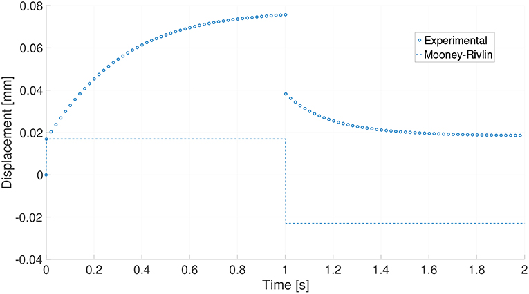
Figure 3. Loading process for one particular experiment. Pseudo-experimental response and prediction made by the standard (non-viscous) Mooney-Rivlin material.
It seems obvious that a classical Mooney-Rivlin model can not reproduce the viscous behavior of the reference material. In the next section a correction to this model is developed based on the available data and the procedure introduced in Section 3.
5.3. Correction of the Dissipative Part of the Model
Knowing in advance that the pseudo-experimental results come from a viscous modification to a Mooney-Rivlin model, a first attempt is made of finding a correction by incorporating a dissipative part in the GENERIC description of the model. To this end, for each one of the experimental results, a fitting procedure of the dissipative GENERIC terms was accomplished.
In Figure 4 results are shown for one of the 557 essays. Experimental results, Mooney-Rivlin prediction and the subsequent GENERIC correction are shown. As can be noticed, experimental results are captured to a high degree of accuracy. In this case, for the particular test shown in Figure 5, the mean squared error was 0.018%. All the tests showed similar levels of error.
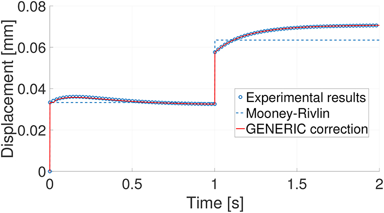
Figure 4. Comparison of the Mooney-Rivlin model prediction and its subsequent GENERIC correction with the experimental results for one particular experiment.
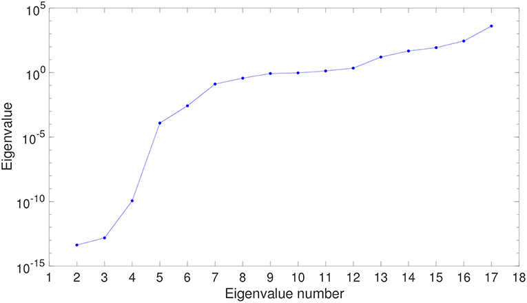
Figure 5. Evolution of the eigenvalues of the projection matrix in the embedding of experimental data. Only the first 17 eigenvalues are shown for clarity.
5.4. What if Some Terms Need no Correction?
Of course, in general we will not know in advance that a particular model is the best for the Hamiltonian part of the behavior. In a general situation both parts of the model will need to be corrected. To show the robustness of the presented method, we demonstrate here that if we try to correct the Hamiltonian part of the model, the method is able to detect that it is already correct (Mooney-Rivlin) and that it needs no correction. The method proceeds by correcting the dissipative part only, obtaining the same levels of error as the preceding section.
5.5. Constructing the Good Model
The final goal of the method is not to reproduce each one of the experimental results, but to be able to construct a true model from data. To this end, we first unveil the underlying manifold structure of the experimental data. The temporal series of zexp(t) is grouped into a high dimensional vector, one for each of the 557 experiments. These are then embedded, by means of Locally Linear Embedding techniques (Roweis and Saul, 2000) onto a low-dimensional manifold. This permits to unveil the true neighborhood structure between experimental data and, notably, to perform rigorous interpolation on the manifold structure—and not on the Euclidean space—among data.
The first step when applying LLE techniques to a set of high-dimensional data is to find the right dimensionality of the embedding space. To do so, the eigenvalues of the projection matrix are usually studied. These are depicted in Figure 5.
The first LLE eigenvalue is always close to zero within machine precision, and is discarded. The next “isolated” eigenvalues represent the true dimensionality of the embedding space (in this case, three). The rest of the eigenvalues are usually much closer to each other and do not represent the right dimensionality of the embedding space. Therefore, it seems that the right dimensionality of the embedding space is three—even two.
Locally Linear Embedding techniques need some user intervention to determine, by trial and error, the adequate number of neighbors for each datum. In this case we assume some 20 neighbors for each one. The key step in finding the good low-dimensional embedding of the data is to find a vector of weights W that minimizes the functional
Once these weights are found, LLE assumes that they continue to be valid in the low-dimensional embedding, and looks for the new coordinates ξ in this space accordingly, by minimizing a new functional
This procedure allows us to find the constitutive manifold, as defined in Ibañez et al. (2017). It is shown in Figure 6. The objective of this validation procedure will be to try to reproduce a control point in the manifold—a complete loading history, in fact—by obtaining its GENERIC model from the neighboring experimental points. This control point is shown in red in Figure 6.
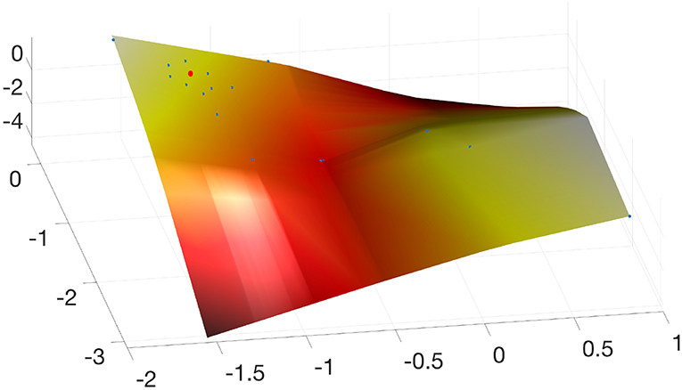
Figure 6. Obtained constitutive manifold by embedding the experimental results onto a three-dimensional space. Only a portion of the 557 experimental results are shown for clarity. In red, control point employed to validate the approach. Note that it is surrounded by a user-defined number of neighbors, whose GENERIC model is employed to obtain, by interpolation by means of the LLE weights, the sought model.
In Figure 7 the result of the interpolated model (in continuous line) and the eight neighboring experimental results (dashed lines) that served to construct the final GENERIC model for the red point in Figure 6 are shown. The mean squared error with respect to the control experimental history resulted be 0.174%.
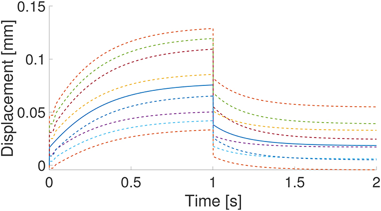
Figure 7. Result (continuous line) of the interpolation on the constitutive manifold of the eight neighboring experimental results (in dashed line). These are the time history of the eight neighboring points in Figure 6.
5.6. Full Model Correction
In the preceding sections we assumed that the Hamiltonian part of the model (basically, a Mooney-Rivlin model) was known and that the model needed only some amendment in its dissipative part. In this section we study the performance of the proposed technique if every term in the assumed model is wrong.
To this end, we assume for the solid a Neo-Hookean model with no viscous dissipation. The neo-Hookean model is basically equal to Mooney-Rivlin, see Equation (8), with C2 = 0. To make things even more difficult, we assume a bad calibration of the instruments so that, for this “wrong” model, C1 = 68.9 MPa (four times the right value for the Mooney-Rivlin model—the actual one—) and D1 = 0.0016.
Proceeding like in previous sections, we first computed corrections for each one of the 557 different experimental time series. For one of these essays, the prediction given by the “wrong” (neo-Hookean) model, the experimental results (coming from the Mooney-Rivlin model) and the corresponding corrected model predictions are shown in Figure 8.
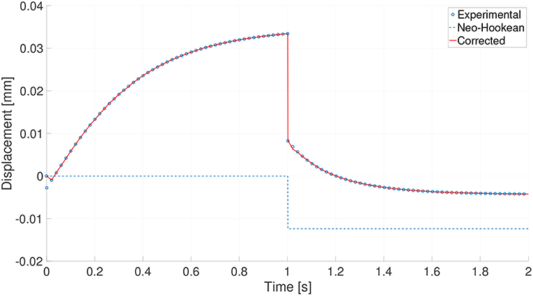
Figure 8. Experimental results (circles), prediction made by the neo-Hookean model (dashed line) and corrected model (red line) for experiment number 85.
For this particular case (every experiment provided similar results), the initial error for the prediction given by the “wrong” neo-Hookean model was 13.05%. After correction, the relative mean square error in the time history was 0.092%.
Once the whole 557 experiments have been corrected, the constitutive manifold for this material can be constructed by LLE methods, as detailed in Section 5.5.
With this constitutive manifold thus constructed we can now evaluate the behavior of any new strain-stress state by simply locating it in the manifold, determining its surrounding neighbors, and employing the LLE weights to interpolate its GENERIC terms. This was done for one of the experimental results, that was removed from the manifold for control purposes, and interpolated from its neighbors. The result of this process is shown in Figure 9.
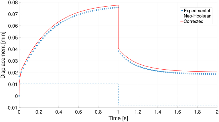
Figure 9. Experimental results (circles) for a new experiment, prediction made by the neo-Hookean model (dashed line) and interpolated corrected model (red line). The interpolation is made by employing the same weights provided by LEE techniques in constructing the constitutive manifold.
The mean squared error along the time history with respect to the control experiment was 1.057%.
6. Discussion
From the results just presented, it is clear that the proposed technique presents an appealing alternative for the machine learning of models from data. Instead of constructing data-driven models from scratch, constructing only corrections to existing, well-known models has shown to provide very accurate results that very much improve these models.
One key ingredient in these developments is the concept of constitutive manifold, that allows to interpolate experimental results in the right manifold structure. Existing works choose simply the nearest experimental neighbor, but, notably, this neighborhood is found in an Euclidean space (Kirchdoerfer and Ortiz, 2016) or in a Mahalanobis space (Ayensa-Jiménez et al., 2018).
The presented method is robust even if some parts of the model need no correction. The final method, as has been presented, has the important property of being sound from the thermodynamic point of view, guaranteeing, thanks to its GENERIC structure, the conservation of energy and positive production of entropy.
From the numerical point of view, the resulting, GENERIC-based time integrator schemes have already demonstrated their ability to conserve the right symmetries of the system (see, for instance, Romero, 2009 or González et al., 2018). In sum, we believe that the just presented technique, that should be extended to other types of systems, presents a promising future.
Data Availability Statement
The datasets [GENERATED/ANALYZED] for this study will be available upon request.
Author Contributions
DG, FC, and EC contributed in the conception and design of the study. DG coded the Matlab program. EC wrote the first draft of the manuscript. All authors contributed to manuscript revision, read and approved the submitted version.
Funding
This work has been supported by the Spanish Ministry of Economy and Competitiveness through Grants number DPI2017-85139-C2-1-R and DPI2015-72365-EXP and by the Regional Government of Aragon and the European Social Fund, research group T24 17R.
Conflict of Interest Statement
The authors declare that the research was conducted in the absence of any commercial or financial relationships that could be construed as a potential conflict of interest.
References
Ayensa-Jiménez, J., Doweidar, M. H., Sanz-Herrera, J. A., and Doblaré, M. (2018). A new reliability-based data-driven approach for noisy experimental data with physical constraints. Comp. Methods Appl. Mech. Eng. 328, 752–774. doi: 10.1016/j.cma.2017.08.027
Brunton, S. L., Proctor, J. L., and Kutz, J. N. (2016). Discovering governing equations from data by sparse identification of nonlinear dynamical systems. Proc. Natl. Acad. Sci. U.S.A. 113, 3932–3937. doi: 10.1073/pnas.1517384113
García, A., Martínez, M. A., and Peña, E. (2012). Viscoelastic properties of the passive mechanical behavior of the porcine carotid artery: Influence of proximal and distal positions. Biorheology 49, 271–288. doi: 10.3233/BIR-2012-0606
González, D., Chinesta, F., and Cueto, E. (2018). Thermodynamically consistent data-driven computational mechanics. Cont. Mech. Thermodyn. 1–15. doi: 10.1007/s00161-018-0677-z
Grmela, M., and Oettinger, H. C. (1997). Dynamics and thermodynamics of complex fluids. I. development of a general formalism. Phys. Rev. E. 56, 6620–6632. doi: 10.1103/PhysRevE.56.6620
Grosse, R. B., Salakhutdinov, R., Freeman, W. T., and Tenenbaum, J. B. (2012). “Exploiting compositionality to explore a large space of model structures,” in Proceedings of the Twenty-Eighth Conference on Uncertainty in Artificial Intelligence, UAI'12, (Arlington, VA: AUAI Press), 306–315.
Holzapfel, G. A. and Gasser, T. C. (2000). A new constitutive framework for arterial wall mechanics and a comparative study of material models. J. Elastic. 61, 1–48. doi: 10.1023/A:1010835316564
Ibañez, R., Abisset-Chavanne, E., Gonzalez, D., Duval, J., Cueto, E., and Chinesta, F. (2018). Hybrid constitutive modeling: data-driven learning of corrections to plasticity models. Int. J. Mat. Forming. doi: 10.1007/s12289-018-1448-x. [Epub ahead of print].
Ibañez, R., Borzacchiello, D., Aguado, J. V., Abisset-Chavanne, E., Cueto, E., Ladeveze, P., et al. (2017). Data-driven non-linear elasticity: constitutive manifold construction and problem discretization. Comput. Mech. 60, 813–826. doi: 10.1007/s00466-017-1440-1
Kirchdoerfer, T., and Ortiz, M. (2016). Data-driven computational mechanics. Comp. Methods Appl. Mech. Eng. 304, 81–101. doi: 10.1016/j.cma.2016.02.001
Kirchdoerfer, T., and Ortiz, M. (2017a). Data-driven computing in dynamics. Int. J. Numer. Meth. Eng. 113, 1697–1710. doi: 10.1002/nme.5716
Kirchdoerfer, T., and Ortiz, M. (2017b). Data driven computing with noisy material data sets. Comp. Methods Appl. Mech. Eng. 326, 622–641. doi: 10.1016/j.cma.2017.07.039
Lake, B. M., Ullman, T. D., Tenenbaum, J. B., and Gershman, S. J. (2017). Building machines that learn and think like people. Behav. Brain Sci. 40:e253. doi: 10.1017/S0140525X16001837
Lam, R. R., Horesh, L., Avron, H., and Willcox, K. E. (2017). Should you derive, or let the data drive? an optimization framework for hybrid first-principles data-driven modeling. arXiv:1711.04374.
Latorre, M., and Montáns, F. J. (2014). What-you-prescribe-is-what-you-get orthotropic hyperelasticity. Comput. Mech. 53, 1279–1298. doi: 10.1007/s00466-013-0971-3
Lopez, E., Gonzalez, D., Aguado, J. V., Abisset-Chavanne, E., Cueto, E., Binetruy, C., et al. (2018). A manifold learning approach for integrated computational materials engineering. Arch. Comput. Meth. Eng. 25, 59–68. doi: 10.1007/s11831-016-9172-5
Mihai, L. A., and Goriely, A. (2017). How to characterize a nonlinear elastic material? a review on nonlinear constitutive parameters in isotropic finite elasticity. Proc. R. Soc. Lond. A Math. Phys. Eng. Sci. 473. doi: 10.1098/rspa.2017.0607
Millán, D., and Arroyo, M. (2013). Nonlinear manifold learning for model reduction in finite elastodynamics. Comp. Meth. Appl. Mech. Eng. 261–262, 118–131. doi: 10.1016/j.cma.2013.04.007
Öttinger, H. C. (2012). Nonequilibrium thermodynamics: a powerful tool for scientists and engineers. DYNA 79, 122–128. doi: 10.3929/ethz-a-010744301
Peherstorfer, B., and Willcox, K. (2015). Dynamic data-driven reduced-order models. Comp. Metho. Appl. Mech. Eng. 291, 21–41. doi: 10.1016/j.cma.2015.03.018
Peherstorfer, B., and Willcox, K. (2016). Data-driven operator inference for nonintrusive projection-based model reduction. Comp. Meth. Appl. Mech. Eng. 306, 196–215. doi: 10.1016/j.cma.2016.03.025
Peña, J., Martínez, M., and Peña, E. (2011). A formulation to model the nonlinear viscoelastic properties of the vascular tissue. Acta Mech. 217, 63–74. doi: 10.1007/s00707-010-0378-6
Raissi, M., Perdikaris, P., and Karniadakis, G. E. (2017a). Physics informed deep learning (part i): data-driven solutions of nonlinear partial differential equations. arXiv:1711.10561.
Raissi, M., Perdikaris, P., and Karniadakis, G. E. (2017b). Physics informed deep learning (part ii): data-driven discovery of nonlinear partial differential equations. arXiv:1711.10566.
Romero, I. (2009). Thermodynamically consistent time-stepping algorithms for non-linear thermomechanical systems. Int. J. Numer. Methods Eng. 79, 706–732. doi: 10.1002/nme.2588
Romero, I. (2010). Algorithms for coupled problems that preserve symmetries and the laws of thermodynamics: Part i: Monolithic integrators and their application to finite strain thermoelasticity. Comp. Meth. Appl. Mech. Eng. 199, 1841–1858. doi: 10.1016/j.cma.2010.02.014
Romero, I. (2013). A characterization of conserved quantities in non-equilibrium thermodynamics. Entropy 15, 5580–5596. doi: 10.3390/e15125580
Roweis, S. T., and Saul, L. K. (2000). Nonlinear dimensionality reduction by locally linear embedding. Science 290, 2323–2326. doi: 10.1126/science.290.5500.2323
Swischuk, R., Mainini, L., Peherstorfer, B., and Willcox, K. (2018). Projection-based model reduction: formulations for physics-based machine learning. Comp. Fluids. doi: 10.1016/j.compfluid.2018.07.021. [Epub ahead of print].
Tenenbaum, J. B., de Silva, V., and Langford, J. C. (2000). A global framework for nonlinear dimensionality reduction. Science 290, 2319–2323. doi: 10.1126/science.290.5500.2319
Keywords: data-driven computational mechanics, hyperelasticity, model correction, GENERIC, machine learning
Citation: González D, Chinesta F and Cueto E (2019) Learning Corrections for Hyperelastic Models From Data. Front. Mater. 6:14. doi: 10.3389/fmats.2019.00014
Received: 05 November 2018; Accepted: 25 January 2019;
Published: 15 February 2019.
Edited by:
Christian Johannes Cyron, Technische Universität Hamburg, GermanyReviewed by:
Kevin Linka, Technische Universität Hamburg, GermanyYouyong Li, Soochow University, China
Copyright © 2019 González, Chinesta and Cueto. This is an open-access article distributed under the terms of the Creative Commons Attribution License (CC BY). The use, distribution or reproduction in other forums is permitted, provided the original author(s) and the copyright owner(s) are credited and that the original publication in this journal is cited, in accordance with accepted academic practice. No use, distribution or reproduction is permitted which does not comply with these terms.
*Correspondence: Elías Cueto, ecueto@unizar.es