Reconstruction of daily chlorophyll-a concentrations in the transit of severe tropical cyclone Hudhud using the ExDINEOF method

1 Introduction

Chlorophyll-a concentration data hold significance across diverse scientific domains, including global climate change, the global carbon cycle, biogeochemical cycles, and water quality (Maeda et al., 2019; Ma et al., 2021). Ocean-color remote sensing offers advantages over traditional methods for measuring chlorophyll-a concentrations. However, multiscale optical remote sensing data often suffer from extensive data gaps. The absence of chlorophyll-a concentration data hampers research on marine life’s geochemical cycles and global climate change. In tropical regions, persistent cloud cover exacerbates this issue, necessitating data reconstruction to bridge these gaps.

The presence of widespread data irregularities and sparsity significantly impedes the progress of ocean-color remote sensing. Consequently, addressing missing data through reconstruction has emerged as a pivotal research aspect. Numerous researchers have explored data reconstruction methods (Jayaram et al., 2018; Ji et al., 2018; Liu and Wang, 2018; Yu et al., 2019). Optimum interpolation (OI) and data interpolating empirical orthogonal function (DINEOF) methods are commonly used in ocean-color remote sensing data reconstruction and use empirical orthogonal functions (Bretherton et al., 1976; Alvera-Azcárate et al., 2005; Reynolds and Smith, 1994; Waite and Mueter, 2013; Novelli et al., 2016). DINEOF, a parameter-free interpolation technique, was initially proposed by Beckers and Rixen (2003). This method employs empirical orthogonal function decomposition to reconstruct missing data in time series, enhancing efficiency and performance for datasets with substantial missing data and extended time series. Thus, DINEOF has been increasingly used in diverse applications (Beckers and Rixen, 2003; Alvera-Azcárate et al., 2009; Li and He, 2014). The DINEOF technique establishes a model grounded in historical data within a time series of a singular variable, subsequently enabling the prediction of absent data. However, this approach falls short in reconstituting the spatio-temporal domain data when the extent of valid data coverage is exceedingly minimal (less than 2%) (Alvera-Azcárate et al., 2015). If DINEOF is employed to reconstruct these regions, the outcome will be the average value extracted from historical time-series datasets, which would not accurately depict the authentic spatio-temporal distribution. Consequently, during practical applications, raw data marked by a high proportion of absent data tends to be excluded. This, in turn, constrains the applicability of this method within regions where data availability is scant.

While many studies investigate the reconstruction of environmental factors like sea surface temperature (SST) (Bignami et al., 2007; Zhao and He, 2012; Shropshire et al., 2016; Ji et al., 2018; Ma et al., 2021), wind field(Jayaram et al., 2014), turbidity(Alvera-Azcárate et al., 2015), sea surface salinity (SSS) (Alvera-Azcárate et al., 2016), and total suspended matter (NeChad et al., 2011)in ocean-color remote sensing, reconstruction methods for chlorophyll-a concentration data, crucial for global climate change and biogeochemical cycles, remain underdeveloped and warrant further exploration (Gunes et al., 2008; NeChad et al., 2011; Waite and Mueter, 2013). Most studies focus on regions with fewer missing data, such as the Mediterranean Sea (Alvera-Azcárate et al., 2005; Beckers et al., 2006; Antoine et al., 2008; Brando et al., 2015), the northern South China Sea (Ping et al., 2016; Ma et al., 2021), and the North Atlantic Ocean (Everson et al., 1996; Iida and Saitoh, 2007; Xiu et al., 2007; Zhao and He, 2012; Jouini et al., 2013; Waite and Mueter, 2013; Li and He, 2014; Wang and Liu, 2014; Liu and Wang, 2016; Shropshire et al., 2016; Hilborn and Costa, 2018; Wang et al., 2019). However, regions influenced by tropical monsoons or tropical rainy climates, where data scarcity is significant, have received limited attention, like the Bay of Bengal and its environs (Sirjacobs et al., 2011; Park et al., 2013). Temporal resolution also factors into ocean-color data reconstruction. While common reconstruction methods demand sufficient sample data points, current studies on chlorophyll-a concentration data reconstruction typically employ monthly-scale data (Wang and Liu, 2014; Yu et al., 2019). Notably, recent years have witnessed the use of an 8-day scale for ocean-color data reconstruction, generally yielding favorable outcomes (Jayaram et al., 2018; Martinez et al., 2020; Jayaram et al., 2021). Although some investigations have explored global-scale daily-scale data reconstruction (Liu and Wang, 2018; Liu and Wang, 2019), the approach’s application on small-to-medium spatial scales remains limited, especially within tropical regions. The rapid generation and dissipation of sea surface chlorophyll-a concentration features, occurring in as little as three days for phytoplankton, accentuate the inadequacy of monthly-scale data for research needs. Consequently, there is an imminent requirement for higher temporal resolution reconstructed data to analyze biogeochemical cycles.

To summarize, current data reconstruction methods primarily rely on historical data of a single variable to establish models and predict missing data for different time periods and regions. In terms of research focus, most studies concentrate on reconstructing SST data, with only a small proportion addressing the reconstruction of missing chlorophyll-a concentration data in remote sensing (Xiao et al., 2019). While research areas for data reconstruction typically involve temperate waters, the challenge escalates in tropical seas due to increased cloud cover and rainfall. Existing works on chlorophyll-a concentration data reconstruction are predominantly conducted on a monthly or 8-day scale, rather than a daily scale (Wang et al., 2019). To capture short-term changes in the ocean environment of tropical oceans, daily-scale long-time-series remote-sensing chlorophyll-a concentration data is imperative. However, the presence of persistent clouds in tropical regions poses a significant hindrance to reconstruction efforts. Furthermore, while a few studies focus on an 8-day scale reconstruction, daily-scale data reconstruction is scarce. Researchers assert that studies on chlorophyll-a concentration data reconstruction should target large-scale, long-time-series data in regions significantly impacted by cloud cover. Nonetheless, the reconstruction of daily data within small-to-medium areas also warrants attention (Pottier et al., 2008; De Montera et al., 2011; Jouini et al., 2013). Thus, conducting a combined multivariate reconstruction of daily chlorophyll-a concentration data in small and medium regions, particularly in typical tropical waters like the Bay of Bengal, holds practical significance, theoretical value, and urgency.

Several studies have utilized the multivariate OI method for data reconstruction. For instance, Reynolds et al. (1994) employed the OI approach to integrate inverted SST using the Advanced Very High Resolution Radiometer (AVHRR) and actual SST measured by boats or buoys. This successfully produced widely used daily and weekly average temperature analysis products globally (Reynolds and Smith, 1994). Grodsky and Carton (2001) utilized sea surface height (SSH) and the mixing layer rate to validate near-surface currents in the tropical Pacific Ocean (Grodsky and Carton, 2001). These studies demonstrated that employing multiple variables in data reconstruction yields more realistic reconstructed data. Despite the advantages of the OI approach, such as practical interpolation and reduced computational costs, it selectively employs adjacent information for interpolation calculations. This process is subjective and does not objectively estimate covariance between variables or obtain the error statistics needed for OI analysis. In contrast, the DINEOF method establishes relationships within inherent available data for variable reconstruction, eliminating the need for subjective parameter estimation. However, the traditional DINEOF method has limitations, filling missing data solely based on the inherent spatiotemporal relationship of a single variable. When dealing with extensive missing data areas, inadequate samples result in unreliable outcomes. Alvera-Azcárate et al. extended the traditional DINEOF method as ExEOFs in the West Florida Shelf. By incorporating environmental factors like SST, chlorophyll-a, and wind field within a specific space-time region, this improved ExEOFs method effectively reconstructed missing SST data. Comparative analysis with actual SST measurements revealed that the ExEOFs method achieved notably higher accuracy than the traditional monovariate DINEOF method (Alvera-Azcárate et al., 2007). Addressing DINEOF’s limitations in reconstructing daily data in tropical seas with high missing data quantities, this study employs an adapted multivariate ExDINEOF method. This approach utilizes combinations of parameters closely linked to chlorophyll-a concentration, including SST, SSH, SSS, and wind field, to reconstruct missing data.

The paper’s structure is as follows. Section 2 introduces the study area, data, and methodology. Section 3 discusses the results and data reconstruction validation. Further commentary and conclusions are presented in Sections 4 and 5, respectively.

2 Materials and methods

2.1 Study area

The study area encompasses the Bay of Bengal (Figure 1), situated between 5°–24°N and 79°–123°E. The climate in this region predominantly constitutes tropical oceanic monsoon type, featuring minor variations in daily and annual temperatures. Observed SST averages fall within the range of 25–29°C, with an estimated annual temperature range of about 6°C (Roxy et al., 2014; Thompson et al., 2017). Notably, the average humidity exceeds 80%, and annual precipitation ranges from 1500–2000 mm. This climate pattern results in frequent cloud cover, particularly during the rainy season, posing challenges for optical remote sensing. The study area stands out for its sparse chlorophyll-a concentration data records. Moreover, the Bay of Bengal is among the world’s most active tropical cyclone regions. Consequently, investigating missing data reconstruction in this tropical region holds both practical significance and theoretical value.

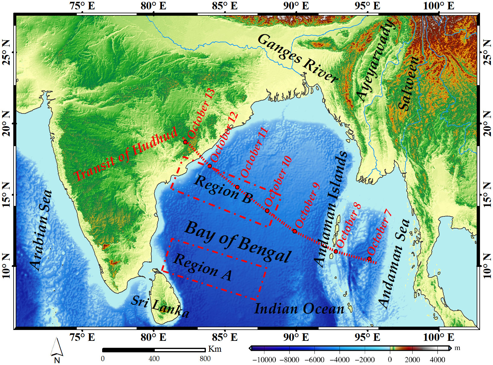
Figure 1 Study area and the path of the severe tropical cyclone Hudhud. Region A covers the area 9°–12°N and 80°–88°E, and Region B covers the area 16°N and 80°–88°E.

2.2 The severe tropical cyclone Hudhud

On October 7, 2014, the severe tropical cyclone Hudhud developed in the Andaman Sea, subsequently traversing the Andaman Islands toward the Bay of Bengal (Figure 1) (Chacko, 2017). Hudhud brought substantial cloud cover, leading to widespread missing data in daily chlorophyll-a concentration records. Given the brief duration of tropical cyclones, daily data reconstruction proves invaluable in illustrating spatial and temporal chlorophyll-a concentration patterns during short-term cyclones or typhoons. Notably, the reconstruction of daily chlorophyll-a concentration data in the tropical study area around the time of severe tropical cyclone Hudhud encountered formidable challenges.

2.3 Data

Level-3 integrated daily chlorophyll-a concentration data, generated using the OC5 algorithm (ChlOC5) (Gohin et al., 2010), were combined with Level 2 ChlOC5 data from various sensors: the Medium Resolution Imaging Spectrometer, the MODerate Resolution Imaging Spectroradiometer, the Sea-Viewing Wide Field Sensor, the Visible and Infrared Imaging Radiometer Suite, and the Ocean and Land Color Instrument. The spatial resolution of Level-3 integrated data was 4 km (Table 1). As depicted in Figure 2A, multi-year average data coverage in the study area exhibits significant variability. Most areas in the region of interest feature data coverage of around 25-35%, with notably low coverage of approximately 10-15% in the estuarine coastal zone (Figure 2A). Data coverage in October 2014 varies widely, ranging from 3.92% to 82.88%, with a 31-day average coverage of 39.13% (Figure 2B). The presence of only a limited 31-day dataset in a tropical sea area with persistent data scarcity throughout the year presents considerable challenges for data reconstruction studies.

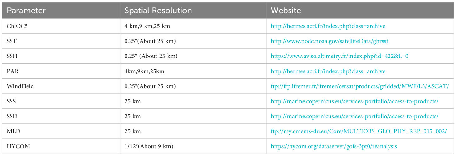
Table 1 The data sources used in this study.

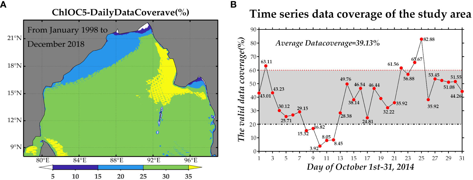
Figure 2 Multi-year (January 1, 1998 - December 31, 2018) average ChlOC5 data coverage (A) and 31-day ChlOC5 data coverage in October 2014 (B).

Besides, the wind field data of the advanced scatterometer, the photosynthetically available radiation (PAR) data, and the thermal infrared and microwave remote-sensing data from satellite observations of the SST, the SSS, the sea surface density (SSD), the mixed layer depth (MLD), and the SSH were analyzed in this study (Table 1). Moreover, the Hybrid Coordinate Ocean Model (HYCOM) reanalysis data, combining remote-sensing, in-situ measured, and model-simulated datasets, were utilized, encompassing SST, SSS, SSH, Eastward Sea Water Velocity (U-velocity), and Northward Sea Water Velocity (V-velocity) parameters (Table 1). Table 1 details the spatial resolutions of the datasets, ranging from 4 km to 25 km for ChlOC5 and PAR data, and 0.25° for SST, SSH, SLA, Wind Speed, and Wind Stress. The resolution for MLD, SSS, and SSD data is 25 km, while HYCOM reanalysis data has a resolution of 1/12°. All datasets, as shown in Table 1, are formatted in Network Common Data Form (NetCDF) format. For easier processing, ChlOC5 and PAR data were resampled to 9 km in MATLAB 2018. Subsequently, all data were integrated into a 3D dataset in MATLAB 2018 for subsequent reconstruction steps, marking the completion of data preprocessing.

2.4 Methods

Marine physical environmental factors, such as SST, wind, sea surface flow field, SSH, and sea-surface chlorophyll-a concentration data, are all impacted by atmospheric and marine dynamics (Figure 3). These factors are inherently interconnected, enabling the utilization of these connections to reconstruct missing data. However, disparities exist between the reconstructed chlorophyll-a concentration data and data reconstructed from other environmental parameters.

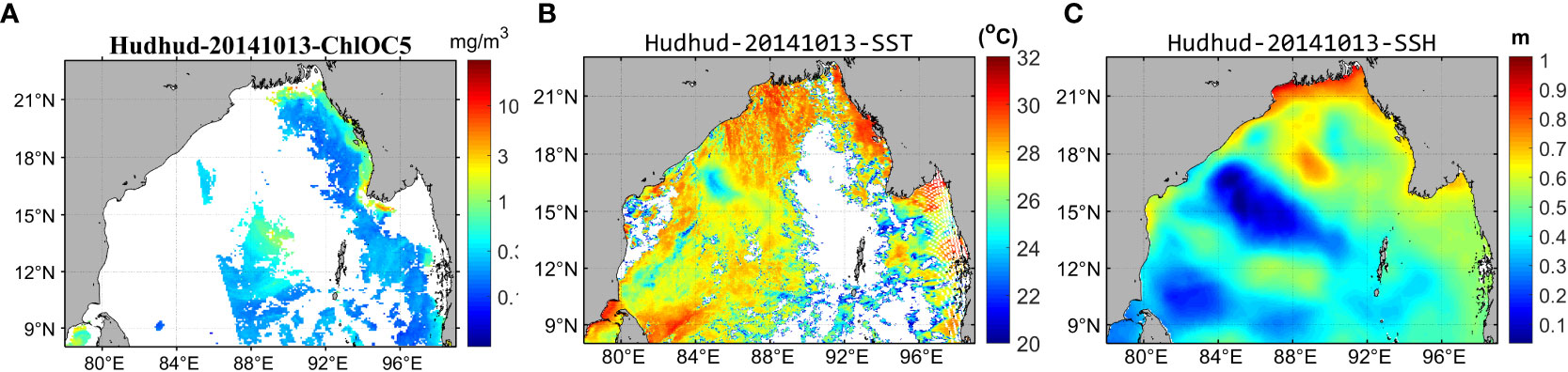
Figure 3 Comparison of data coverage for chlorophyll-a concentration (A), SST (B), and SSH (C).

2.4.1 Difficulties in reconstructing daily chlorophyll-a concentration in tropical ocean during the transit of severe tropical cyclones

Research efforts have primarily concentrated on reconstructing missing SST data. Notably, chlorophyll-a concentrations significantly impact global climate change and biogeochemical cycles. However, studies on chlorophyll-a concentration reconstruction remain in their nascent stages. This is due to several factors. Firstly, sea surface chlorophyll-a concentrations are influenced by numerous environmental variables, with their spatial and temporal variability, as well as data distribution irregularities, surpassing those of parameters such as SST and salinity. Moreover, the wavelengths used for chlorophyll-a concentration inversion in remote sensing primarily fall within the blue-green spectrum, susceptible to cloud cover, aerosols, water vapor, and sun glint. Additionally, limitations of inversion algorithms and the influence of turbid waters near shorelines contribute to larger areas of missing chlorophyll-a concentration data compared to other parameters. Consequently, the inversion of sea surface chlorophyll-a concentration data poses greater challenges. These challenges result in extensive missing areas in chlorophyll-a concentration data due to algorithmic effects and cloud interference, leading to inadequate sample sizes for effective reconstruction.

Several complexities emerge when undertaking reconstitution studies for daily chlorophyll-a concentration products in the study area. Initially, the study reconstructed daily-scale chlorophyll-a concentration data in the tropical oceanic region during the transit of severe tropical cyclones. Notably, from October 8 to 12, 2014, when robust tropical cyclones passed through the study area, data coverage remained slightly below 20%. Particularly, data coverage stood at merely 3.92%, 8.05%, and 8.45% for October 10-12, respectively. Secondly, the ExDINEOF method did not incorporate lagged version data, resulting in a reduced sample size. Severe data deficiencies stem from three key factors: tropical marine regions, small and medium spatial scales, and abbreviated time series durations. Even with the inclusion of lagged data, insufficient reference information persists, hindering the reconstruction of missing data points. Thirdly, only 31 days of daily chlorophyll-a concentration data, in contrast to the 180 days utilized for SST reconstruction (Alvera-Azcárate et al., 2007), were employed for reconstructing the daily missing data. This limitation arises due to the brief duration of strong tropical cyclone transit, lasting barely a week. Utilizing data from an extensive time series would result in low-pass filtered outcomes, owing to the Empirical Orthogonal Function (EOF) effect.

2.4.2 The ExDINEOF method

Alvera-Azcárate and colleagues (2007) initially expanded the mono-variate DINEOF method to reconstruct absent SST data in the coastal region of the Gulf of Mexico. The outcomes demonstrated that the extended EOFs (ExEOFs) achieved greater precision than the mono-variate DINEOF. The reconstructed chlorophyll-a concentration data exhibits distinct attributes. Multiple environmental elements, including aerosols, thin clouds, fog, extremely turbid Class-II waters, and sun glint, impact chlorophyll-a concentration data (Sravanthi et al., 2017). As outlined in Mie scattering theory, shorter wavelengths in the blue-green spectrum result in a more pronounced influence of these environmental factors on the chlorophyll-a concentration inversion algorithm (Wang et al., 2020). In contrast, SST measurements derived from thermal infrared inversion possess a larger valid data coverage area compared to chlorophyll-a concentration data, attributed to their longer wavelengths and day/night availability (Figure 3). Consequently, the spatio-temporal variability and irregular distribution of chlorophyll-a concentration data surpass those of SST data concerning data reconstruction (Figure 3). Therefore, this study eschewed extensive historical data sets and instead leaned towards the relationship between chlorophyll-a concentration and closely associated environmental factors to reconstruct missing data within a small and medium-sized spatial range in tropical ocean settings.

This section presently examines the connection between the chlorophyll-a concentration datasets and various environmental factors influencing the temporal and spatial fluctuations of short-term chlorophyll-a concentration cycles through the application of the ExDINEOF technique (Ji et al., 2018; Yu et al., 2019). The fundamental mathematical formulation of ExDINEOF can be outlined in the ensuing steps:

where X_ExDINEOF is the multivariate reconstruction array; a₁, a₂,…, a_N are the column vectors of the time series that contain all the space points in matrix a at times 1, 2,…, N. Matrices a, b, c, d, e, f, and g are the chlorophyll-a concentration data and the relevant environmental factors. The size of the matrices is estimated as: a = M×N, b = O×N, c = P×N, d = Q×N, e = R×N, f = S×N, and g = U×N, where M, O, P, Q, R, S, and U are the spatial dimensions of matrices a, b, c, d, e, f, and g, respectively; and N is the temporal dimension of each matrix. Specifically, for severe tropical cyclone Hudhud, the spatial matrices M, O, P, Q, R, S, and U cover the range 78–99°E and 8–23°N with around 263*189 spatial-dimension pixels (the data are resampled to obtain a 9-km resolution to enhance the computational efficiency). The numerical value of N in this context is 31. Consequently, the data pertaining to each of the seven variate products comprises a three-dimensional array containing 26318931 pixels. It should be noted that the spatial size of the matrices M, O, P, Q, R, S, and U can differ, but the numbers of their temporal dimensions must be identical. In this paper, the spatial matrices M, O, P, Q, R, S, and U all have the same size.

The datasets, which are stored in a matrix X_ExDINEOFand averaged in time and space, are subtracted beforehand. The missing data are initialized to zero to ensure that they are unbiased with respect to X_ExDINEOF. Utilizing the initial estimation, a first-order EOF is employed, denoted as (k = 1), for the purpose of executing the initial singular value decomposition (SVD). Subsequently, the absent data are substituted with the derived EOF in the subsequent manner:

Where i, j are the spatial and temporal indices of the missing data in matrix X_ExDINEOF; u_p and v_p are the pth columns of the spatial and temporal EOF U and V; ρ_P is the corresponding singular value, P = 1… k, and k is the number of EOF modes used for reconstruction, where k = 2,3,4,…, k_max, respectively. The SVD is iterated once more to incorporate the updated values for the absent data. These final two steps are reiterated until convergence is achieved in the values of the missing data. Subsequently, for each iteration index k, an approximation of the missing value is acquired. The most suitable count of EOFs to be retained for the purpose of reconstruction is determined through a cross-validation approach: a subset of data points (typically constituting 1% of the initial dataset) is pre-selected and designated as missing values. During each iteration of EOF estimation, the discrepancy between these initial points and their reconstructed counterparts is computed, allowing for the identification of the optimal number of EOFs that minimizes this discrepancy. Concurrently with the reconstructed dataset, a localized field of error is generated, reflecting the precision of the reconstruction. To enhance computational efficiency, the Lanczos method is employed within DINEOF to compute the empirical orthogonal functions (Alvera-Azcárate et al., 2007).

3 Results

3.1 Reconstructed daily chlorophyll-a concentration data for cyclone Hudhud in the tropical bay of Bengal

Figure 4 illustrates the spatial distribution of daily chlorophyll-a concentration data (ChlOC5) prior to, during, and subsequent to the occurrence of cyclone Hudhud spanning from October 1 to October 30, 2014. In the period preceding the cyclone’s occurrence (October 1–5, 2014, depicted in Figures 4A–C), a substantial expanse was occupied by daily data points that were missing. During the passage of cyclone Hudhud (October 7–13, shown in Figures 4D–G), the deficiency in data coverage became more severe, with a considerable area devoid of any data. As the cyclone traversed the region (as evidenced in Figures 4H–O), a substantial portion of data was still found to be absent, except for the case depicted in Figure 4M, where the data coverage was extensive. This absence of data coverage hindered the subsequent analysis of variations in chlorophyll-a concentration post the cyclone’s passage.

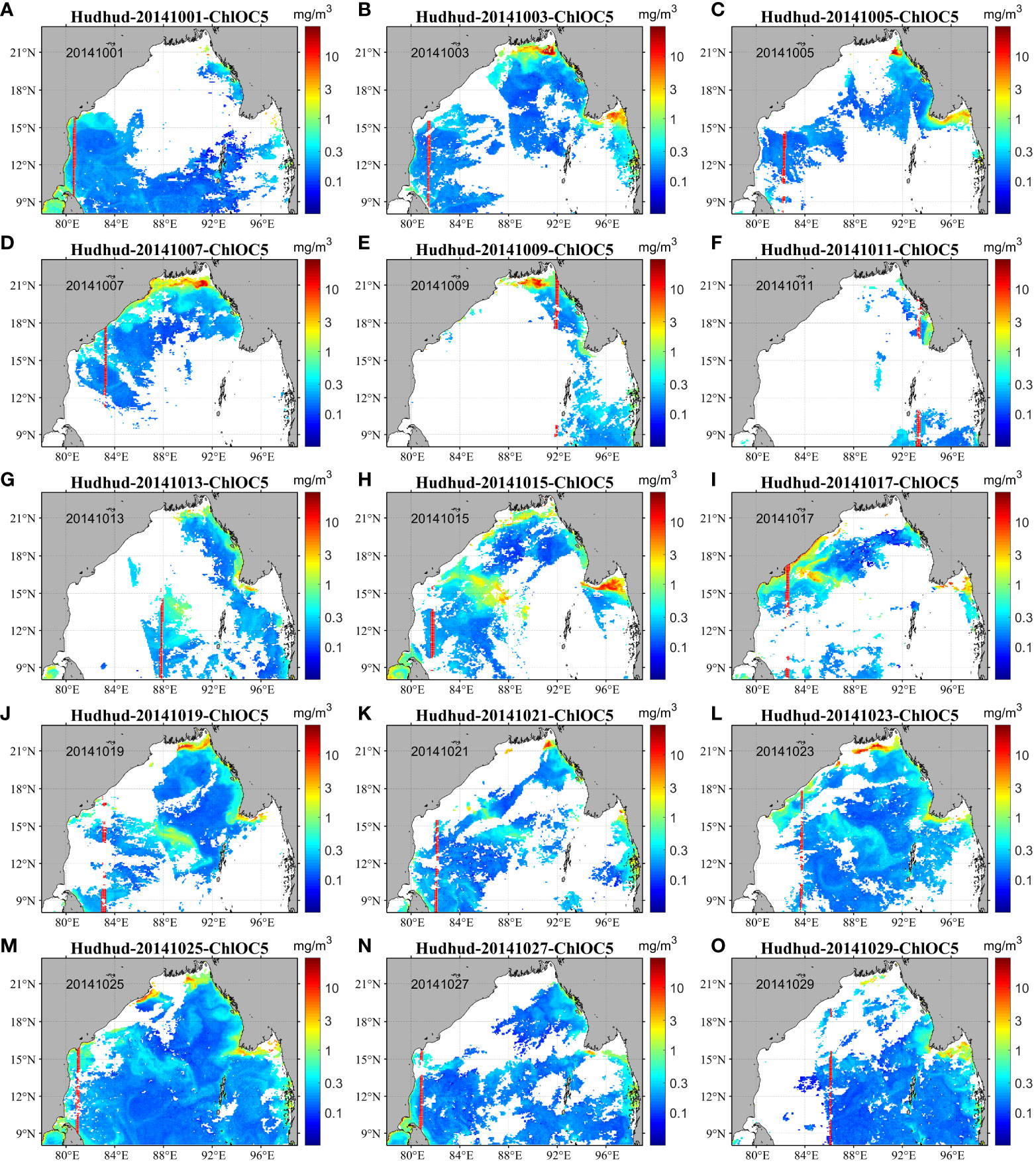
Figure 4 Original daily ChlOC5 chlorophyll-a concentration data before, during, and after passage of tropical cyclone Hudhud from October 1–30, 2014. (A–O) show the daily original ChlOC5 chlorophyll-a concentration data at an interval of two days from October 1–30, 2014. The distributions of randomly chosen data points for numbers 1001–1200 (200 data points in total) of the study area are shown as red points.

Figure 5 displays the daily reconstructed chlorophyll-a concentration data achieved through the implementation of the ExDINEOF technique. Upon scrutinizing the spatial arrangement, it can be observed that the reconstructed data effectively reinstated the situation of missing data across a substantial area. The outcomes of the reconstruction were determined to be comprehensive, devoid of any missing data points. Across the overall reconstruction, the values exceeded 1 mg/m³ within the northern coastal region of the Bay of Bengal, particularly at the Ganges River estuary. In certain extreme instances, the values even reached 3 mg/m³. In contrast, for vast offshore regions, the reconstructed values predominantly ranged from 0.1 to 0.3 mg/m³. Moreover, in the middle region of the Bay of Bengal, northwest of the Andaman Islands (as depicted in Figure 1), a significant striped area characterized by maximal chlorophyll-a concentrations was observable. On October 1, 2014, prior to the arrival of cyclone Hudhud, the chlorophyll-a concentration within the striped region was approximately 0.25 mg/m³ (Figure 5A), only slightly higher than that of neighboring areas. Additionally, the striped pattern with respect to chlorophyll-a concentration was not distinctly discernible. However, between October 3 and 7, an augmentation in chlorophyll-a concentration was evident in that region (Figures 5B–D). By October 13, when cyclone Hudhud made landfall (Figure 5G), the chlorophyll-a concentration had risen to approximately 2 mg/m³. Subsequently, the concentration continued to increase, reaching its pinnacle of around 3 mg/m³ (Figure 5I), after which it began to recede, stabilizing around 0.3 mg/m³. Ultimately, by October 29, the chlorophyll-a concentration further diminished to roughly 0.2 mg/m³.

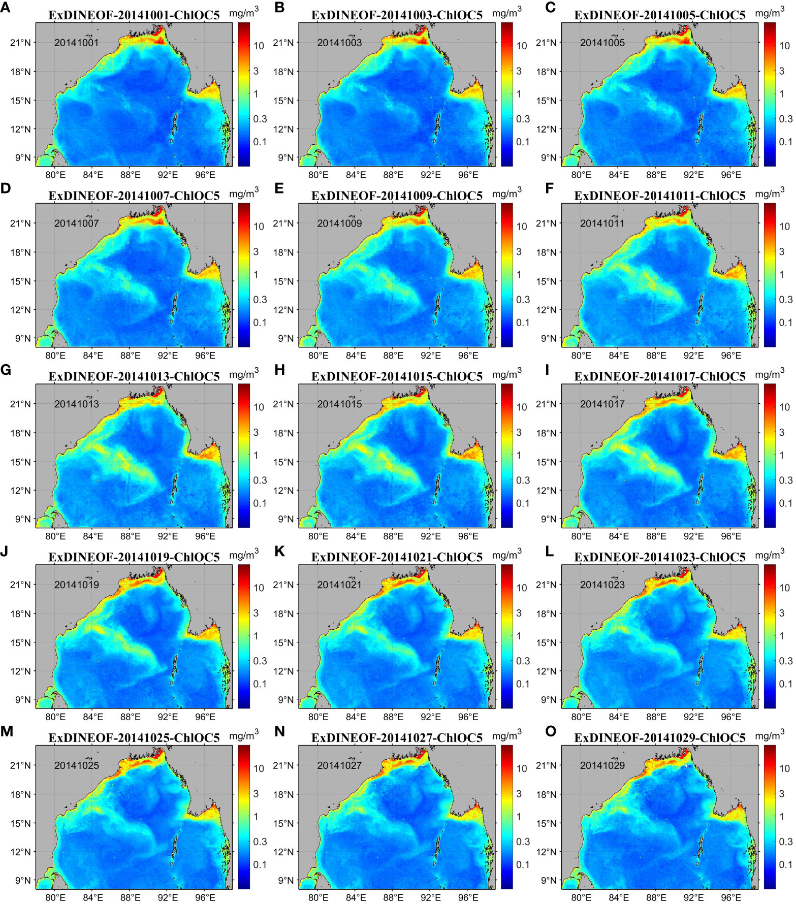
Figure 5 Daily ChlOC5 chlorophyll-a concentration data for the Bay of Bengal (October 2014) reconstructed using the ExDINEOF method. (A–O) show the daily ChlOC5 chlorophyll-a concentration data reconstructed using the ExDINEOF method at an interval of 2 days from October 1–30, 2014.

Upon analyzing the reconstructed data graph (Figure 5), it becomes apparent that near 90°E and 18°N, situated in the northern sector of the Bay of Bengal, a circular region characterized by low chlorophyll-a concentration began to take shape gradually from October 1 (Figures 5A–F). Between October 15 and 19, this circular pattern became distinctly evident, exhibiting a peripheral chlorophyll-a concentration of approximately 0.1 mg/m³. The central portion of the circle manifested a slightly elevated chlorophyll-a concentration ranging from 0.2 to 0.3 mg/m³ (Figures 5H–J). This circular pattern persisted until October 29 (Figure 5O).

By comparing Figures 4 and 5, it can be inferred that the ExDINEOF methodology exhibited commendable efficacy in reconstructing the daily missing data within confined regions both before and after the occurrence of tropical cyclone Hudhud. The deficient chlorophyll-a concentration data within the time series were adequately reconstructed within local contexts, whether preceding, during, or succeeding the cyclone’s passage. Furthermore, the formation and dissipation of the circular region characterized by lower chlorophyll-a concentration, which would have remained obscured due to data gaps in the initial dataset, were clearly elucidated. This successful demonstration further attests to the practicality of the ExDINEOF reconstruction approach.

3.2 Comparison of the spatial distribution of the reconstructed results using alternative methods

To further evaluate the method’s efficacy, namely the ExDINEOF method, alongside DINEOF and the bidirectional autoregressive model (BAR) approaches, were utilized to reconstruct variations in chlorophyll-a concentrations within the study region during and subsequent to the passage of the rapidly changing typhoon. A comparison of the methods was performed based on the spatial distribution of the reconstructed outcomes.

The bidirectional autoregressive model (BAR) employed in this research entails the repetition of forward and backward time-series vectors within MATLAB. The values of the reconstructed missing-like metadata are determined via calculating the mean values of both the forward and backward autoregressive models (Zhang et al., 2009). It can be discerned from Figure 6 that the correlation coefficient between times T and T+1 for chlorophyll-a concentration stands at 0.72, surpassing the requisite threshold of 0.5. As such, the essential prerequisites for BAR data reconstruction are fulfilled.

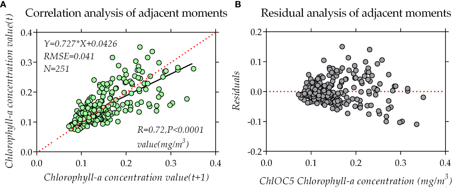
Figure 6 Correlation and residual analysis of chlorophyll-a concentration data at adjacent times: (A) Correlation of chlorophyll-a concentration data at times T and T+1 of the time series. (B) Residual distribution of the correlation of the time-series data between adjacent times.

Through the application of the EOF approach, the reconstructed chlorophyll-a values within the region of missing data undergo iterative decomposition and synthesis until the cross-validated error attains its minimum. The optimal eigenmode retention is then ascertained, aligning with the most effective reconstruction of data. The time series of daily chlorophyll-a concentrations data for the study area was preprocessed using MATLAB and organized into a three-dimensional m×n matrix, where m signifies the daily ChlOC5 data within the study region (spatial, two-dimensional), and n denotes the count of time series ChlOC5 data points (temporal, one-dimensional). For the purpose of extracting oceanic pixels, a land mask was applied to the m×n matrix. Subsequently, the DINEOF package was employed on this matrix to complete the missing daily chlorophyll-a ChlOC5 data.

Figure 7 illustrates the original (Figures 7A, E, I, M, Q) and reconstructed daily ChlOC5 data during the occurrence of severe tropical cyclone Hudhud, derived through traditional univariate DINEOF, BAR, and ExDINEOF data reconstruction methods. Figures 7B, F, J, N, R presents the reconstructed data using the BAR method, focusing on both temporal and spatial dimensions of pixel reconstruction. Consequently, when substantial areas exhibited missing daily data for extended durations, the BAR method encountered challenges in obtaining sufficient samples for autoregressive modeling. In such scenarios, reconstruction would falter due to the absence of valid data, giving rise to noise points due to unnatural pixel transitions (depicted by red circles in Figures 7B, F, G, N, R), consequently failing to capture the surge in bloom and the attenuation of chlorophyll-a concentration information. Clearly, the DINEOF method experienced failure in reconstruction due to the significant lack of original sample data (depicted by red oval boxes in Figures 7C, G, K, O, S).

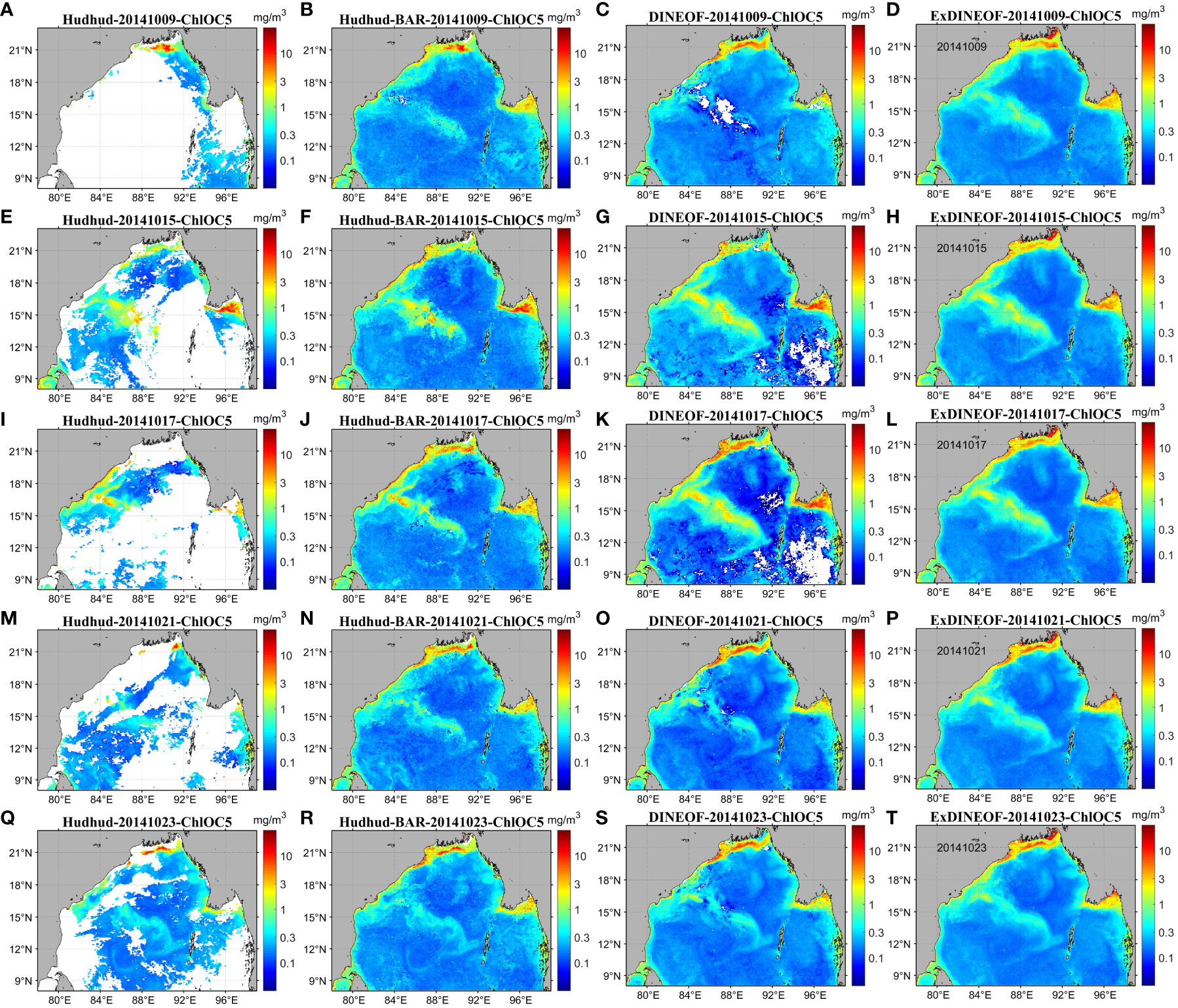
Figure 7 Spatial distribution of the original (A, E, I, M, Q) and reconstructed ChlOC5 data using the BAR (B, F, J, N, R), DINEOF (C, G, K, O, S), and ExDINEOF (D, H, L, P, T) methods.

By contrasting the reconstruction outcomes attained via various methods, as exhibited in Figure 7, it becomes evident that the ExDINEOF approach yielded the most comprehensive spatial distribution of reconstructed results, encompassing the most intricate temporal variations, and offering the most exhaustive local details. In summary, when compared with the commonly adopted univariate DINEOF and BAR methods, the ExDINEOF approach showed superior performance in terms of daily reconstruction for small-scale regions in relation to spatial distribution.

3.3 Accuracy assessment of the reconstructed results for chlorophyll-a concentration data for ExDINEOF and the alternative methods

3.3.1 Evaluation of the accuracy of randomly selected points via bootstrap-type analysis

In this study, a validation dataset comprising 200 randomly selected points per day (totaling 6200 data points) with valid data, yet without data reconstruction, was employed. These pre-selected points were subjected to one-to-one comparison with the reconstructed data points at corresponding locations. The findings demonstrated that the ExDINEOF method exhibited satisfactory accuracy, along with stability in correlation coefficients, residuals, and relative errors, thereby showing potential for application.

A prevalent technique for evaluating data reconstruction methods involves conducting a bootstrap-type analysis. This entails removing a portion of the original non-missing data before data reconstruction (with these data points not being involved in the reconstruction calculations). Subsequently, the removed original data is compared with the reconstructed data. In this study, the same methodology was adopted to validate the results of data reconstruction. Specifically, 200 pixels (corresponding to numbers 1001–1200 of the original data) were randomly chosen within the study area to assess the ExDINEOF method (as depicted in Figure 4). The outcomes of data reconstruction for a small spatial scale on a daily basis are presented in Figure 8.

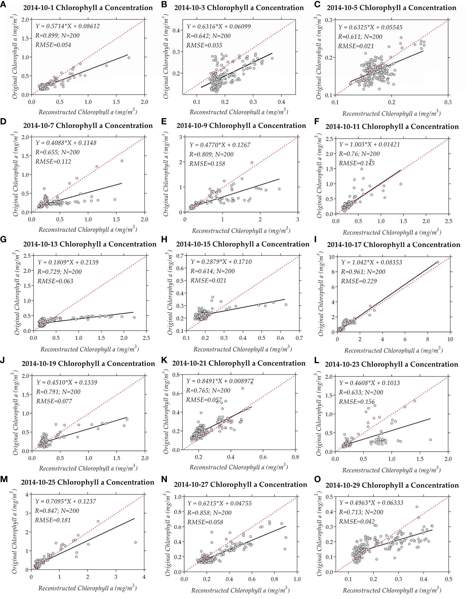
Figure 8 Bootstrap-type analysis of 200 data points for the reconstructed and original ChlOC5 chlorophyll-a concentration data in the study area using the ExDINEOF method. (A–O) show the daily comparison using the ExDINEOF method at an interval of 2 days from October 1–30, 2014.

The outcomes of data reconstruction were demonstrated for the 31-day time series of tropical cyclone Hudhud, encompassing its occurrences before, during, and after transit from October 1 to 31, 2014. In this process, the 200 sample points were preemptively removed to facilitate comparison. The time series correlation coefficients between the reconstructed and the original data are introduced in Figure 8, where the highest correlation coefficient exceeded 0.95 and the lowest correlation coefficient stood around 0.6. Among these coefficients, a certain level of variability was observed. The overall correlation coefficient between the original and ExDINEOF data for the 6200 data points was 0.859. Additionally, the data for residuals and relative errors exhibited robustness (Figure 9).

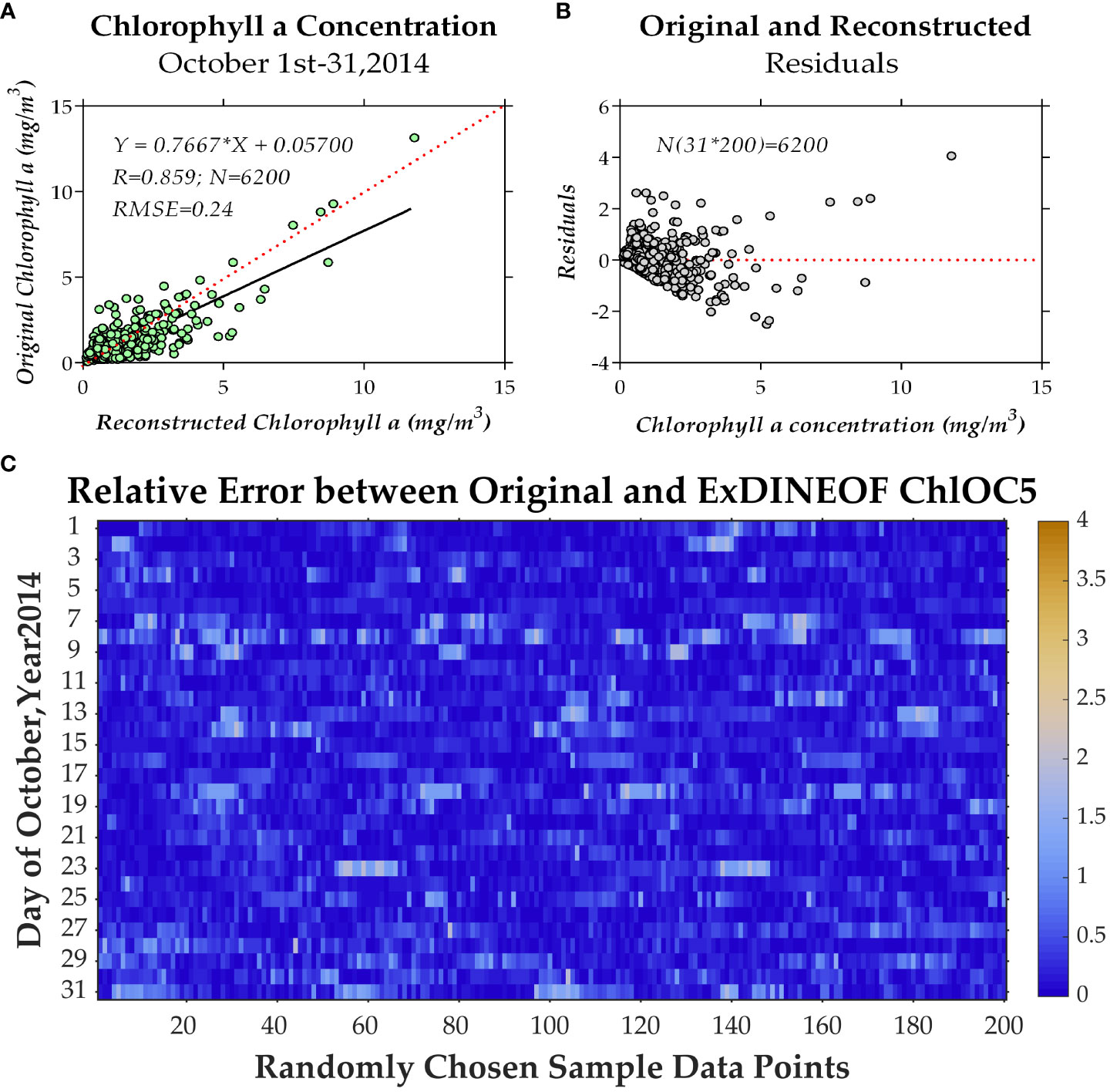
Figure 9 The overall correlation coefficients (A) and error distribution (B, C) for all 6200 data points.

3.3.2 Evaluation of accuracy of time series for selected spatial points

Conducting data reconstruction studies within the estuarine coastal zone, characterized by heightened dynamic forces in its water bodies compared to other regions, poses increased challenges. In this regard, the region delineated by the red dashed box in panel (a), situated at the mouth of the Ganges River in the northern Bay of Bengal, was singled out for time series assessment. A comparison of the absolute values and trends of the 30-day time series (outliers excluded) was carried out based on the regional mean.

The reconstructed values for the regional average preceding, during, and subsequent to the passage of tropical cyclone Hudhud over 30 consecutive days were selected to illustrate the phytoplankton’s biogenesis and extinction processes. Additionally, the 30-day time-series data reconstructed by the three methods were compared with the original satellite data to ascertain the method yielding the most accurate absolute results and trends in the time-series changes. Panel (b) of Figure 10 presents a comparison of the regional averages for the 30-day time series within the test area. The red dotted line in panel (b) signifies that the concentration values of chlorophyll-a within the phytoplankton in this region were low (around 4 mg/m³) from the start of October until approximately day 10. From October 12, the chlorophyll-a concentration values surged rapidly, peaking around October 23 (12 mg/m³), before swiftly declining to around 4 mg/m³. The complete journey of phytoplankton’s growth and subsequent extinction can be traced by examining the regional average values displayed in panel (b) spanning from day 1 to day 30.

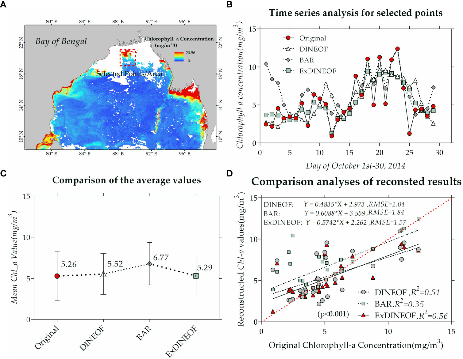
Figure 10 Comparison of time series for selected spatial regions (A). (B) Time series analysis of different reconstruct methods for selected region. (C) The comparison of region average values. (D) Comparison analyses of reconstructed results of different methods.

The original chlorophyll-a concentration data and the reconstructed remote sensing data (validated regional average) were compared in terms of trends, mean values, and correlation coefficients. In panel (b), the differences in absolute values of the reconstructed and original values for the 30-day time series within the region were compared. In the initial 5 days of October, the BAR reconstruction exhibited significant differences in both trend and absolute value due to the scarcity of sample data arising from the extensive missing data area. This disparity notably improved by mid-October, as the area of missing data diminished and sample size increased. Both DINEOF (triangular line) and ExDINEOF (rectangular line) closely aligned with the original satellite data in terms of overall trend, making it difficult to discern apparent distinctions between the two methods from panel (b). Panel (c) facilitates a comparison of the mean values for the study area (panel (a)), indicating that the mean values for ExDINEOF showed the least divergence from the original data, while the BAR reconstruction exhibited the largest error. A correlation analysis between the original and reconstructed data was carried out, with panel (d) illustrating that the correlation coefficient between the ExDINEOF data and the original data stood at 0.748, surpassing both DINEOF (R of 0.714) and BAR (R of 0.592).

Overall, the reconstructed data reflect the phytoplankton’s growth and extinction processes, with ExDINEOF yielding superior results for reconstructed outcomes, followed by DINEOF. Meanwhile, the BAR results proved the most variable, as they were heavily contingent upon the number of sample data available.

4 Discussion

4.1 Marine physical environmental factors associated with chlorophyll-a concentration

Overall, in Region B (depicted in Figure 1), traversed by cyclone Hudhud within the central-western expanse of the Bay of Bengal, the flow field’s velocity exhibited continuous augmentation, reaching its zenith during October 9–13 (Figures 11E–G). Notably, during intense winds, the sea surface height (SSH) in the region diminished to its nadir during October 9–13, subsequently showing a gradual ascent. The reconstructed chlorophyll-a concentration achieved its zenith during October 15–19 (Figures 5H–J), subsequently experiencing a decline. Moreover, a circular striped area with low SST was discernible in the region during October 9–15 (Figures 12E–I). The SSH and SST values exhibited an inverse relationship with the chlorophyll-a concentration. Specifically, lower SSH and SST values corresponded to higher chlorophyll-a concentration. However, a discernible time lag existed between SSH, SST, and chlorophyll-a concentration, with the maximal chlorophyll-a concentration occurring approximately 4–5 days subsequent to the nadir in SSH and SST values (Figure 13F).

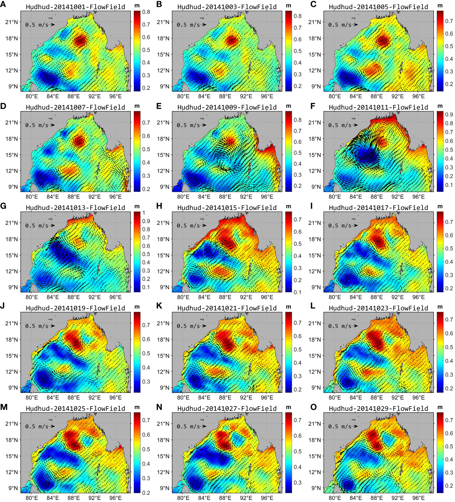
Figure 11 Daily reanalyzed SSH and flow field in the Bay of Bengal in October 2014. (A–O) show the daily reanalyzed SSH and the flow field at intervals of 2 days from October 1–30, 2014.

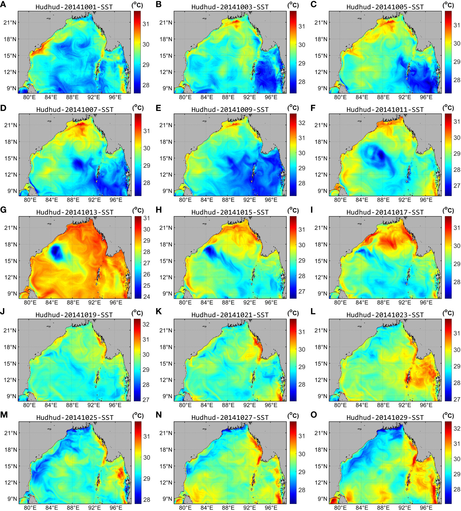
Figure 12 Daily reanalyzed SST in the Bay of Bengal in October 2014. (A–O) show the daily reanalyzed SST at an interval of 2 days from October 1–30, 2014.

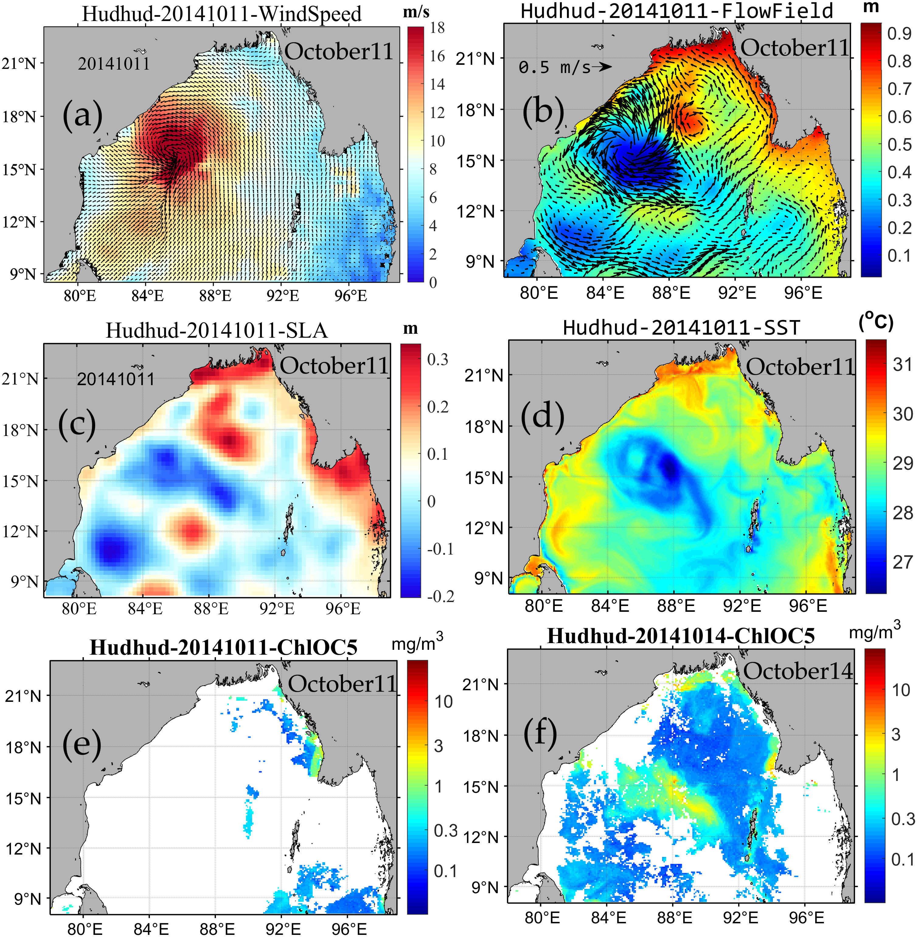
Figure 13 Relationship between chlorophyll a concentration (E, F) and environmental factors such as SST (D), Flow field (B), wind speed (A) and SSH (C).

It should be noted that both Region B and Region A (corresponding to the regions of Figure 1) displayed areas characterized by low SSH but high flow rates. However, Region A exhibited low chlorophyll-a concentration. As depicted in Figure 12, an anomalous region with considerably lower SST (approximately 3°C below surrounding areas) was evident in Region B, contrasting with Region A’s elevated SST values (Figure 13D).

In conclusion, a discernible correlation emerged between chlorophyll-a concentration and the variation of environmental factors. Specifically, anti-clockwise cyclonic winds (Figure 13A) induced anti-clockwise sea surface current rotation, culminating in an anti-clockwise vortex (Figure 13B). These forces dispersed surface waters into adjacent regions, consequently lowering sea surface height within the eddy zone compared to its surroundings (Figure 13C). This, in turn, triggered the upwelling of cooler nutrient-rich waters from the depths to the surface through Ekman Pumping, leading to lower sea surface temperatures than neighboring regions (Figure 13D).

Phytoplankton underwent distinct movements based on the sea layers. On the one hand, Ekman pumping led to the upwelling of subsurface phytoplankton into the sea surface layer. On the other hand, phytoplankton blossomed in the mixed layer post-upwelling of cold water. Adequate temperature, ample light, and nutrients from cold water beneath facilitated phytoplankton bloom, peaking 4-5 days after the severe tropical cyclone passage (Figures 13F, 5I, J). Subsequently, nutrient depletion reduced phytoplankton amounts (Figures 5M–O). Reflecting upon this and taking environmental elements into account, the ExDINEOF-based reconstructed chlorophyll-a concentrations excellently documented phytoplankton development pre, during, and post the severe tropical cyclone passage. These findings underscore the efficacy of employing the ExDINEOF technique for reconstructing daily-scale chlorophyll-a concentrations.

4.2 Analysis of the causes of differences in the accuracy of the time series

Figure 14 shows the spatial distribution of points (red data points within the red oval box) displaying correlation coefficients exceeding 0.8 (Figures 14A–L) and hovering around 0.6 (Figures 14M–R) between reconstructed and original data. As highlighted by Figure 14, the distribution of points with correlation coefficients exceeding 0.8 and around 0.6 lacks a discernible pattern. To probe into the reasons behind discrepancies between original satellite and ExDINEOF-reconstructed data, the relative error encompassing the entire Bay of Bengal was calculated.

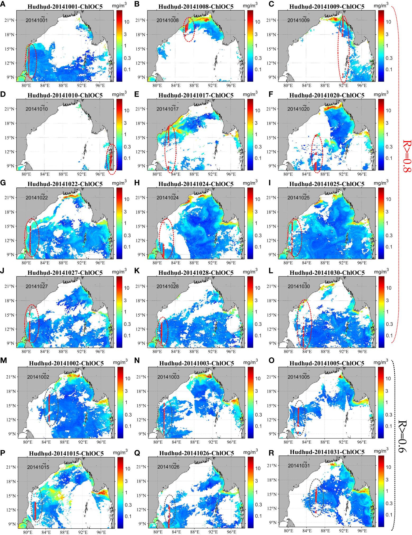
Figure 14 Spatial distribution of the points (red oval box) randomly selected by bootstrap-type analysis with correlation coefficients greater than 0.8 (A–L) and around 0.6 (M–R) between the original and reconstructed data.

To scrutinize the technical proficiency of ExDINEOF, an evaluation of the spatial distribution of relative errors was executed on several days following the severe tropical cyclone Hudhud’s transit. Data for October 16 and 18 pertained to phytoplankton blooms, while data for October 24 and 25 related to phytoplankton extinction.

Figure 15 displays the original satellite data in the left column (a, d, g, j), outcomes of ExDINEOF reconstruction in the middle column (b, e, h, k), and relative errors between the two in the right column (c, f, i, l). The spatial distribution of relative errors generally fell below 0.3 across most areas. Especially on October 25, when phytoplankton were diminishing, relative errors were mostly below 0.1. Notably, ExDINEOF didn’t manifest significantly higher relative errors in the nearshore area—typically marked by substantial errors and complex influencing factors. This highlights ExDINEOF’s applicability in nearshore regions characterized by high turbidity, dynamics, and complexity. Regions featuring substantial relative errors were predominantly situated near the phytoplankton blooms zone within the central Bay of Bengal.

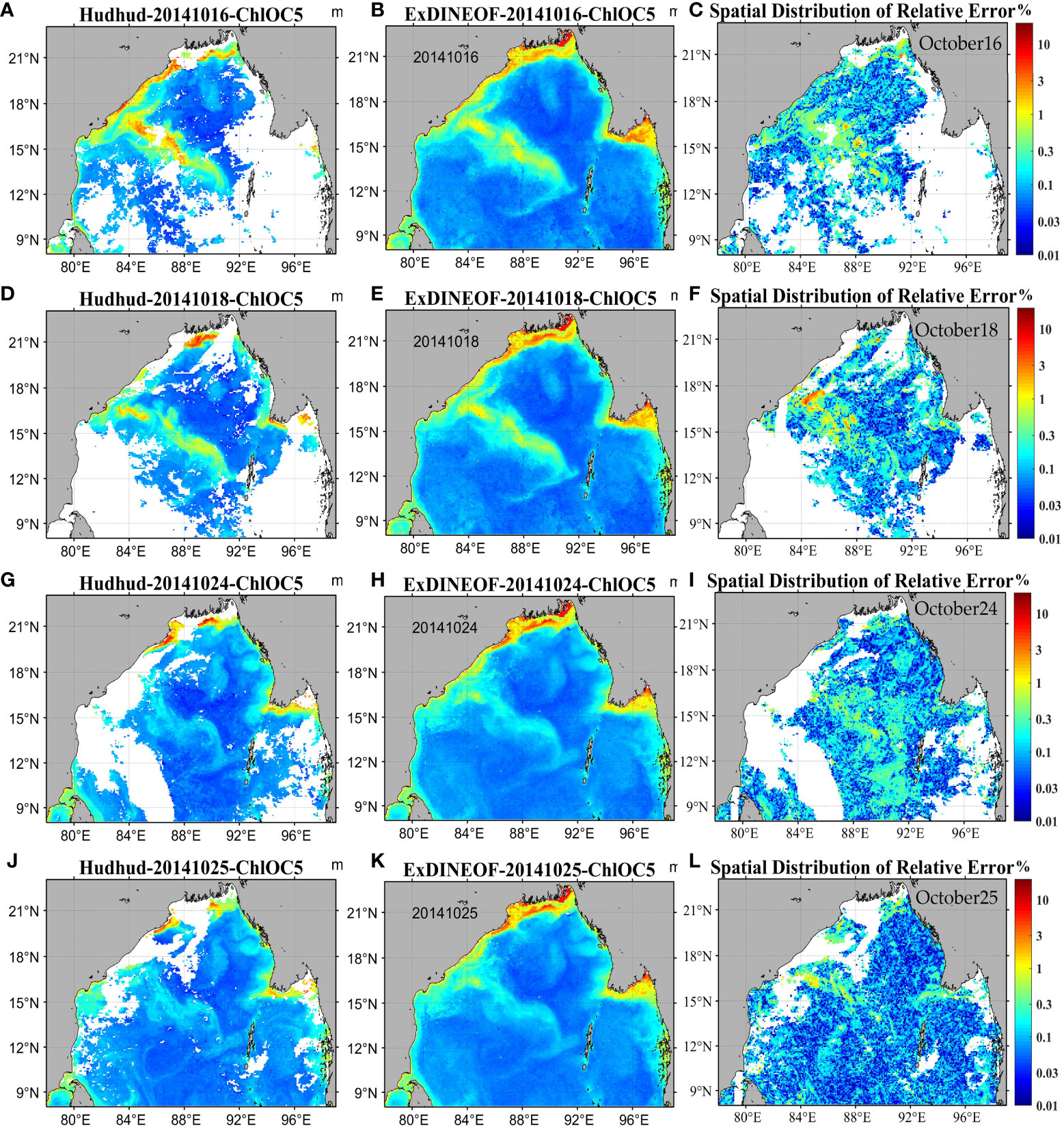
Figure 15 Spatial distribution of relative errors (C, F, I, L) in original (A, D, G, J) and ExDINEOF reconstructed data (B, E, H, K).

Instances of rapid phytoplankton blooms and extinctions are marked by their high-frequency characteristics in remote sensing data. The spatial distribution of the relative errors provides insight. Notably, ExDINEOF successfully reconstructs a significant portion of the high-frequency information, displaying reasonable spatial distribution and discernible texture features. However, certain aspects of high-frequency information remain filtered out due to the inherent low-pass filtering nature of DINEOF. Consequently, the relative errors exhibit greater magnitudes in areas where phytoplankton blooms and extinctions manifest prominently.

4.3 Differences between the DINEOF and ExDINEOF methods

ExDINEOF and DINEOF methods distinctly diverge in outcomes, suggesting distinct intrinsic mechanisms at play. The conventional DINEOF method hinges on an extensive time series of sample datasets to identify trends within data. This method then extracts key modes of these trends to define the overall spatio-temporal characteristics of the original dataset, thus excelling at recuperating trends within long-term data. However, DINEOF tends to filter out spatial information at small and medium scales, as well as high-frequency information, over short timespans, treating them as noise.

In contrast, ExDINEOF eschews dependence on extended sample information, reconstructing missing data based on inherent nonlinear correlations between various environmental factors and simultaneous chlorophyll-a concentrations. These correlations arise as both factors are simultaneously influenced by atmospheric and oceanic dynamical processes. ExDINEOF captures high- and low-frequency information adeptly, demonstrating heightened sensitivity to high-frequency information (i.e., day-scale, rapid non-long-term shifts). This renders ExDINEOF effective in reconstructing missing chlorophyll-a concentrations within dynamic, nearshore water bodies. This distinction likely underpins differences in time series accuracy.

Conventional DINEOF has some drawbacks: (1) It inherently performs low-pass filtering and smoothing within three-dimensional spatio-temporal data across time and space dimensions. A limited set of key modes characterizes the overall spatio-temporal traits, favoring long-term trend analysis. However, this method erases small-to-medium-scale spatial and temporal information as noise. (2) Randomly selected cross-validation data for DINEOF reconstruction can incorporate anomalous values, propagating errors if these data points are flawed. The selection of such data significantly influences subsequent error determination, optimal reconstruction mode, and the number of reconstructions. (3) To ensure reconstruction precision, pixels within time series covering less than a certain ratio (2%) must be preemptively removed, marking them as land areas. Failing to do so results in the reconstructed image becoming an average of the original, potentially leading to reconstruction failure. This issue historically prompted reconstructions on a monthly scale to ensure adequate data samples (Wang and Liu, 2014; Wang et al., 2019).

ExDINEOF supersedes original DINEOF due to: (1) Embracing the self-adaptive nature of original mono-variate DINEOF, negating the need for prior variable correlation values. (2) Recovery of the same variable’s correlations at different moments and of different variables at the same moment. (3) Utilization of spatial and temporal proximity to reconstruct missing data based on closely correlated factors’ signals. (4) Incorporating multiple data sources like thermal infrared remote sensing, optical remote sensing, microwave remote sensing, numerical modeling, and observations, all influenced differently by clouds and thus complementary (Figure 3).

5 Conclusion

This paper presents the adaptation and utilization of the ExDINEOF, a DINEOF-based data reconstruction method, for the purpose of reconstructing daily chlorophyll-a concentration data while considering various closely linked environmental factors. The ExDINEOF method, initially devised for small-scale daily reconstruction of SST data in the West Florida Shelf Alvera-Azcárate et al., 2007), was applied to reconstruct daily chlorophyll-a concentrations in the challenging context of a severe tropical cyclone passage over the Bay of Bengal, marked by limited data availability. The improved ExDINEOF proved valuable in reconstructing fine-grained daily chlorophyll-a concentrations during the transit of a severe tropical cyclone, with an emphasis on local spatial information. Comparative analysis was undertaken among the ExDINEOF method and similar data-reconstruction techniques, with a focus on the spatial distribution of the reconstructed outcomes. Furthermore, to gauge the absolute accuracy of the original satellite data and the reconstructed data, a bootstrap-type analysis was executed. This involved removing a portion of the initial data (specifically satellite chlorophyll-a measurements in this scenario) prior to the data reconstruction process. Subsequently, the removed original data were juxtaposed against the reconstructed data. Additionally, a time series comparison was performed for selected spatial points to further evaluate the performance of the ExDINEOF method.

The findings unequivocally demonstrate that the ExDINEOF method successfully recuperated the absent daily chlorophyll-a concentrations within the timeframe of a typical severe tropical cyclone. This was achieved with comprehensive and detailed spatial information at a local scale. Moreover, the method aptly captured the progression of phytoplankton growth, bloom, and extinction. In terms of spatial distribution of the reconstructed data, the ExDINEOF method showed superior results when contrasted with other prevalent data reconstruction methods. Evaluation of the accuracy for chlorophyll-a concentration data reconstruction confirmed that the ExDINEOF method surpassed the BAR method and the traditional mono-variate DINEOF method in terms of accuracy.

The ExDINEOF approach yielded satisfactory outcomes in reconstructing daily chlorophyll-a concentrations within the designated study area. These results serve as a valuable reference for future endeavors focused on reconstructing daily chlorophyll-a concentrations in similar small-to-medium regions. Additionally, they lend support to subsequent investigations concerning the impact of short-term, small-scale fluctuations in environmental factors on marine phytoplankton. Nevertheless, the methodology employed in this investigation carries certain limitations. First, the validation data points were constrained due to the abbreviated duration of the severe tropical cyclone. Second, the multitude of environmental factors influencing chlorophyll-a concentrations is intricate and diverse. As a consequence, not all these factors were incorporated into the reconstruction model. Looking ahead, with the advancement of numerical simulation technology in marine ecology, the challenge of reconstructing missing (daily) data can be tackled through the amalgamation of remote sensing and numerical modeling.

Data availability statement

The original contributions presented in the study are included in the article/supplementary material. Further inquiries can be directed to the corresponding author.

Author contributions

All authors contributed substantially to the design of this study, the analysis of the data, drafting the work, and interpreting result. ZW, PD, and QZ conceived and designed the framework of this research; ZW performed the experiments and wrote the paper; JD analyzed the data; SQ, and XD gave comments and suggestions to the manuscript; JL checked the writing and provided many helpful suggestions. All authors contributed to the article and approved the submitted version.

Funding

This research was funded by the Talent cultivation project of Henan Academy of Sciences(230501008); Central Guiding Locals Science and Technology Development Special Project (211201004); Science and Technology Research Project of Henan Province (222102320467, 232102321100); Major Scientific Research Focus Project of Henan Academy of Sciences (210101007); and the funding provided by the innovation team of quantitative remote sensing and intelligent analysis of ecological environment, Henan Academy of Sciences.

Acknowledgments

The authors would like to thank the reviewers and the editor for their constructive comments.

Conflict of interest

The authors declare that the research was conducted in the absence of any commercial or financial relationships that could be construed as a potential conflict of interest.

Publisher’s note

All claims expressed in this article are solely those of the authors and do not necessarily represent those of their affiliated organizations, or those of the publisher, the editors and the reviewers. Any product that may be evaluated in this article, or claim that may be made by its manufacturer, is not guaranteed or endorsed by the publisher.

References

Alvera-Azcárate A., Barth A., Beckers J. M., Weisberg R. H. (2007). Multivariate reconstruction of missing data in sea surface temperature, chlorophyll, and wind satellite fields. J. Geophys. Res. 112(C3). doi: 10.1029/2006JC003660
Alvera-Azcárate A., Barth A., Parard G., Beckers J. (2016). Analysis of SMOS sea surface salinity data using DINEOF. Remote Sens. Environ. 180, 137–145. doi: 10.1016/j.rse.2016.02.044
Alvera-Azcárate A., Barth A., Rixen M., Beckers J. M. (2005). Reconstruction of incomplete oceanographic data sets using empirical orthogonal functions: application to the Adriatic Sea surface temperature. Ocean Model. 9 (4), 325–346. doi: 10.1016/j.ocemod.2004.08.001
Alvera-Azcárate A., Barth A., Sirjacobs D., Beckers J. M. (2009). Enhancing temporal correlations in EOF expansions for the reconstruction of missing data using DINEOF. Ocean Sci. 5 (4), 475–485. doi: 10.5194/os-5-475-2009
Alvera-Azcárate A., Vanhellemont Q., Ruddick K., Barth A., Beckers J. (2015). Analysis of high frequency geostationary ocean colour data using DINEOF. Estuarine Coast. Shelf Sci. 159, 28–36. doi: 10.1016/j.ecss.2015.03.026
Antoine D., D'Ortenzio F., Hooker S. B., Becu G., Gentili, Tailliez B. D., et al. (2008). Assessment of uncertainty in the ocean reflectance determined by three satellite ocean color sensors (MERIS, SeaWiFS and MODIS-A) at an offshore site in the Mediterranean Sea (BOUSSOLE project). J. Geophys. Res. 113 (C7). doi: 10.1029/2007JC004472
Beckers J. M., Barth A., Alvera-Azcárate A. (2006). DINEOF reconstruction of clouded images including error maps - application to the Sea-Surface Temperature around Corsican Island. Ocean Sci. 2 (2), 183–199. doi: 10.5194/os-2-183-2006
Beckers J. M., Rixen M. (2003). EOF calculations and data filling from incomplete oceanographic datasets. J. Atmos. Oceanic Technol. 20 (12), 1839–1856. doi: 10.1175/1520-0426(2003)020<1839:ECADFF>2.0.CO;2
Bignami F., Sciarra R., Carniel S., Santoleri R. (2007). Variability of Adriatic Sea coastal turbid waters from SeaWiFS imagery. J. Geophys. Res. 112 (C3). doi: 10.1029/2006JC003518
Brando V. E., Braga F., Zaggia L., Giardino C., Bresciani M., Bellafiore D., et al. (2015). High-resolution satellite turbidity and sea surface temperature observations of river plume interactions during a significant flood event. Ocean Sci. 11 (6), 909–920. doi: 10.5194/os-11-909-2015
Bretherton F. P., Davis R. E., Fandry C. B. (1976). A technique for objective analysis and design of oceanographic experiments applied to MODE-73. Deep-Sea Res. Oceanogr. Abstracts 23 (7), 559–582. doi: 10.1016/0011-7471(76)90001-2
Chacko N. (2017). Chlorophyll bloom in response to tropical cyclone Hudhud in the Bay of Bengal: Bio-Argo subsurface observations. Deep Sea Res. Part I: Oceanogr. Res. Papers 124, 66–72. doi: 10.1016/j.dsr.2017.04.010
De Montera L., Jouini M., Verrier S., Thiria S., Crepon M. (2011). Multifractal analysis of oceanic chlorophyll maps remotely sensed from space. Ocean Sci. 7 (2), 219–229. doi: 10.5194/os-7-219-2011
Everson R., Cornillon P., Sirovich L., Webber A. (1996). An empirical eigenfunction analysis of sea surface temperatures in the Western North Atlantic. J. Phys. Oceanogr. 27 (3), 468–479. doi: 10.1063/1.50998
Gohin F., Druon J. N., Lampert L. (2010). A five channel chlorophyll concentration algorithm applied to SeaWiFS data processed by SeaDAS in coastal waters. Int. J. Remote Sens. 23 (8), 1639–1661. doi: 10.1080/01431160110071879
Grodsky S. A., Carton J. A. (2001). Intense surface currents in the tropical Pacific during 1996-1998. J. Geophys. Res. Atmos. 106 (C8), 16673–16684. doi: 10.1029/2000JC000481
Gunes H., Cekli H. E., Rist U. (2008). Data enhancement, smoothing, reconstruction and optimization by kriging interpolation, Simulation Conference. IEEE 2008 Winter Simulation Conference (WSC) - Miami, FL, USA (2008.12.7-2008.12.10), 379–386. doi: 10.1109/wsc.2008.4736091
Hilborn A., Costa M. (2018). Applications of DINEOF to satellite-derived chlorophyll-a from a productive coastal region. Remote Sens. 10 (9), 1449. doi: 10.3390/rs10091449
Iida T., Saitoh S. (2007). Temporal and spatial variability of chlorophyll concentrations in the Bering Sea using empirical orthogonal function (EOF) analysis of remote sensing data. Deep Sea Res. Part II: Topical Stud. Oceanogr. 54 (23-26), 2657–2671. doi: 10.1016/j.dsr2.2007.07.031
Jayaram C., Udaya Bhaskar T.V.S., Swain D., Rama Rao E.P., Bansal S., Dutta D., et al. (2014). Daily composite wind fields from Oceansat-2 scatterometer. Remote Sens. Lett. 5 (3), 258–267. doi: 10.1080/2150704X.2014.898191
Jayaram C., Priyadarshi N., Pavan Kumar J., Udaya Bhaskar T.V.S., Raju D., Kochuparampil A.J., et al. (2018). Analysis of gap-free chlorophyll-a data from MODIS in Arabian Sea, reconstructed using DINEOF. Int. J. Remote Sens. 39 (21), 7506–7522. doi: 10.1080/01431161.2018.1471540
Jayaram C., et al. (2021). Reconstruction of gap-free OCM-2 chlorophyll-a concentration using DINEOF. J. Indian Soc. Remote Sens. 49 (6), 1419–1425. doi: 10.1007/s12524-021-01317-6
Ji C., Zhang Y., Cheng Q., Tsou J., Jiang T., Liang X.S., et al. (2018). Evaluating the impact of sea surface temperature (SST) on spatial distribution of chlorophyll-a concentration in the East China Sea. Int. J. Appl. Earth Observ. Geoinform. 68, 252–261. doi: 10.1016/j.jag.2018.01.020
Jouini M., Lévy M., Crépon M., Thiria S. (2013). Reconstruction of satellite chlorophyll images under heavy cloud coverage using a neural classification method. Remote Sens. Environ. 131, 232–246. doi: 10.1016/j.rse.2012.11.025
Li Y., He R. (2014). Spatial and temporal variability of SST and ocean color in the Gulf of Maine based on cloud-free SST and chlorophyll reconstructions in 2003–2012. Remote Sens. Environ. 144, 98–108. doi: 10.1016/j.rse.2014.01.019
Liu X., Wang M. (2016). Analysis of ocean diurnal variations from the Korean Geostationary Ocean Color Imager measurements using the DINEOF method. Estuarine Coast. Shelf Sci. 180, 230–241. doi: 10.1016/j.ecss.2016.07.006
Liu X., Wang M. (2018). Gap filling of missing data for VIIRS global ocean color products using the DINEOF method. IEEE Trans. Geosci. Remote Sens. 56 (8), 4464–4476. doi: 10.1109/TGRS.2018.2820423
Liu X., Wang M. (2019). Filling the gaps of missing data in the merged VIIRS SNPP/NOAA-20 ocean color product using the DINEOF method. Remote Sens. 11 (2), 178. doi: 10.3390/rs11020178
Ma C., Zhao J., Ai B., Sun S. (2021). Two-decade variability of sea surface temperature and chlorophyll-a in the Northern South China Sea as revealed by reconstructed cloud-free satellite data. IEEE Trans. Geosci. Remote Sens. 59, 9033–9046. doi: 10.1109/TGRS.2021.3051025
Maeda E. E., Lisboa F., Kaikkonen L., Kallio K., Koponen S., and Brotas V., et al. (2019). Temporal patterns of phytoplankton phenology across high latitude lakes unveiled by long-term time series of satellite data. Remote Sens. Environ. 221, 609–620. doi: 10.1016/j.rse.2018.12.006
Martinez E., Gorgues T., Lengaigne M., Fontana C., Sauzéde R., and Menkes C., et al. (2020). Reconstructing global chlorophyll-a variations using a non-linear statistical approach. Front. Mar. Sci. 7. doi: 10.3389/fmars.2020.00464
NeChad B., Alvera-Azcaràte A., Ruddick K., Greenwood N. (2011). Reconstruction of MODIS total suspended matter time series maps by DINEOF and validation with autonomous platform data. Ocean Dynamics 61 (8), 1205–1214. doi: 10.1007/s10236-011-0425-4
Novelli A., Tarantino E., Fratino U., Iacobellis V., Romano G., Gentile F. (2016). A data fusion algorithm based on the Kalman filter to estimate leaf area index evolution in durum wheat by using field measurements and MODIS surface reflectance data. Remote Sens. Lett. 7 (5), 476–484. doi: 10.1080/2150704X.2016.1154219
Park K. A., Chae H. J., Park J. E. (2013). Characteristics of satellite chlorophyll-a concentration speckles and a removal method in a composite process in the East/Japan Sea. Int. J. Remote Sens. 34 (13), 4610–4635. doi: 10.1080/01431161.2013.779397
Ping B., Su F., Meng Y., Coles J. A. (2016). An improved DINEOF algorithm for filling missing values in spatio-temporal sea surface temperature data. PloS One 11 (5), e0155928–e0155928. doi: 10.1371/journal.pone.0155928
Pottier C., Turiel A., Garçon V. (2008). Inferring missing data in satellite chlorophyll maps using turbulent cascading. Remote Sens. Environ. 112 (12), 4242–4260. doi: 10.1016/j.rse.2008.07.010
Reynolds R. W., Smith T. M. (1994). Improved global sea surface temperature analyses using optimum interpolation. J. Climate 7 (6), 929–948. doi: 10.1175/1520-0442(1994)007<0929:IGSSTA>2.0.CO;2
Roxy M. K., Ritika K., Terray P., Masson S. (2014). The curious case of Indian Ocean warming. J. Climate 27 (22), 8501–8509. doi: 10.1175/JCLI-D-14-00471.1
Shropshire T., Li Y., He R. (2016). Storm impact on sea surface temperature and chlorophyll-a in the gulf of mexico and sargasso sea based on daily cloud‐free satellite data reconstructions. Geophys. Res. Lett. 43 (23). doi: 10.1002/2016GL071178
Sirjacobs D., Alvera-Azcarate A., Barth A., Lacroix G., Park Y., and Nechad B., et al. (2011). Cloud filling of ocean colour and sea surface temperature remote sensing products over the Southern North Sea by the Data Interpolating Empirical Orthogonal Functions methodology. J. Sea Res. 65 (1), 114–130. doi: 10.1016/j.seares.2010.08.002
Sravanthi N., Ali P. Y., Narayana A. C. (2017). Merging gauge data and models with satellite data from multiple sources to aid the understanding of long-term trends in chlorophyll-a concentrations. Remote Sens. Lett. 8 (5), 419–428. doi: 10.1080/2150704X.2016.1278308
Thompson B., Tkalich P., Malanotte-Rizzoli P. (2017). Regime shift of the South China Sea SST in the late 1990s. Climate Dynamics 48 (5-6), 1873–1882. doi: 10.1007/s00382-016-3178-4
Waite J. N., Mueter F. J. (2013). Spatial and temporal variability of chlorophyll- a concentrations in the coastal Gulf of Alaska 1998–2011, using cloud-free reconstructions of SeaWiFS and MODIS-Aqua data. Prog. Oceanogr. 116 (9), 179–192. doi: 10.1016/j.pocean.2013.07.006
Wang Z., Du J., Xia J., Chen C., Zeng Q., Tian L., et al. (2020). An effective method for detecting clouds in GaoFen-4 images of coastal zones. Remote Sens. 12 (18), 3003. doi: 10.3390/rs12183003
Wang Y., Gao Z., Liu D. (2019). Multivariate DINEOF reconstruction for creating long-term cloud-free chlorophyll-a data records from SeaWiFS and MODIS: A case study in Bohai and Yellow Seas, China. IEEE J. Select. Topics Appl. Earth Observ. Remote Sens. 12 (5), 1383–1395. doi: 10.1109/JSTARS.2019.2908182
Wang Y., Liu D. (2014). Reconstruction of satellite chlorophyll-a data using a modified DINEOF method: a case study in the Bohai and Yellow Seas, China. Int. J. Remote Sens. 35 (1), 204–217. doi: 10.1080/01431161.2013.866290
Xiao C., Chen N., Hu C., Wang K., Xu Z., Cai Y., et al. (2019). A spatiotemporal deep learning model for sea surface temperature field prediction using time-series satellite data. Environ. Model. Softw. 120, 104502. doi: 10.1016/j.envsoft.2019.104502
Xiu P., Liu Y., Rong Z., Zong H., Li G., Xing X., et al. (2007). Comparison of chlorophyll algorithms in the Bohai Sea of China. Ocean Sci. J. 42 (4), 199–209. doi: 10.1007/BF03020911
Yu Y., Xing X., Liu H., Yuan Y., Wang Y., Chai F., et al. (2019). The variability of chlorophyll-a and its relationship with dynamic factors in the basin of the South China Sea. J. Mar. Syst. 200, 103230. doi: 10.1016/j.jmarsys.2019.103230
Zhang Y., Rabbani M., Stevenson R.L., Zhao D., Ma S., Wang R., et al. (2009). A 3D auto-regressive model for bidirectional prediction. Int. Soc. Optics Photonics 7257, 72571I. doi: 10.1117/12.805698
Keywords: data reconstruction, chlorophyll-a concentration, ExDINEOF, Bay of Bengal, severe tropical cyclone, Hudhud
Citation: Wang Z, Qiu S, Zeng Q, Du P, Dang X, Liu J and Du J (2023) Reconstruction of daily chlorophyll-a concentrations in the transit of severe tropical cyclone Hudhud using the ExDINEOF method. Front. Mar. Sci. 10:1230116. doi: 10.3389/fmars.2023.1230116
Received: 29 May 2023; Accepted: 28 August 2023;
Published: 18 September 2023.
Edited by:
Sudheer Joseph, Indian National Centre for Ocean Information Services, IndiaReviewed by:
Ana B. Ruescas, University of Valencia, SpainAlakes Samanta, Indian National Centre for Ocean Information Services, India
Copyright © 2023 Wang, Qiu, Zeng, Du, Dang, Liu and Du. This is an open-access article distributed under the terms of the Creative Commons Attribution License (CC BY). The use, distribution or reproduction in other forums is permitted, provided the original author(s) and the copyright owner(s) are credited and that the original publication in this journal is cited, in accordance with accepted academic practice. No use, distribution or reproduction is permitted which does not comply with these terms.
*Correspondence: Jun Du, dujun@igs-has.cn