Long-term over-the-horizon microwave channel measurements and statistical analysis in evaporation ducts over the Yellow Sea

1 Introduction

With a rapid expansion of maritime economy, such as transportation, oil exploitation, fishery, tourism and environment monitoring, the demand for new maritime broadband long-range communication technology has increased dramatically in recent years. Evaporation ducts are formed in the atmospheric surface layer owing to seawater evaporation. Behaving like a waveguide, evaporation ducts can have dramatic impact on microwave instruments, especially those operating in the C- and X-bands (Hitney and Hitney, 1990; Shi et al., 2019). Evaporation ducts can lead to diminished attenuation of the signal, which can be utilized to achieve long-range maritime broadband communication. Evaporation ducts have been used to establish a number of over-the-horizon maritime broadband microwave links (Woods et al., 2009; Couillard et al., 2018; Zaidi et al., 2021; Ma et al., 2022; Yang et al., 2022b).

However, the findings of those communication tests have rarely been utilized in engineering applications. The main reason is that duct environments are volatile, uncontrollable, and severely affected by meteorological conditions, which makes over-the-horizon communication unreliable and difficult to predict. Therefore, detailed measurement, analysis, and modeling of duct channels are essential for application of reliable over-the-horizon maritime broadband communication. Over recent decades, the effects of different factors on EM wave propagation in evaporation ducts have been studied. The Rough Evaporation Duct experiment (Anderson et al., 2004) was conducted to study the effects of ocean waves on microwave propagation. Shi et al. (2015a) studied the effect of the horizontal inhomogeneity of evaporation ducts on EM wave propagation through an experiment conducted in the northern part of the South China Sea in December 2013. Shi et al. (2015b) investigated the influence of obstacles on EM wave propagation in an evaporation duct, and the experimental results showed that the presence of an island could cause increase of approximately 30–40 dB in PL. Shi et al. (2019) presented the frequency response of an evaporation duct channel measured in the South China Sea along a 149-km-long propagation path in 2014. Wang et al. (2020) studied the influence of antenna height on microwave propagation in an evaporation duct. Wang et al. (2022a) reported observations of anomalous over-the-horizon EM propagation of a 53-km-long link in evaporation ducts induced by typhoon Kompasu (202118). Yang et al. (2022c) reported the effects of rainfall on over-the-horizon EM propagation in evaporation ducts over the South China Sea.

Moreover, the long-term channel characteristics of the evaporation duct are also essential for the application of reliable and controllable over-the-horizon maritime broadband communication. A large number of long-term channel measurements have been conducted of EM propagation in evaporation ducts. The Tropical Air–Sea Propagation Study (Kulessa et al., 2017), which was conducted from November 24 to December 5, 2013, evaluated the ability to forecast EM propagation and provided researchers with a dataset for clear-air tropical littoral conditions around Australia’s Great Barrier Reef. The SoCal 2013 experiment (Pozderac et al., 2018), conducted off the coast of San Diego (CA, USA) during November 9–22, 2013, used an X-band beacon-receiver array system to record propagation loss for inversion of EDH. The Coupled Air–Sea Processes and Electromagnetic Ducting Research project (Wang et al., 2018; Wang et al., 2019; Ulate et al., 2019; Xu et al., 2022) was conducted to improve capability in characterizing the propagation of radio frequency signals through the marine duct environments, using platforms that included regional research vessels, research aircraft, buoys, radars, wave gliders, towers, tethered balloons, and X-band vertical array systems. The Coastal Land–Air–Sea Interaction project (Haus et al., 2022) incorporates EM propagation measurements using a coherent array, drone receiver, and a marine radar to study evaporation duct distributions in the coastal zone. On the basis of simulation and experiment, Robinson et al. (2022) analyzed the effects of evaporation ducts on microwave communications in the Irish Sea, and found that evaporation ducts could be used to provide high-bandwidth over-the-horizon communication with uptime of approximately 40%. Zhang et al. (2022) presented the measurement results of evaporation duct channel at 8 GHz in the South China Sea region.

The temporal and spatial distribution characteristics of evaporation duct show strong differences in different sea areas (Shi et al., 2015b; Sirkova, 2015; Yang et al., 2016; Zhang et al., 2016; Yang et al., 2022a; Huang et al., 2022). Lying between mainland China and the Korean Peninsula, the Yellow Sea is one of the largest areas of continental shelf shallow water that provides rich fishing grounds and oil resources. The channel characteristics of evaporation duct over the Yellow Sea has been seldom reported. This paper presents long-term measurements of over-the-horizon microwave propagation in evaporation ducts over the Yellow Sea in 2021. The X-band EM propagation systems, deployed in coastal areas of the Yellow Sea, recorded valid EM propagation data of a 133-km-long (7.7 times the line-of-sight length) link over a 54-day period in autumn. The EM propagation characteristics were analyzed on the basis of statistical analysis and model simulations. The results are important with regard to the development and application of over-the-horizon maritime broadband communication. The remainder of this paper is structured as follows. Section 2 presents details of the measurement campaign and outlines the methods used to study the effects of evaporation ducts on EM propagation. In Section 3, the measured data and their statistical properties are analyzed. Evaporation duct climatology during the measurement period and the effects of evaporation ducts on EM propagation based on model simulation are also presented in Section 3. The annual variation of evaporation ducts and the monthly average EDH distributions in the Yellow Sea are discussed in Section 4. Finally, the derived conclusions are presented in Section 5.

2 Data and method

This section presents basic information on the long-term measurements over the Yellow Sea during autumn 2021. The European Centre for Medium-Range Weather Forecasts (ECMWF) ERA5 reanalysis data and the Naval Atmospheric Vertical Surface Layer Model (NAVSLaM) were used to calculate the EDH distributions during the measurements. Then, the EM propagation model was used to study the effect of evaporation ducts on over-the-horizon EM wave propagation.

2.1 Measurement campaign

A long-term over-the-horizon microwave propagation link was established over the Yellow Sea for a 54-day period. The measurements were carried out from September 20 to November 22, 2021, with interruption during October 1–10 when the system was off. The measurement location is presented in Figure 1A. We have specially developed X-band EM propagation systems that can operate all day long to automatically record data of propagation characteristics. The PL data and meteorological parameters such as wind speed (WS), air temperature (AT), relative humidity (RH), and air pressure (AP) were recorded. For the measured data used in the current study, the receiver (Rx) was deployed in Rizhao City (S1), Shandong Province, and the transmitter (Tx) was deployed in Yancheng City (S2), Jiangsu Province. The length of the propagation link was approximately 133 km. For the antenna heights in this measurement, the line-of-sight horizon was $D=4.12\times \left(\sqrt{h_t}+\sqrt{h_r}\right)=4.12\times \left(\sqrt{6}+\sqrt{3}\right)=$ 17.2 km in a standard atmosphere, where h_t is the Tx height, and h_r is the Rx height. The link length was approximately 7.7 times the line-of-sight length. As shown Figure 1A, the P1, P2, P3, and P4 are the reanalysis meteorological data grid points along the propagation link, which were used for simulation analysis.

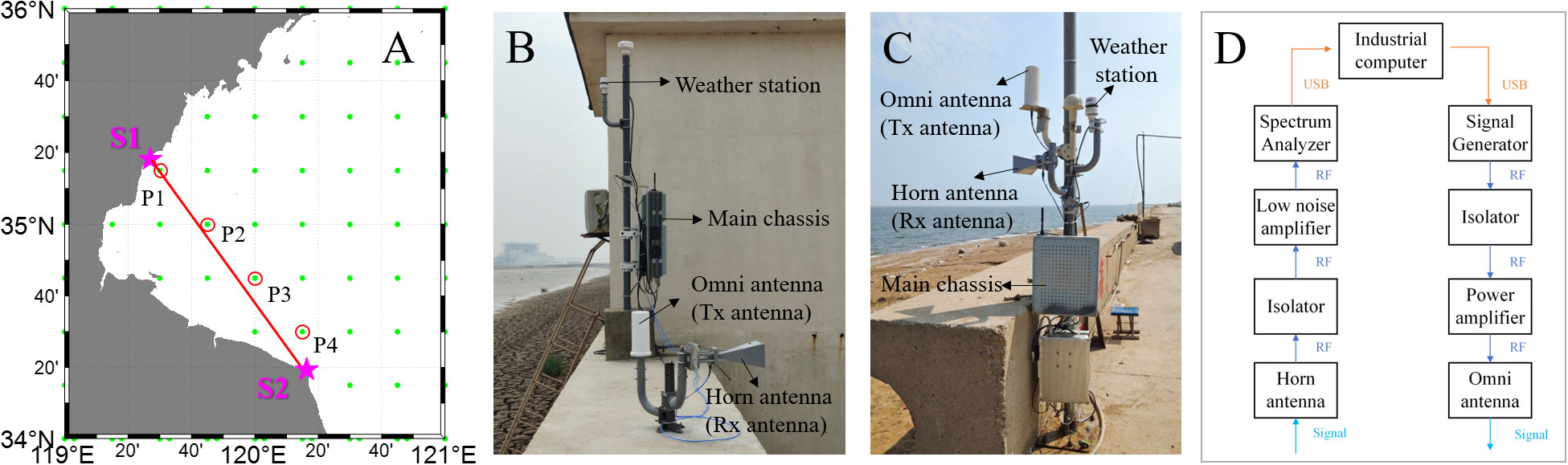
Figure 1 (A) Propagation path (red line), the positions of the transmitter and receiver (pink pentagrams) and reanalysis data grid points (green points and red circles), (B) transmitter (S2), (C) receiver (S1), (D) measurement system schematic.

Highly integrated and automated design enable the propagation system to operate for a long time in the marine environment. Photographs of the EM propagation systems are shown in Figures 1B, C. Figure 1D shows a schematic of this system. The EM propagation system is a combination of transceivers, and differentiates itself from other systems by setting different signal frequencies. The Tx includes a signal generator connected through an isolator to a power amplifier, and then to an omni antenna. The Rx includes a horn antenna connected through an isolator to a low noise amplifier, and then to a spectrum analyzer. The system configurations are shown in Table 1.

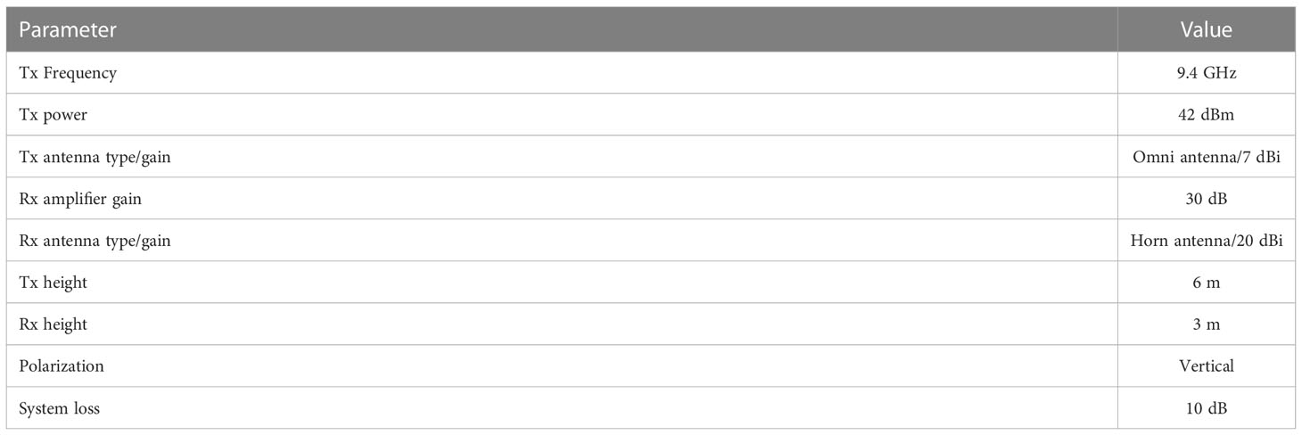
Table 1 Experimental configuration.

The industrial computer inside is used for sending the configuration instructions to the signal generator and collecting the data from the spectrometer. The received signal level (RSL) was recorded at approximately 1-s intervals using the internal computer. The RSL was mainly influenced by three aspects. 1) The change of the duct environment during the measurement; 2) the fading caused by the multipath effect in the duct; 3) the fading caused by passing ships along the propagation path due to the low height of the transmission channel. In addition, the received signal also includes noise when the over-the-horizon propagation cannot be realized due to poor duct environments. The existing measurement data can’t well deduce the small-scale fading channel properties. In order to statistically analyze the connectable probability of this over-the-horizon link, and to provide reference for other electromagnetic systems, the PL (dB) was converted from the RSL (Yang et al., 2022b) using the system parameters shown in Table 1 and the following equation:

where P_t is the Tx power (42 dBm), G_t is the Tx antenna gain (7 dBi), G_r is the Rx antenna gain (20 dBi), P_r is the Rx amplifier gain (30 dB), SL is the system loss (10 dB), and RSL (dB) is the received signal level.

2.2 Reanalysis data

Reanalysis data were used to determine the variations of the meteorological parameters and to simulate the long-term inhomogeneous evaporation duct environments for the analysis of over-the-horizon EM propagation. This study used ECMWF ERA5 data (Hersbach et al., 2020, 5), which is the fifth generation of the ECMWF global climate and weather product with temporal coverage extending from 1979 to the present. The temporal resolution of the ERA5 dataset is 1 h and the horizontal resolution is 0.25° × 0.25°. ERA5 data have been widely used and verified suitable for studies on evaporation duct distributions (Sirkova, 2015; Huang et al., 2022; Wang et al., 2022a; Wang et al., 2022b). The parameters of AT at 2-m height, AP, WS at 10-m height, RH at 1000 hPa, and sea surface temperature (SST) were extracted to simulate the EDH distributions during the measurements. The data on P1, P2, P3, and P4 shown in Figure 1A were used for the EDHs simulation along the propagation link.

2.3 Evaporation duct model

A long-range propagation mechanism is usually encountered at microwave frequencies owing to the trapping effect of ocean evaporation ducts. The propagation of EM radiation in the atmosphere depends upon the refractive index of air n, which varies in the troposphere due to the variation of pressure, temperature and water vapor content. The refraction index n is an electrical property of the propagation medium and is defined as the ratio between the speed of light in a vacuum, c₀, and the speed of the wave through the medium, v. For radio waves the refractive index of the troposphere is given based on Debye theory (Debye, 1929):

where T (K) represents air temperature, P (hPa) represents the total atmospheric pressure, and e (hPa) represents the partial pressure of water vapor (Smith and Weintraub, 1953). The partial pressure of water vapor e may be derived from the specific humidity using the equation:

where q (kg/kg) represents the specific humidity, and ϵ is the ratio of the individual gas constant for dry air to that for water vapor.

In the troposphere, the refractive index varies between 1.000250 and 1.000400 n-units. Because it is so close to unity, the refractive index of the troposphere is represented by a quantity called radio refractivity N, which is given by:

Under ducting conditions, EM propagation is refracted toward the earth’s surface so that it becomes trapped in a layer. To determine these conditions, the quantity modified refractivity M which takes into account the curvature of the earth’s surface, is often used. The modified refractivity M is defined by:

Where r_e (m) is the earth’s radius and z (m) is the altitude. In the regions with a negative vertical slope of M, EM propagation is refracted toward the surface and may become trapped in a leaky atmospheric duct.

The evaporation duct exists primarily due to a significant negative vertical gradient in humidity near the sea surface. In the evaporation duct layer, the M decreases as the sea surface height increases. When a certain height is reached, the M reaches a minimum value, and then increases with height. The height corresponding to the minimum point is defined as the EDH.

In this study, an evaporation duct model was used to calculate the evaporation duct distributions using ERA5 reanalysis data covering the measurement period. Many evaporation duct models based on Monin–Obukhov Similarity Theory, including the Paulus–Jeske model (Paulus, 1985), Musson–Gauthier–Bruth model (Musson-Genon et al., 1992), Liu–Katsaros–Businger model (Babin and Dockery, 2002), Babin–Young–Carton model (Babin, 1996), and NAVSLaM (Frederickson et al., 2000, 2), have been developed to obtain M-profiles. NAVSLaM has been verified against radiosonde measurements (Anderson et al., 2004; Pozderac et al., 2018; Wang et al., 2018; Wang et al., 2019), and is considered ideal for estimating EDH (Babin and Dockery, 2002). This study used NAVSLaM to diagnose the evaporation duct distributions.

As equation (3) and (4) shows, the pressure, temperature and partial pressure of water vapor profiles are needed to calculate the M-profiles. The NAVSLaM model derive these profiles from the following equations:

where T(z) and q(z) are the temperature and specific humidity at a given altitude z above the sea surface. z_0θ and z_0q represent integration constants called the temperature and specific humidity roughness length, respectively. θ_* and q_* are the Monin-Obukhov temperature and specific humidity scaling parameters, respectively. The values of z_0θ , z_0q , θ_* and q_* are calculated using the TOGA COARE 3.0 bulk flux algorithm (Fairall et al., 2003). κ is von Karman’s constant. Γ_d is adiabatic lapse rate. L is the Obukhov length. ψ_h  denotes the temperature function. g , R , correspond to gravity acceleration, and gas constant, respectively. T_v  is the mean value of virtual temperature at height of z₁ and z₂ .

The processed ERA5 data were input into NAVSLaM, and then the distributions of evaporation ducts during the measurement period were obtained.

2.4 Path loss model

For free space microwave propagation, PL can be expressed by the free-space loss using the following equation:

where PL_FSL is the free-space PL (dB), f is the signal frequency (MHz), and d is the propagation distance (km).

For the marine environment, reflection from the sea surface cannot be ignored, and PL can be modeled using the 2-Ray model. The reflection coefficient for a vertically polarized wave approaches -1, and the 2-ray PL model can be simplified (Lee et al., 2014) as follows:

where PL_2−ray is the 2-Ray PL (dB), λ is the wavelength (m), D is the propagation distance (m), h_t is the Tx height (m), and h_r is the Rx height (m).

Long-range propagation of microwaves over the sea is greatly affected by the duct-trapping mechanism. The parabolic equation (PE) method has been widely used to predict EM propagation in the troposphere. The standard PE can be obtained from the Helmholtz equation:

where u is a scalar component of the electric field, z is the height, x is the range, k₀ is the free-space wave number, and M is the modified refractivity. Parameter u is given by the Fourier split-step solution of PE as follows:

where F[▪]  and F⁻¹[▪] are the Fourier transform and the Fourier inverse transform, respectively, p is the transform variable, and δx is the range increment. More detailed information on the Fourier split-step PE solution can be found in Goldhirsh and Dockery (1998). The PL expressed by the PE field function u (PL_PE ) can be calculated as follows:

Numerous models based on the PE method have been developed, e.g., the Terrain Parabolic Equation Model (Barrios, 1994), Parabolic Equation Toolbox (Ozgun et al., 2020), and Advanced Propagation Model (APM) (Barrios et al., 2002). The APM is applied in the Advanced Refractivity Effects Prediction System, which is widely used in assessment of EM instruments. Moreover, the APM has been widely used and tested in different duct environments (Barrios et al., 2002; Shi et al., 2015a; Shi et al., 2015c). In this study, we used the APM to simulate the effects of evaporation duct inhomogeneity on EM propagation.

3 Analysis of measurements

This section presents the measured data that include the PL data of the 133-km link and the atmosphere parameters. Statistical analysis of PL is conducted, and duct climatology during the measurement period is analyzed on the basis of ERA5 data and the evaporation duct model. Then, evaluation of the duct effect on the propagation link, as simulated by the APM, is undertaken. Finally, an example analysis is presented to explore the reasons for the observed characteristics of over-the-horizon EM propagation in the Yellow Sea in autumn.

3.1 Measured data

The EM propagation systems and automatic weather stations were deployed in the coastal areas of the Yellow Sea. These systems acquired continuous data both of the PL of the 133-km over-the-horizon link at the frequency of 9.4 GHz, and of the atmosphere parameters of AP, RH, WS, and AT. Figure 2 shows the measured PL (788,806 points) during autumn 2021. It can be seen that the PL data fluctuated greatly with even 60 dB decrease from 205 dB to 145 dB, and exhibited strong diurnal variation. Owing to the limitation of the maximum power loss that can be measured with our measurement equipment, PL below the noise floor could not be monitored. As shown in Figure 2, for the 133-km link (7.7 times the line-of-sight length), over-the-horizon propagation often occurred in different duct environments. This shows potential for application to long-range maritime broadband communication systems. Detailed statistical analysis of the PL is presented in the next section. A typical example of over-the-horizon propagation, as shown in the orange box in Figure 2, will be analyzed in the section 3.5 to reveal the reasons for the drastic PL fluctuation of the channel.

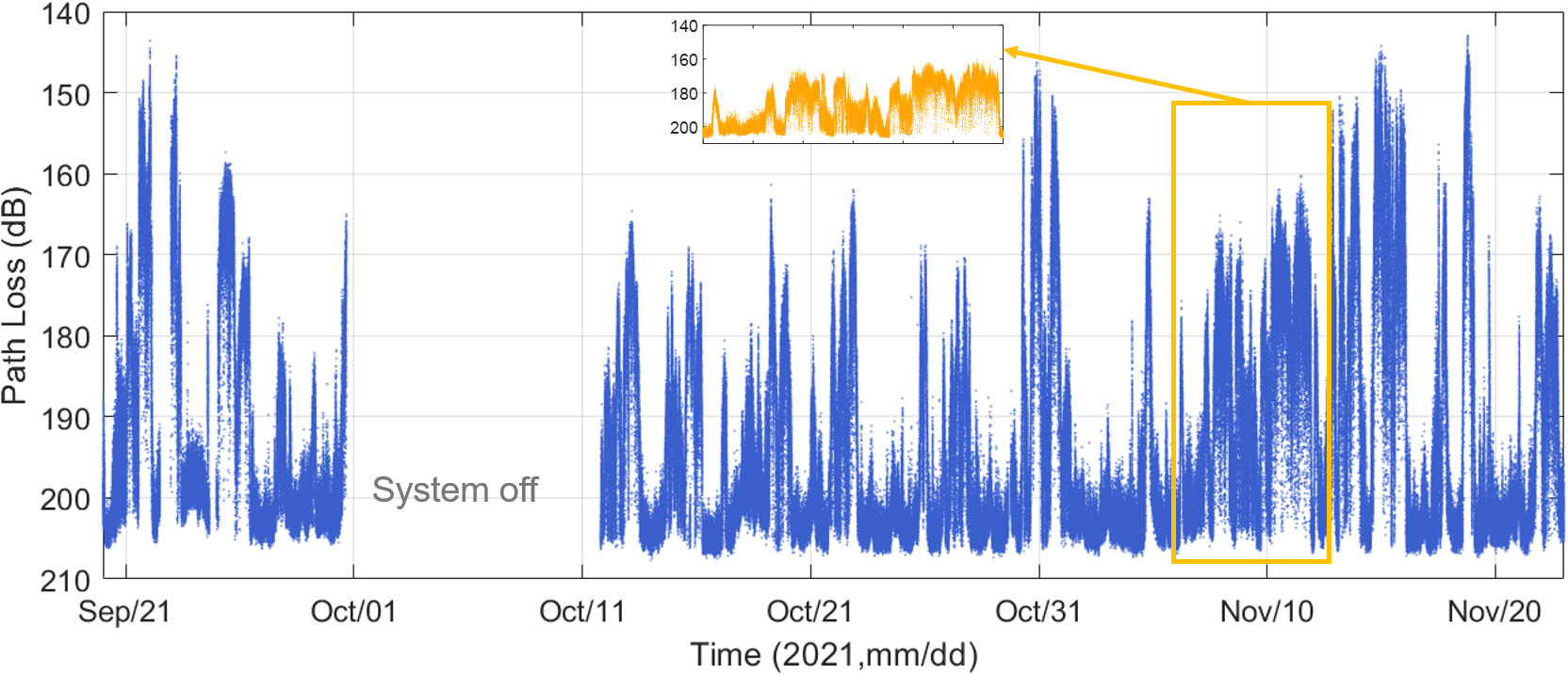
Figure 2 Observed PL data of the 133-km link over the Yellow Sea from September 20 to November 22, 2021.

Figure 3 shows the temporal evolutions of AP, RH, WS, and AT measured by the automatic weather stations installed at S1 and S2. It can be seen that the atmospheric parameters also fluctuated greatly with time. As shown in Figure 3A, the monitored AP was broadly similar at both locations. The RH and AT showed strong diurnal variation characteristics, as shown in Figures 3B, C, respectively. The RH varied greatly with values as low as 23% and as high as 98%. Generally, RH was low during the day and high at night, which might be attributable mainly to the light. The AT also exhibited strong diurnal variation with high temperatures during the day and low temperatures at night. The mean values of the measured AT were 23.3, 16.2, and 11.5 °C during September, October, and November, respectively, showing a general trend of decrease toward winter. As shown in Figure 3D, WS also varied greatly with values as low as 0 m/s and as high as 20 m/s, which would have marked influence on the evaporation of seawater. Overall, a large number of measured data were recorded, and both the PL and the meteorological parameters varied substantially.

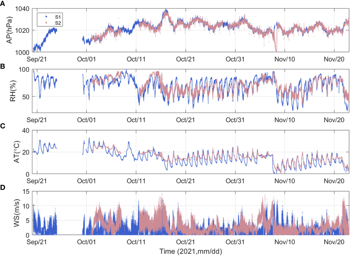
Figure 3 Observed atmospheric parameters at Rizhao and Yancheng from September 20 to November 22, 2021: (A) air pressure, (B) relative humidity, (C) air temperature, and (D) wind speed.

3.2 Statistical properties of measured PL

The cumulative distribution function (CDF) is used in the statistical analysis of the measured PL. The CDF of the random variable  X has the following definition:

where P(X≤t) represents the probability of a random variable X which takes the value that is less than or equal to that of the t . The CDF is used to determine the likelihood that a random observation taken from the population will be less than or equal to a particular value.

Table 2 presents some basic statistical characteristics of the measured PL, and Figure 4 shows the empirical CDF of the measured PL during different months. With the maximum measurable power loss of 200 dB, our measurement system connected with a probability of 52.6% during the measurement period. The PL higher than 200dB was noise, and we only show the CDF of PL below 200dB. The PL distribution of three months in autumn is basically the same as shown in Figure 4. The probabilities of PL of less than 200 dB were 85.9% in September. However, since the measurement in September started on September 20, 2021, and only lasted for about 10 days, the statistical results of this month may not be representative. The probabilities of PL of less than 200 dB were 48.2% in October, and 53.2% in November, respectively. The mean values of PL were 189 dB in September, 195 dB in October, and 192 dB in November, respectively. The probabilities of PL of less than 200, 190, 180, and 170 dB during the measurement period were 52.6%, 31.3%, 18.5%, and 7.3%, respectively.

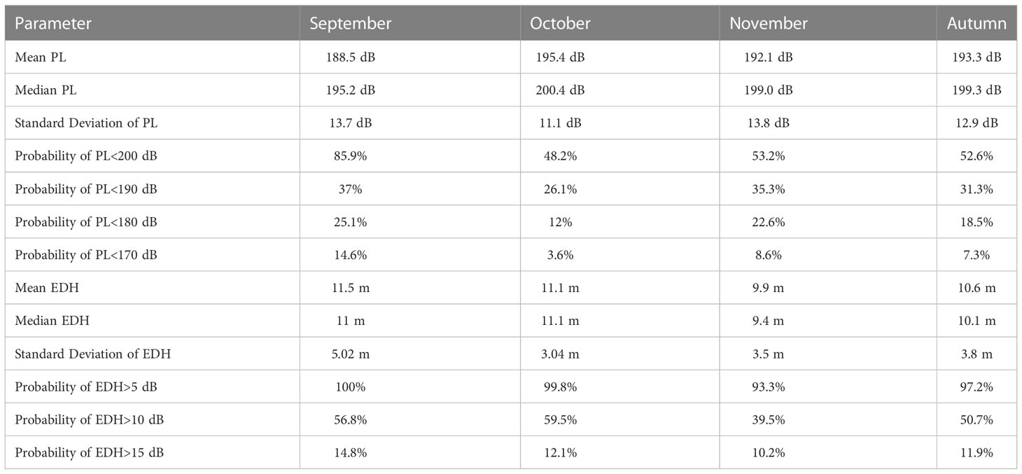
Table 2 Statistical characteristics of measured PL and simulated EDH at P3 during the measurement.

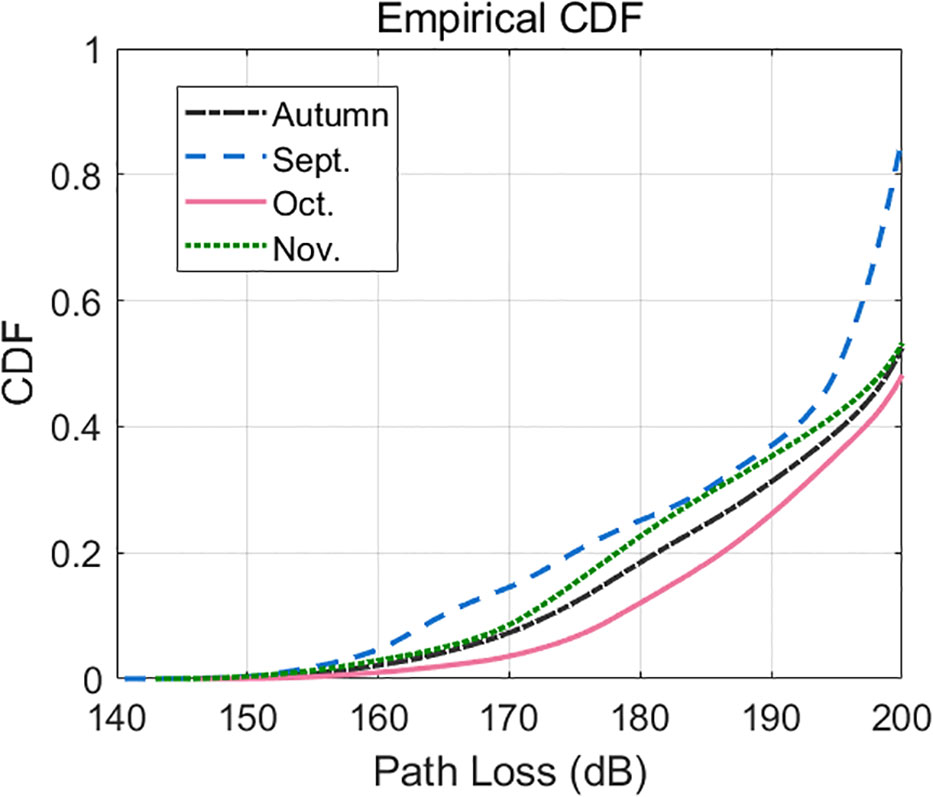
Figure 4 Empirical CDF of measured PL during different months.

For a communication system, the communication system capability A is defined as follows (Yang et al., 2021):

where P_t is the Tx power, G_t is the Tx antenna gain, G_r is the Rx antenna gain, L is receiver sensitivity, SL is the system loss, and M is the system margin.

Thus, for a communication system with system capacity of 190 dB, the available signal probability over 133 km in the Yellow Sea was approximately 31.3% during the measurement period. For a real-time communication system, this available signal probability obviously cannot meet the requirements; however, over-the-horizon communication capability can be improved by shortening the propagation distance or by increasing the communication system capability. For quasi-real-time communication systems, such as observation buoys, over-the-horizon communication could be achieved during the better communication environments when the EDH is high causing small PL and large throughput can be achieved.

3.3 Evaporation duct climatology during the measurement period

The evaporation duct distributions during the measurement period were obtained using the ECMWF ERA5 reanalysis data. It can be seen from Figure 5A that EDH varied dramatically during the measurement period. However, there was little difference in EDH at different positions along the link, which reflects characteristics of horizontal inhomogeneity. The reason that PL distribution is basically the same in autumn is that the climatic conditions are basically the same, which leads to similar distribution of EDHs. Table 2 presents some statistical characteristics of the simulated EDH at P3 during the measurement. The mean EDHs were 11.5m in September, 11.1 m in October, and 9.9 m in November. Variations in EDH over the ocean come primarily from variations in four environmental parameters: SST, AT, RH, and near-surface WS. The regular monthly variation of environmental parameters leads to the monthly variation of the EDH to be general, except in some extreme weather conditions. The mean value of EDH at P3 during the measurement period was 10.6 m, which was relatively low. This led to a small probability of communication via the over-the-horizon link in autumn. Figure 5B shows the empirical CDF of EDH at P3 during the measurement period. The probabilities of EDH greater than 5, 10, and 15 m during the measurement period were 97.2%, 50.7%, and 11.9%, respectively.

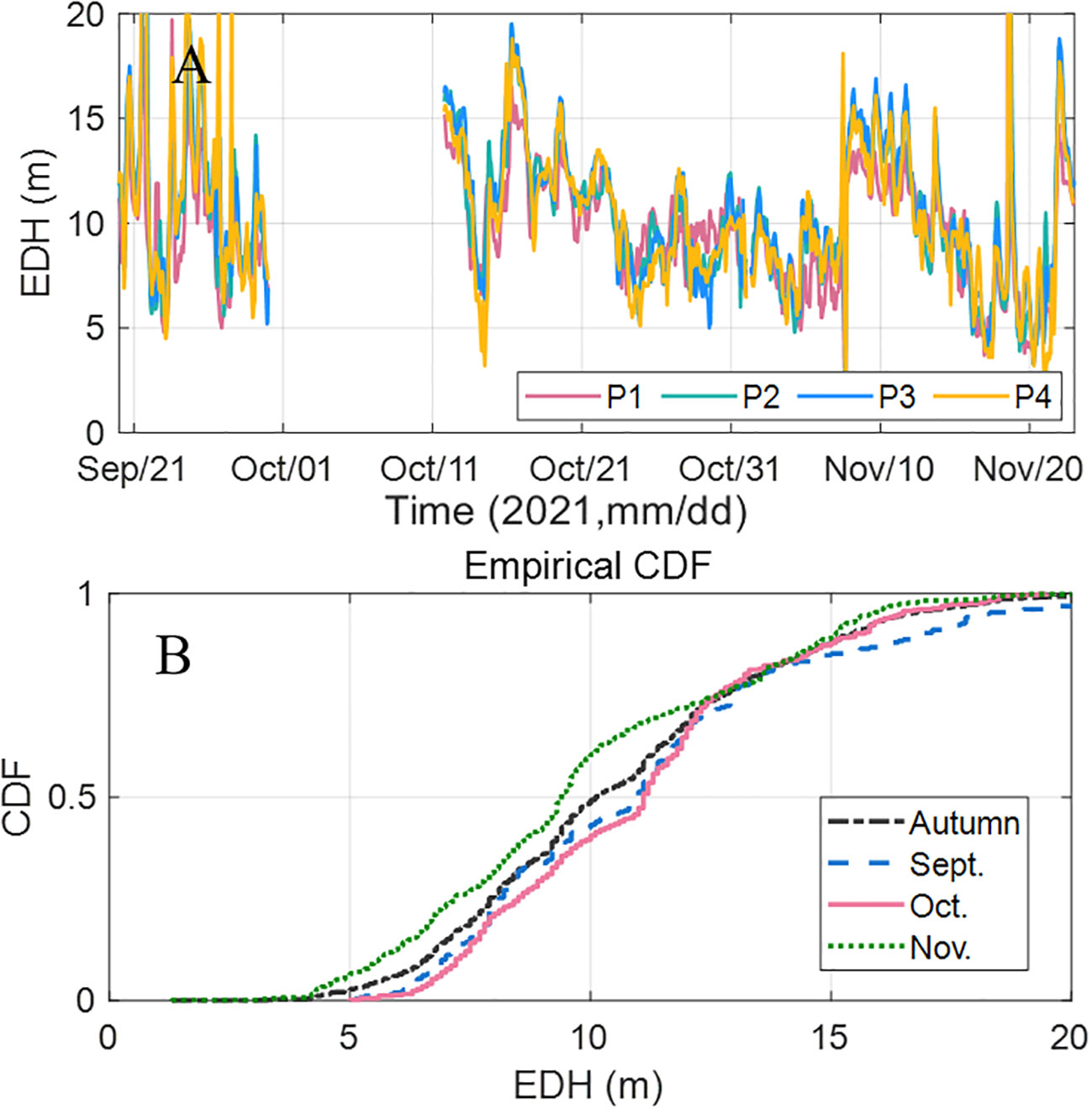
Figure 5 (A) EDH distribution and (B) empirical CDF of EDH at P3 during the measurement period.

3.4 Duct effect and model evaluation

The effect of evaporation ducts on the over-the-horizon propagation link are analyzed in this section. The M-profiles calculated by NAVSLaM using the ERA5 data were input into the APM to simulate PL during the measurement period. Data for sites P4, P3, P2, and P1, shown in Figure 1A, were used as inputs into the models. For clarity, we present the results of November as an example to study the influence of evaporation ducts on the over-the-horizon link. Figure 6A shows the range-dependent M-profiles along the propagation link at 08:00 on November 10, 2021. The black curves are the M-profiles at different propagation distances. The red circles are the positions of minimum values of the M, and the corresponding height is the EDHs. Figure 6B shows the PL computed using APM and ray traces computed using the ray-optics approach (Zhou et al., 2018) based on the range-dependent modified refractivity profile. The simulation parameters are shown in Table 1. For clarity, individual rays are traced and shown in black. It is shown that the results obtained using these two approaches is consistent with each other. The rays are strongly refracted towards the earth, followed by reflection off the earth surface only to be refracted back down. In other words, the rays are trapped, resulting in low PL beyond the horizon relative to the normal atmosphere. Figure 6C is extracted from the PL computed using APM in Figure 6B by fixing the Rx height to 3m, which shows the PL vs range from 0-133km. The PL is about 129 dB at 20 km. The PL at 120 km is about 142 dB, which is only 13-dB higher than that at 20 km. The PL exponent (Rouphael, 2009) is about 1.709.

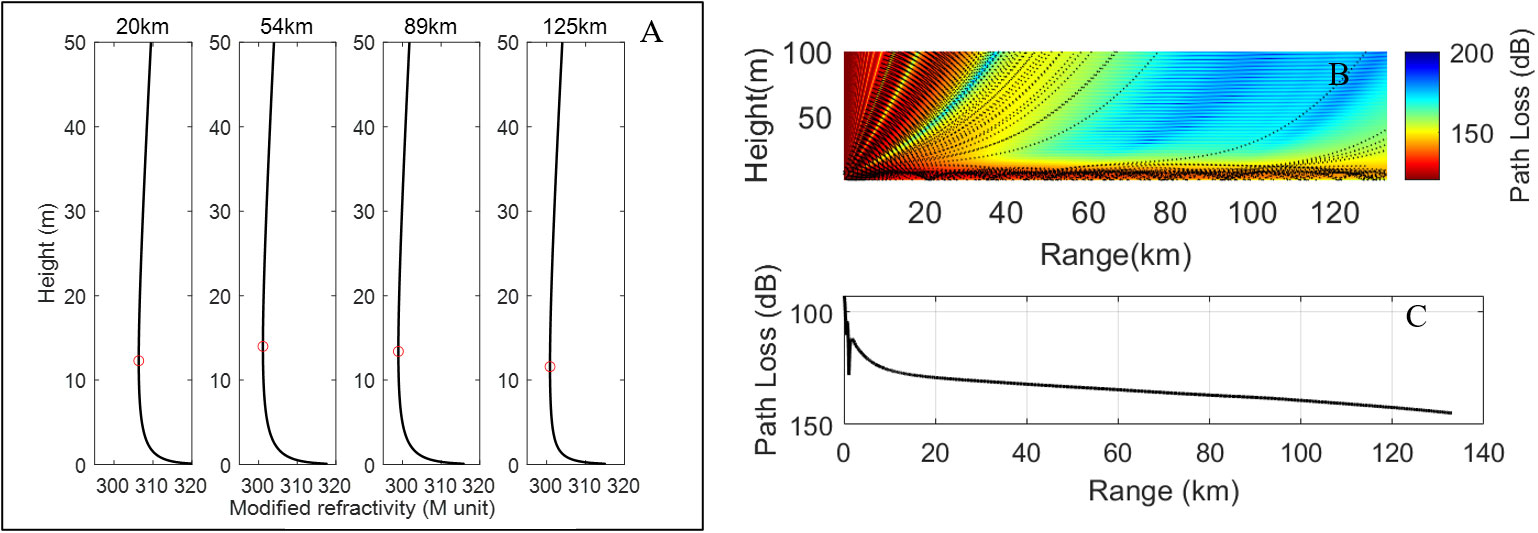
Figure 6 (A) Modified refractivity profiles at different propagation distances at 08:00 on November 10, 2021. The black curves are the M-profiles. The red circles are the positions of minimum values of the M, and the corresponding height is the EDHs. (B) the PLs and ray traces based on the range-dependent modified refractivity profile. (C) the PL vs range at Rx height 3m, Tx height 6m, and frequency 9.4GHz.

The measured PL and the simulation results obtained from different PL models are presented in Figure 7 for comparison. For the 133-km link, the PL of the free space was 154 dB obtained by equation (8), while that of the 2-Ray model was 181 dB obtained by equation (9). The free space loss model and 2-Ray model do not consider the effect of evaporation duct. The APM can reflect the trapping effect of the evaporation duct on the EM waves, and it could be used to predict the trend of the measured PL. Correlation analysis showed the correlation coefficient between the simulated PL and the measured PL is 0.57. However, sometimes the prediction error was still large. For example, the prediction errors were large during 8-12 November. Although the model estimated that over-the-horizon signal can be detected at that time, it underestimated the PL. The possible reasons for the large prediction error are: 1) input environmental data deviation. Since the ECMWF data are reanalyzed data, there may be some errors in it, resulting in large prediction errors at some points; 2) NAVSLaM and the APM model prediction errors in some environments, such as extremely high and extremely low WS, atmospheric stable conditions (air-sea temperature difference (ASTD)>0);3) lack of modeling propagation environments such as rainfall, waves, tides, and local random weather process.

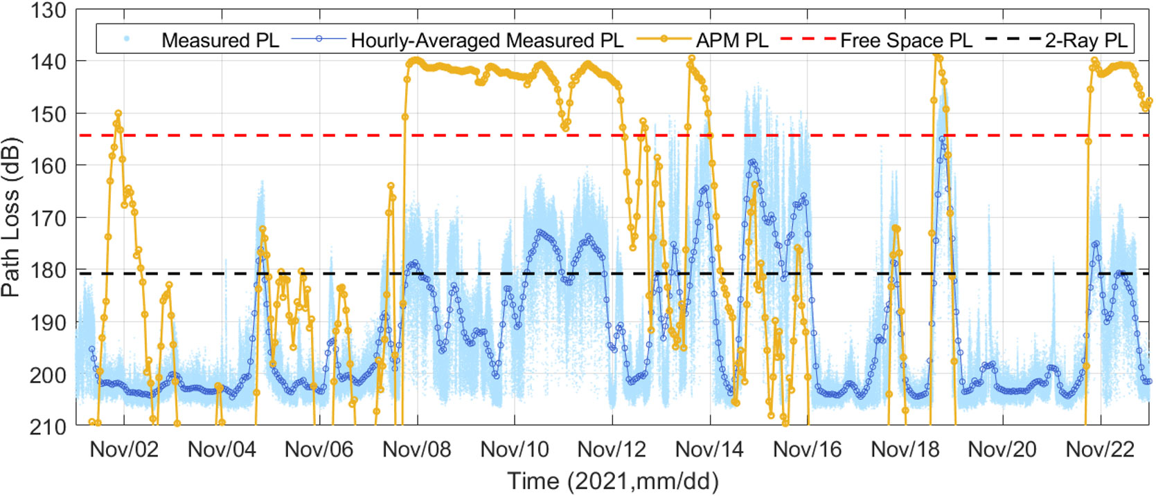
Figure 7 Comparison between measured PL and PL simulated by different models.

Figure 8 shows the correlation between the absolute error (AE) of the predicted PL and air–sea parameters when the measured PL was<200 dB during the entire measurement period. The absolute error AE of PL is defined as: AE_PL=|PL_measured−PL_predicted| . As shown in Figure 8D, the AE of the predicted PL was larger when the predicted EDH was either too low or too high. The AE of the predicted PL was smaller when the EDH was approximately 10 m. This means that the simulation model overestimated PL when EDH was low but underestimated PL when EDH was high, which led to many extreme values in the results. The correlations between the AE of the predicted PL and both the ASTD and the WS also indicated that EDH would be large when the absolute value of the ASTD was large and the WS was high, and also EDH would be low when the absolute value of the ASTD was small and the WS was low, both leading to greater prediction error. In summary, for an over-the-horizon link, the actual structure of an evaporation duct is horizontal inhomogeneous, caused by the difference between large-scale air–sea conditions and the locally random weather process. These complex environments cannot be well modeled. Therefore, the physics prediction models show some limitations in practice, as well as problems such as poor stability and large prediction errors in general, especially for an over-the-horizon propagation link.

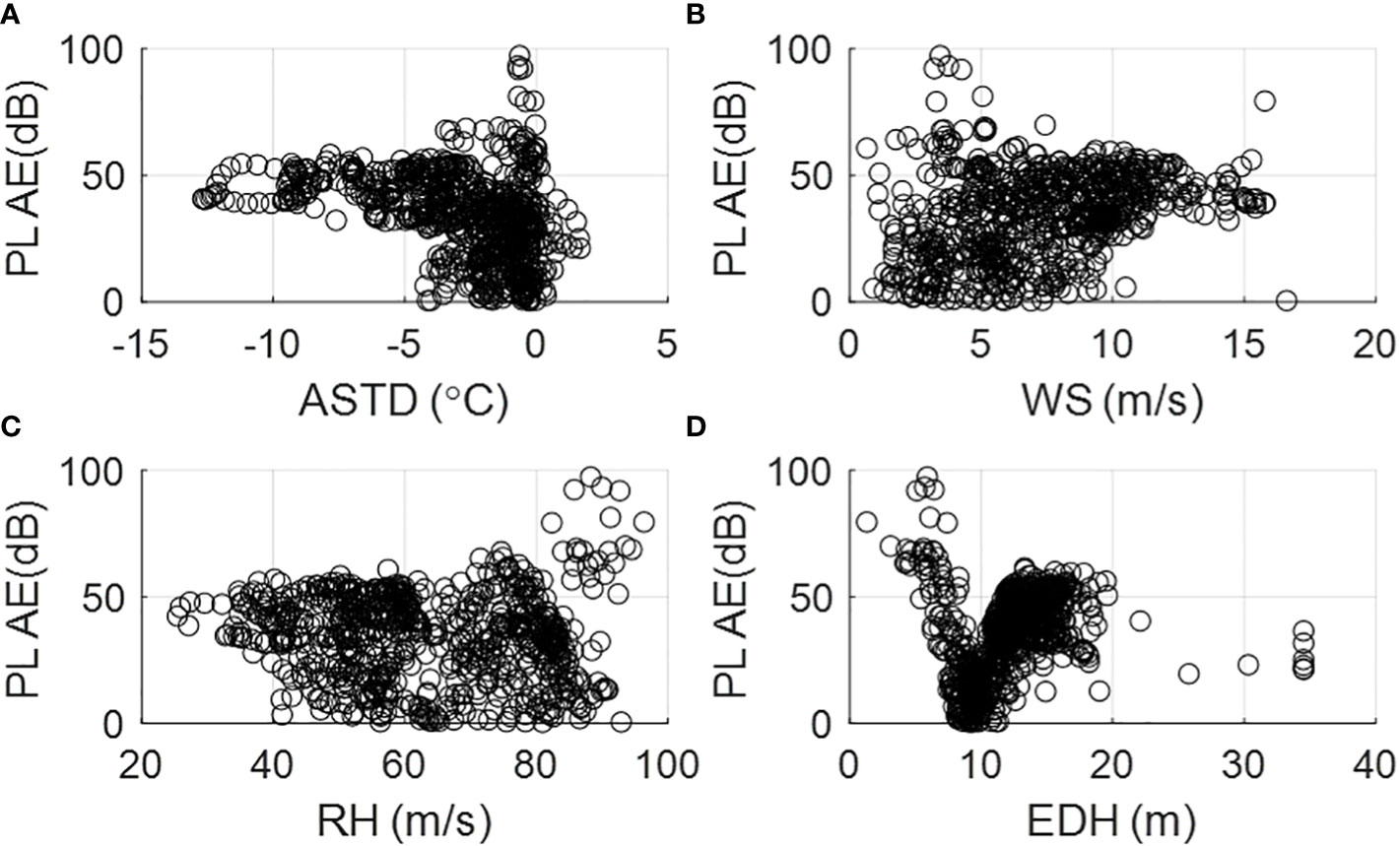
Figure 8 Correlation between absolute error of predicted PL and air–sea parameters: (A) air-sea temperature difference, (B) wind speed, (C) relative humidity, and (D) EDH.

3.5 Example analysis of abnormal PL decrease

In this section, an example analysis explores some reasons for the decrease of PL of the over-the-horizon EM propagation link in the Yellow Sea in autumn. As shown in Figure 7, over-the-horizon propagation occurred during November 8–12 with low PL. Figure 9 shows the evolutions of air–sea parameters during November 6–12. As shown in Figure 9F, EDH increased from 7 to 15 m during November 6–8. The main reasons for the increase in EDH were reduction in RH, increase in WS, and increase in ASTD, which promoted evaporation of seawater. The reason for this series of changes in the meteorological parameters was that the wind changed from a sea breeze to a land breeze, as shown in Figure 9C. Figure 10 shows the changes of WS and wind direction (WD) during this period. The land breeze introduced dry and cold air to the link, which promoted evaporation of seawater and reduced the PL. Analysis of the over-the-horizon propagation examples during the measurement period revealed that factors such as increase in WS and reduction in RH were the main reasons for the increase in EDH and reduction in PL.

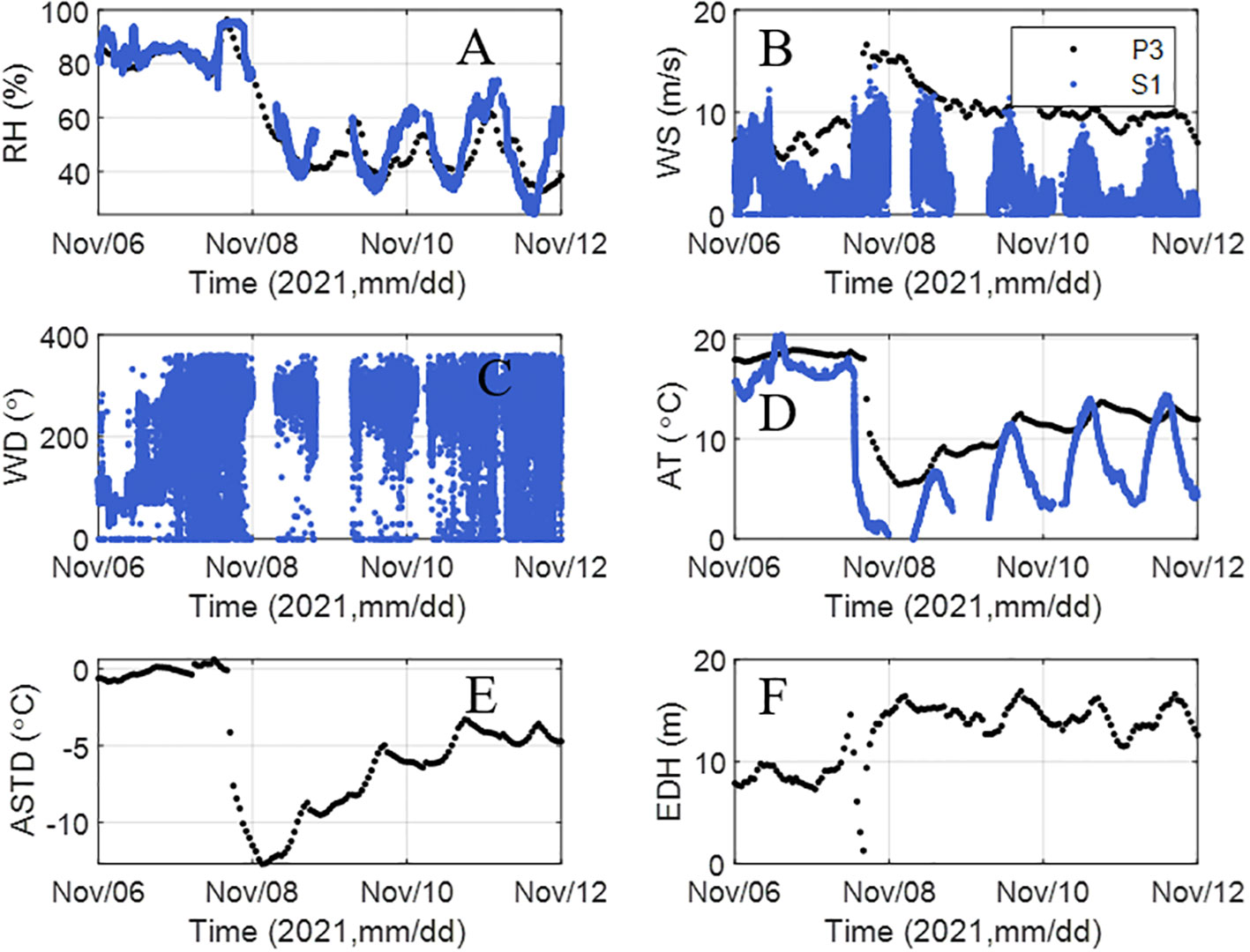
Figure 9 Evolution of air–sea parameters during November 6–12, 2021: (A) relative humidity, (B) wind speed, (C) wind direction, (D) air temperature, (E) air-sea temperature difference, and (F) EDH.

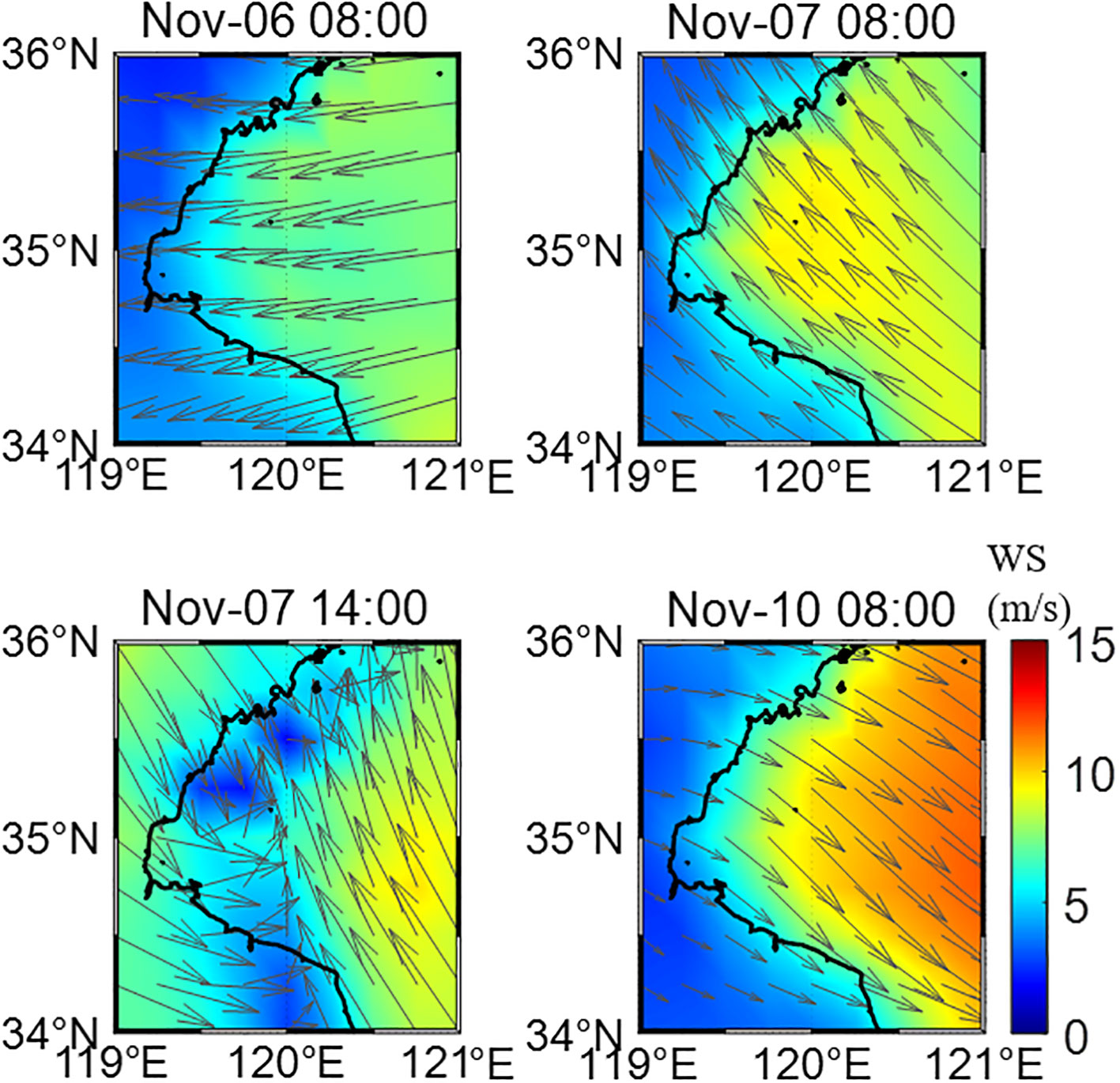
Figure 10 Evolutions of wind during November 6–10, 2021.

4 Discussion

In this section, the spatiotemporal characteristics of EDH during different months in the Yellow Sea are presented. Figure 11 shows the monthly average EDH in 2021 over the Yellow Sea. The monthly averaged EDH distributions show strong inhomogeneity. For example, EDH was low in December-January (<10 m) and high in April–June; it was highest in May (average value: >15 m). During March–June, EDH in the northern part of the Yellow Sea was much higher than that in the southern part. Variations in EDH over the ocean come primarily from variations in four environmental parameters: SST, AT, RH, and near-surface WS (McKeon, 2013). Except for some extreme weather conditions, the monthly variation of EDH is general due to the regular monthly distributions of environmental parameters. The main reason for the high EDH in May is because the ASTD is larger than 0°C and lead to stable atmospheric conditions in May (Yang et al., 2016).

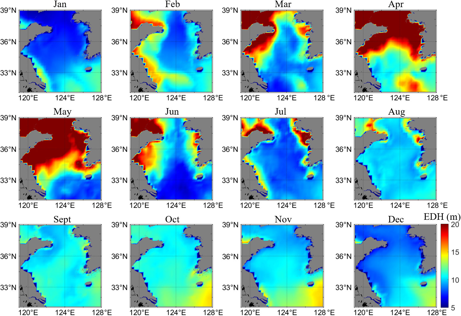
Figure 11 Monthly averaged EDH in 2021 over the Yellow Sea.

Figure 12 shows the monthly probability density function (PDF) of EDH at P3 in 2021. The distribution of EDH in April–June was reasonably uniform with higher values of EDH. Figure 13A shows the mean EDH in different months at P3. The highest mean EDH was in May with an average value of 15.7 m. During our measurement period, the mean EDH was 10.6, 11.1, and 9.6 m in September, October, and November, respectively. The low values of mean EDH in December (8 m) and January (8.6 m) indicate that the conditions were unsuitable for over-the-horizon communication. Figure 13B shows the monthly CDF of EDH in 2021 over the Yellow Sea. In May, the probabilities of EDH being greater than 10, 15, and 20 m were 62%, 47%, and 30% respectively. The CDF of EDH can provide the basis for evaluation of the performance of an over-the-horizon system. Overall, in the Yellow Sea, spring is the optimum time for over-the-horizon high-speed communication using evaporation ducts.

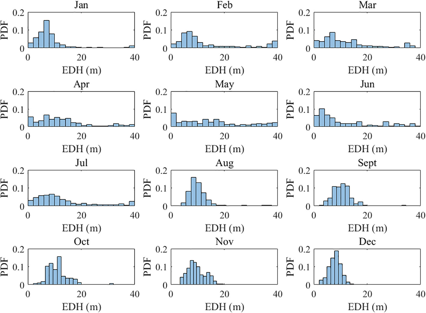
Figure 12 Monthly PDF of EDH in 2021 over the Yellow Sea at P3.

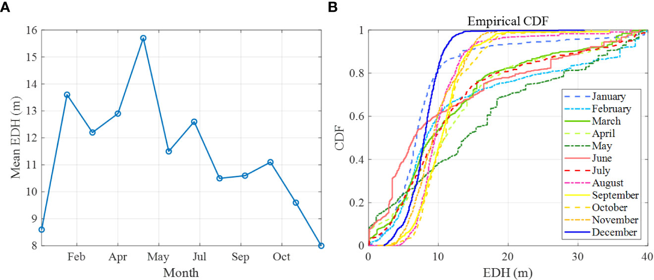
Figure 13 EDH statistical characteristics. (A) mean EDH of different months at P3, (B) monthly CDF of EDH in 2021 over the Yellow Sea.

5 Conclusions

Long-term measurements of over-the-horizon microwave propagation in evaporation ducts over the Yellow Sea in 2021 were presented in this paper. The results were analyzed on the basis of statistical analysis and model simulations. The derived conclusions are as follows.

1) For a 133-km-long link (7.7 times the line-of-sight length), the probabilities of PL of less than 200, 190, and 180 dB during the measurement period were 52.6%, 31.3%, and 18.5%, respectively.

2) Obtained using the ECMWF ERA5 reanalysis data and the NAVSLaM, the probabilities of EDH being greater than 5, 10, and 15 m during the measurement period were 97.2%, 50.7%, and 11.9%, respectively. Evaporation duct environments in autumn are not ideal for long-range EM propagation. The model prediction method is unreliable and produces some extreme values when EDH is either too low or too high.

3) A land breeze in autumn will introduce dry and cold air to the link, which can promote evaporation of seawater and reduce the PL by approximately 40 dB. Factors such as increase in WS and reduction in RH were the main reasons for the increase in EDH and reduction in PL during the measurement period.

4) In the Yellow Sea, evaporation ducts are most suitable for over-the-horizon communication in spring, especially May.

Data availability statement

The original contributions presented in the study are included in the article/Supplementary Material. Further inquiries can be directed to the corresponding author.

Author contributions

Conceptualization, KY; methodology, SW; software, SW and YS; validation, SW; formal analysis, SW; investigation, YS, HZ, and FY; field measurements, SW, FY, DH, GD, and YHS; resources, DH; data curation, SW and GD; writing—original draft preparation, SW; writing—review and editing, KY and YS; supervision, KY; project administration, KY and YS; funding acquisition, SW, KY, YS, and HZ. All authors contributed to the article and approved the submitted version.

Funding

This work was supported in part by Innovation Foundation for Doctor Dissertation of Northwestern Polytechnical University under Grant CX2022008; and in part by the National Natural Science Foundation of China under Grant 42076198, Grant 41906160 and Grant 42176190; and in part by the Innovation Capability Support Program of Shaanxi under Grant 2022KJXX-76; and in part by the Fundamental Research Funds for the Central Universities under Grant 3102021HHZY030010.

Conflict of interest

The authors declare that the research was conducted in the absence of any commercial or financial relationships that could be construed as a potential conflict of interest.

Publisher’s note

All claims expressed in this article are solely those of the authors and do not necessarily represent those of their affiliated organizations, or those of the publisher, the editors and the reviewers. Any product that may be evaluated in this article, or claim that may be made by its manufacturer, is not guaranteed or endorsed by the publisher.

Abbreviations

AE, absolute error; AP, air pressure; APM, advanced propagation model; ASTD, air–sea temperature difference; AT, air temperature; CDF, cumulative distribution function; ECMWF, European Centre for Medium-Range Weather Forecasts; EDH, evaporation duct height; EM, electromagnetic; NAVSLaM, naval atmospheric vertical surface layer model; PDF, probability density function; PE, parabolic equation; PL, path loss; RH, relative humidity; RSL, received signal level; SST, sea surface temperature; WD, wind direction; WS, wind speed.

References

Anderson K., Brooks B., Caffrey P., Clarke A., Cohen L., Crahan K., et al. (2004). The RED experiment: An assessment of boundary layer effects in a trade winds regime on microwave and infrared propagation over the Sea. Bull. Amer. Meteor. Soc 85, 1355–1366. doi: 10.1175/BAMS-85-9-1355
Babin S. M. (1996). A new model of the oceanic evaporation duct and its comparison with current models. Ph.D. Thesis, (USA: University of Maryland, College Park, MD).
Babin S. M., Dockery G. D. (2002). LKB-based evaporation duct model comparison with buoy data. J. Appl. Meteor. 41, 434–446. doi: 10.1175/1520-0450(2002)041<0434:LBEDMC>2.0.CO;2
Barrios A. E. (1994). A terrain parabolic equation model for propagation in the troposphere. IEEE Trans. Antennas Propagat. 42, 90–98. doi: 10.1109/8.272306
Barrios A., Patterson W., Sprague R. (2002). Advanced propagation model (APM) version 2.1.04 computer software configuration item (CSCI) documents. (San Diego: Space and Naval Warfare Systems Command).
Couillard D., Dahman G., GrandMaison M.-E., Poitau G., Gagnon F. (2018). Robust broadband maritime communications: Theoretical and experimental validation. Radio Sci. 53, 749–760. doi: 10.1029/2018RS006561
Fairall C. W., Bradley E. F., Hare J. E., Grachev A. A., Edson J. B. (2003). Bulk parameterization of air–Sea fluxes: Updates and verification for the COARE algorithm. J. Climate 16, 571–591. doi: 10.1175/1520-0442(2003)016<0571:BPOASF>2.0.CO;2
Frederickson P. A., Davidson K. L., Goroch A. K. (2000). Operational bulk evaporation duct model for MORIAH version 1.2 (Monterey, CA, USA: Nav. PostgraduateSchool).
Goldhirsh J., Dockery D. (1998). Propagation factor errors due to the assumption of lateral homogeneity. Radio Sci. 33, 239–249. doi: 10.1029/97RS03321
Haus B. K., Ortiz-Suslow D. G., Doyle J. D., Flagg D. D., Graber H. C., MacMahan J., et al. (2022). CLASI: Coordinating innovative observations and modeling to improve coastal environmental prediction systems. Bull. Amer. Meteor. Soc 103, E889–E898. doi: 10.1175/BAMS-D-20-0304.1
Hersbach H., Bell B., Berrisford P., Hirahara S., Horányi A., Muñoz-Sabater J., et al. (2020). The ERA5 global reanalysis. Q.J.R. Meteorol. Soc 146, 1999–2049. doi: 10.1002/qj.3803
Hitney H. V., Hitney L. R. (1990). Frequency diversity effects of evaporation duct propagation. IEEE Trans. Antennas Propagat. 38, 1694–1700. doi: 10.1109/8.59784
Huang L., Zhao X., Liu Y., Yang P., Ding J., Zhou Z. (2022). The diurnal variation of the evaporation duct height and its relationship with environmental variables in the south China Sea. IEEE Trans. Antennas Propagat. 70, 10865–10875. doi: 10.1109/TAP.2022.3191160
Kulessa A. S., Barrios A., Claverie J., Garrett S., Haack T., Hacker J. M., et al. (2017). The tropical air–Sea propagation study (TAPS). Bull. Amer. Meteor. Soc 98, 517–537. doi: 10.1175/BAMS-D-14-00284.1
Lee Y. H., Dong F., Meng Y. S. (2014). Near Sea-surface mobile radiowave propagation at 5 GHz: Measurements and modeling. Radioengineering 23, 824–830.
Ma J., Wang J., Yang C. (2022). Long-range microwave links guided by evaporation ducts. IEEE Commun. Mag. 60, 68–72. doi: 10.1109/MCOM.002.00508
McKeon B. D. (2013) Climate analysis of evaporation ducts in the south China Sea. Available at: http://hdl.handle.net/10945/38983.
Musson-Genon L., Gauthier S., Bruth E. (1992). A simple method to determine evaporation duct height in the sea surface boundary layer. Radio Sci. 27, 635–644. doi: 10.1029/92RS00926
Ozgun O., Sahin V., Erguden M. E., Apaydin G., Yilmaz A. E., Kuzuoglu M., et al. (2020). PETOOL v2.0: Parabolic equation toolbox with evaporation duct models and real environment data. Comput. Phys. Commun. 256, 107454. doi: 10.1016/j.cpc.2020.107454
Paulus R. A. (1985). Practical application of an evaporation duct model. Radio Sci. 20, 887–896. doi: 10.1029/RS020i004p00887
Pozderac J., Johnson J., Yardim C., Merrill C., de Paolo T., Terrill E., et al. (2018). X-Band beacon-receiver array evaporation duct height estimation. IEEE Trans. Antennas Propagat. 66, 2545–2556. doi: 10.1109/TAP.2018.2814060
Robinson L., Newe T., Burke J., Toal D. (2022). A simulated and experimental analysis of evaporation duct effects on microwave communications in the Irish Sea. IEEE Trans. Antennas Propagat. 70, 4728–4737. doi: 10.1109/TAP.2022.3145460
Rouphael T. J. (2009). “Chapter 4 - high-level requirements and link budget analysis,” in RF and digital signal processing for software-defined radio. Ed. Rouphael T. J. (Burlington: Newnes), 87–122. doi: 10.1016/B978-0-7506-8210-7.00004-7
Shi Y., Kun-De Y., Yang Y.-X., Ma Y.-L. (2015a). Influence of obstacle on electromagnetic wave propagation in evaporation duct with experiment verification. Chin. Phys. B 24, 54101. doi: 10.1088/1674-1056/24/5/054101
Shi Y., Yang K., Yang Y., Ma Y. (2015b). A new evaporation duct climatology over the south China Sea. J. Meteorol Res. 29, 764–778. doi: 10.1007/s13351-015-4127-6
Shi Y., Yang K.-D., Yang Y.-X., Ma Y.-L. (2015c). Experimental verification of effect of horizontal inhomogeneity of evaporation duct on electromagnetic wave propagation. Chin. Phys. B 24, 44102. doi: 10.1088/1674-1056/24/4/044102
Shi Y., Zhang Q., Wang S., Yang K., Yang Y., Yan X., et al. (2019). A comprehensive study on maximum wavelength of electromagnetic propagation in different evaporation ducts. IEEE Access 7, 82308–82319. doi: 10.1109/ACCESS.2019.2923039
Sirkova I. (2015). Duct occurrence and characteristics for Bulgarian black sea shore derived from ECMWF data. J. Atmospheric Solar-Terrestrial Phys. 135, 107–117. doi: 10.1016/j.jastp.2015.10.017
Smith E., Weintraub S. (1953). The constants in the equation for atmospheric refractive index at radio frequencies. Proc. IRE 41, 1035–1037. doi: 10.1109/JRPROC.1953.274297
Ulate M., Wang Q., Haack T., Holt T., Alappattu D. P. (2019). Mean offshore refractive conditions during the CASPER East field campaign. J. Appl. Meteorology Climatology 58, 853–874. doi: 10.1175/JAMC-D-18-0029.1
Wang Q., Alappppattu D. P., Billingsley S., Blomquist B., Burkholder R. J., Christman A. J., et al. (2018). CASPER: Coupled air-Sea processes and electromagnetic ducting research. Bull. Amer. Meteorol. Soc. 99, 1449–1471. doi: 10.1175/bams-d-16-0046.1
Wang Q., Burkholder R. J., Yardim C., Xu L., Pozderac J., Christman A., et al. (2019). Range and height measurement of X-band EM propagation in the marine atmospheric boundary layer. IEEE Trans. Antennas Propagat. 67, 2063–2073. doi: 10.1109/tap.2019.2894269
Wang S., Han J., Shi Y., Yang K., Huang C., Yang F. (2020). The influence of antenna height on microwave propagation in evaporation duct. In Global Oceans 2020: Singapore – U.S. Gulf Coast. 1–5. doi: 10.1109/IEEECONF38699.2020.9389404
Wang S., Yang K., Shi Y., Yang F. (2022a). Observations of Anomalous Over-the-Horizon Propagation in the Evaporation Duct Induced by Typhoon Kompasu, (202118). IEEE Antennas Wireless Propagation Lett. 21, 963–967. doi: 10.1109/LAWP.2022.3153389
Wang S., Yang K., Shi Y., Yang F., Zhang H. (2022b). Impact of evaporation duct on electromagnetic wave propagation during a typhoon. J. Ocean Univ. China 21, 1069–1083. doi: 10.1007/s11802-022-4967-5
Woods G. S., Ruxton A., Huddlestone-Holmes C., Gigan G. (2009). High-capacity, long-range, over ocean microwave link using the evaporation duct. IEEE J. Oceanic Eng. 34, 323–330. doi: 10.1109/JOE.2009.2020851
Xu L., Yardim C., Mukherjee S., Burkholder R. J., Wang Q., Fernando H. J. S. (2022). Frequency diversity in electromagnetic remote sensing of lower atmospheric refractivity. IEEE Trans. Antennas Propagat. 70, 547–558. doi: 10.1109/TAP.2021.3090828
Yang C., Shi Y., Wang J., Feng F. (2022a). Regional spatiotemporal statistical database of evaporation ducts over the south China Sea for future long-range radio application. IEEE J. Sel. Top. Appl. Earth Observations Remote Sens. 15, 6432–6444. doi: 10.1109/JSTARS.2022.3197406
Yang C., Wang J., Feng F. (2021). The statistical distributions of evaporation duct and the communication characteristics over the south China Sea. Earth Space Sci. Open Arch. 1–30. doi: 10.1002/essoar.10507619.1
Yang C., Wang J., Ma J. (2022b). Exploration of X-Band communication for maritime applications in the south China Sea. Antennas Wirel. Propag. Lett. 21, 481–485. doi: 10.1109/LAWP.2021.3136044
Yang F., Yang K., Shi Y., Wang S., Zhang H., Zhao Y. (2022c). The effects of rainfall on over-the-Horizon propagation in the evaporation duct over the south China Sea. Remote Sens. 14, 4787. doi: 10.3390/rs14194787
Yang K., Zhang Q., Shi Y., He Z., Lei B., Han Y. (2016). On analyzing space-time distribution of evaporation duct height over the global ocean. Acta Oceanol. Sin. 35, 20–29. doi: 10.1007/s13131-016-0903-0
Zaidi K. S., Hina S., Jawad M., Khan A. N., Khan M. U. S., Pervaiz H. B., et al. (2021). Beyond the horizon, backhaul connectivity for offshore IoT devices. Energies 14, 6918. doi: 10.3390/en14216918
Zhang Q., Wang S., Shi Y., Yang K. (2022). Measurements and analysis of maritime wireless channel at 8GHz in the south China Sea region. IEEE Trans. Antennas Propagat., 1–1. doi: 10.1109/TAP.2022.3209664
Zhang Q., Yang K., Shi Y. (2016). Spatial and temporal variability of the evaporation duct in the gulf of Aden. Tellus A: Dynamic Meteorology Oceanography 68, 29792. doi: 10.3402/tellusa.v68.29792
Keywords: channel measurement, evaporation duct, over-the-horizon, maritime communication, microwave propagation
Citation: Wang S, Yang K, Shi Y, Zhang H, Yang F, Hu D, Dong G and Shu Y (2023) Long-term over-the-horizon microwave channel measurements and statistical analysis in evaporation ducts over the Yellow Sea. Front. Mar. Sci. 10:1077470. doi: 10.3389/fmars.2023.1077470
Received: 23 October 2022; Accepted: 10 January 2023;
Published: 26 January 2023.
Edited by:
Kun Yang, Zhejiang Ocean University, ChinaCopyright © 2023 Wang, Yang, Shi, Zhang, Yang, Hu, Dong and Shu. This is an open-access article distributed under the terms of the Creative Commons Attribution License (CC BY). The use, distribution or reproduction in other forums is permitted, provided the original author(s) and the copyright owner(s) are credited and that the original publication in this journal is cited, in accordance with accepted academic practice. No use, distribution or reproduction is permitted which does not comply with these terms.
*Correspondence: Yang Shi, shiyang@nwpu.edu.cn