Using Predicted Patterns of 3D Prey Distribution to Map King Penguin Foraging Habitat
 Roland Proud1*
  Camille Le Guen1
  Richard B. Sherley2,3
  Akiko Kato4
  Yan Ropert-Coudert4
  Norman Ratcliffe5
  Simon Jarman6
  Adam Wyness7
  John P. Y. Arnould8
  Ryan A. Saunders5
  Paul G. Fernandes9 Lars Boehme10
  Andrew S. Brierley1
- 1Pelagic Ecology Research Group, Scottish Oceans Institute, School of Biology, Gatty Marine Laboratory, University of St Andrews, St Andrews, United Kingdom
- 2Centre for Ecology and Conservation, University of Exeter, Penryn, United Kingdom
- 3FitzPatrick Institute of African Ornithology, DST-NRF Centre of Excellence, University of Cape Town, Rondebosch, South Africa
- 4Centre d’Etudes Biologiques de Chizé, UMR 7372 CNRS-La Rochelle Université, Villiers en Bois, France
- 5British Antarctic Survey, Cambridge, United Kingdom
- 6School of Biological Sciences, University of Western Australia, Perth, WA, Australia
- 7Coastal Research Group, Department of Zoology and Entomology, Rhodes University, Grahamstown, South Africa
- 8School of Life and Environmental Sciences, Deakin University, Burwood, VIC, Australia
- 9School of Biological Sciences, University of Aberdeen, Aberdeen, United Kingdom
- 10Scottish Oceans Institute, School of Biology, Gatty Marine Laboratory, University of St Andrews, St Andrews, United Kingdom
King penguins (Aptenodytes patagonicus) are an iconic Southern Ocean species, but the prey distributions that underpin their at-sea foraging tracks and diving behaviour remain unclear. We conducted simultaneous acoustic surveys off South Georgia and tracking of king penguins breeding ashore there in Austral summer 2017 to gain insight into habitat use and foraging behaviour. Acoustic surveys revealed ubiquitous deep scattering layers (DSLs; acoustically detected layers of fish and other micronekton that inhabit the mesopelagic zone) at c. 500 m and shallower ephemeral fish schools. Based on DNA extracted from penguin faecal samples, these schools were likely comprised of lanternfish (an important component of king penguin diets), icefish (Channichthyidae spp.) and painted noties (Lepidonotothen larseni). Penguins did not dive as deep as DSLs, but their prey-encounter depth-distributions, as revealed by biologging, overlapped at fine scale (10s of m) with depths of acoustically detected fish schools. We used neural networks to predict local scale (10 km) fish echo intensity and depth distribution at penguin dive locations based on environmental correlates, and developed models of habitat use. Habitat modelling revealed that king penguins preferentially foraged at locations predicted to have shallow and dense (high acoustic energy) fish schools associated with shallow and dense DSLs. These associations could be used to predict the distribution of king penguins from other colonies at South Georgia for which no tracking data are available, and to identify areas of potential ecological significance within the South Georgia and the South Sandwich Islands marine protected area.
Introduction
The Southern Ocean is one of the most pristine ecosystems on the planet. At present, 7.2% of the ocean surface is protected, and this may expand to 11.2% if proposed marine protected areas (MPAs) are sanctioned (Hindell et al., 2020). As part of the Global Ocean Alliance push for ‘30 by 30’, there is an aspiration to afford protection to more. Understanding the distribution of predators at sea is part of the process of developing spatial management plans. Hindell et al. (2020) proposed areas of ecological significance (AESs) based on predator tracks, but these AESs do not consider prey distributions directly. Determining how marine predators find their prey and hence better understanding their foraging ecology and role in ocean food webs is important for marine conservation.
Foraging habitat choices by central-place foragers during the breeding season are determined by their colony locations and dive capabilities, relative to the three-dimensional spatial distributions of prey (that may themselves show diel or seasonal variability due to migration) and competition with conspecifics and other predator species (Fauchald, 2009; Boyd et al., 2015). In turn, the self-organising behaviour of prey into, e.g., schools, swarms, patches and layers for protection from predation (Brierley and Cox, 2015; Rieucau et al., 2015) leads to prey aggregating at multiple spatial scales (10s of m for schools to 100s of km for layers). The ability of predators to track prey aggregations across these different scales depends on their search strategies (Sims et al., 2008), that typically involve a mixture of memory, social facilitation and area-restricted search (ARS) (e.g., Davoren et al., 2003; Wakefield et al., 2013). The strength of predator–prey relationships are therefore often scale-dependent, since large, persistent and predictable prey aggregations are more likely to be found than small, ephemeral patches (Fauchald, 2009). Small patches may be nested within larger aggregations, adding further complexity (Benoit-Bird et al., 2013). Spatial distribution of air-breathing predators at sea will also vary as a function of prey depth and predator diving capability, so predator distribution may also be more closely linked to accessibility of prey rather than abundance (Boyd et al., 2015). This can lead in some instances to apparent avoidance of dense prey patches that are too far from the colony (Bertram et al., 2017), or too deep in the water column (Boyd et al., 2015). Predators may also not show strong associations with prey when food is superabundant (Bertram et al., 2017), distributed uniformly (Logerwell et al., 1998), or very scarce (Smout et al., 2013; Campbell et al., 2019). Studies of predator distribution relative to that of prey therefore need to be conducted in the context of the predators’ foraging behaviour and the spatial and temporal scales at which prey aggregate (Benoit-Bird et al., 2013).
In the open ocean, fish and zooplankton form super-aggregates that are typically 10s of m in height and that can extend for 100s of km. These structures, known as deep scattering layers (DSLs; often observed between 200 and 1000 m, but have been observed outside this range) since they are readily detectable using echosounders, may offer an almost ubiquitous prey field, potentially providing deeper diving predators (e.g., elephant seals; Robinson et al., 2012) with a reliable and predictable food source. Mesopelagic fish are an important component of DSLs whose global biomass is estimated to be between 1,800 and 16,000 million tonnes (Irigoien et al., 2014; Proud et al., 2019), making them a major component of ocean ecosystems (Saunders et al., 2015). Myctophids are a small (2–20 cm) but abundant forage fish present in most oceans (Gjøsaeter and Kawaguchi, 1980; Catul et al., 2011) and form an important component of mesopelagic biomass in the Southern Ocean (Hulley, 1981; Lubimova et al., 1987). They comprise the main prey of numerous diving predators such as southern elephant seals (Mirounga leonina) and king penguins (Aptenodytes patagonicus) (e.g., Adams and Klages, 1987; Cherel et al., 2002; Bradshaw et al., 2003). However, since we lack observational data on the underwater distribution of potential prey across seascapes (conventional acoustic surveys are limited to observations along transects, but see Makris (2006) for areal acoustic observations), the times and depths at which prey become accessible to predators remains unclear.
Tracking seabirds in the horizontal dimension enables exploration of drivers of distribution in the context of widely available physical variability (from remote sensing). Typically, tagged seabirds are tracked from their colonies or counted from vessels, and their density is either related to the distribution of prey (from vessel-based acoustic/net/environmental sampling, e.g., Logerwell et al., 1998; Hentati-Sundberg et al., 2018; Campbell et al., 2019), or associated with remotely sensed oceanographic variables that influence prey densities like sea surface temperature (SST), bathymetry, chlorophyll concentration and the locations of oceanographic fronts (e.g., Bost et al., 2011; Scheffer et al., 2012; Scales et al., 2014; but see Grémillet et al., 2008; Sherley et al., 2017). As the climate changes, foraging habitats are expected to shift geographically in line with these associations, and this could have consequences on marine predator populations (Sherley et al., 2017; Cristofari et al., 2018).
King penguins are distributed widely across the Southern Ocean and breed on subantarctic islands such as Kerguelen, Crozet, Macquarie and South Georgia (Woehler, 1993; Ratcliffe and Trathan, 2011). These islands, and much of the penguin foraging grounds, are protected by MPAs, e.g., the South Georgia and the South Sandwich Islands (SGSSI) MPA (2012). The diet of king penguins is predominantly comprised of myctophids, particularly Krefftichthys anderssoni at South Georgia, whose predominance in the diet is associated with higher king penguin breeding success (Perissinotto and McQuaid, 1992; Olsson and North, 1997). King penguin foraging distributions have been associated with warm-core eddies and strong temperature gradients in the Antarctic Polar Frontal Zone (Scheffer et al., 2010). For example, the effects of a one degree latitude shift in SST anomalies on the location of the Polar Front could extend the travel distance of king penguins breeding at Crozet Islands by 130 km, which is a substantial proportion of their expected foraging range (typically between 300 and 600 km) (Bost et al., 2015). But since king penguins are central place foragers, that have fixed breeding localities (islands) and a scarcity of alternative breeding sites, their ability to change foraging distribution in response to spatial shifts in prey distributions may be limited (Bost et al., 2009; Sherley et al., 2014). Constraints on foraging include distance that an individual can travel from its colony that may vary with stage of the breeding season (Scheffer et al., 2016), diving capability (<400 m; Charrassin et al., 2002) and the fact that king penguins are visual foragers, which means foraging is predominantly carried out in daylight (Bost et al., 2002); this limits their ability to feed on myctophids within DSLs that migrate to the surface at night (Hazen and Johnston, 2010). These constraints lead us to expect that king penguins would preferentially target fine-scale (10s of m) dense fish schools rather than larger scale prey structures (10s–100s of km) such as DSLs that may be inaccessible most of the time, conditional on the schools being at relatively shallow depth during the day and within the stage-specific foraging range of the colony.
In this study, we attempt to relate the distribution of king penguins during guard stage tracked with GPS, time-depth recorders (TDRs) and accelerometers from South Georgia to that of their prey, inferred from diet studies and acoustic surveys conducted during the Antarctic Circumnavigation Expedition (ACE, December 2016 to March 2017). Despite our best intentions, we were not able to obtain coincident observations of predators and prey, simply because the penguins did not forage close to the vessel: hence we built models to predict prey distribution at penguin dive locations. The specific objectives of this study were to (i) compare fine-scale (10s of m) vertical distributions of fish schools and layers (determined from low frequency echosounder observations) and king penguin prey encounters (analysis of accelerometery data) observed in the same interfrontal zone (located between the Antarctic Polar Front and the Southern Antarctic Circumpolar Current Front) and during the same period (February and March 2017) off South Georgia; (ii) combine in situ echosounder observations recorded during ACE with environmental data to build predictive models of local-scale (10s of km) fish echo intensity and vertical distribution for the Southern Ocean, and (iii) model the horizontal habitat suitability of king penguins based on predicted prey distributions to answer the question: what characteristics of prey do penguins prefer to travel to? Note that this is different to modelling prey encounter dives versus non prey encounter dives which asks a different question (i.e., what characteristics of the prey are associated with penguins finding prey).
Materials and Methods
Data were collected as part of the ACE (20th December 2016 to 18th March 2017, Figure 1) aboard the research vessel ‘Akademik Tryoshnikov’. Echosounder data were collected continuously throughout the voyage and king penguin foraging behaviour data were collected simultaneously off South Georgia using data loggers. Unfortunately, the ACE vessel was not equipped to carry out net tows and therefore no biological sampling was conducted. However, DNA was extracted from penguin faecal samples collected during the study period to determine penguin diet and provide information on prey consumed.
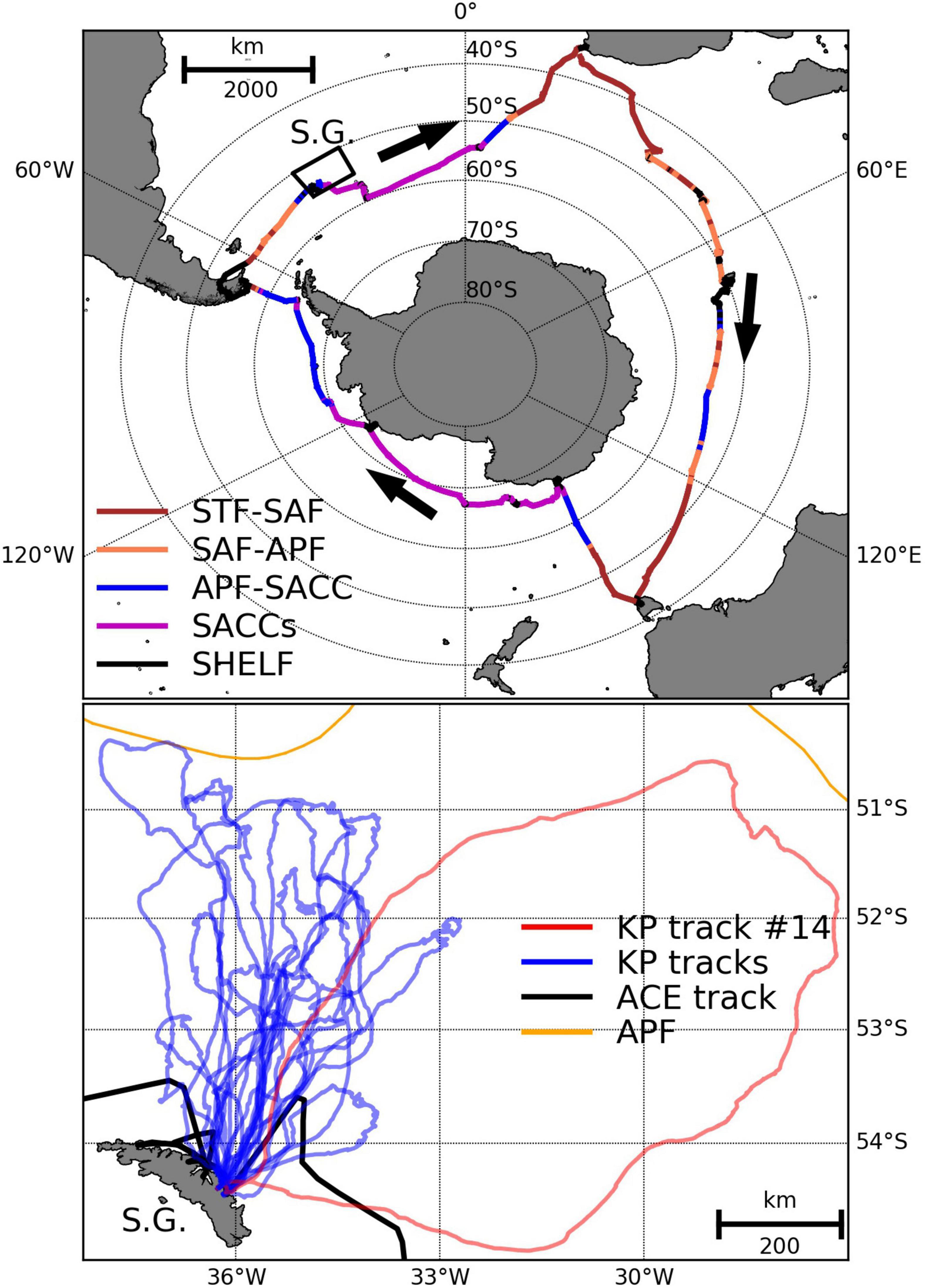
Figure 1. The track of the Antarctic Circumnavigation Expedition (ACE) research vessel (Top) plus GPS positions of the 18 tagged king penguins (Bottom) foraging from Hound Bay. In the top plot, the ACE track is colour coded by interfrontal zone as experienced during the voyage (i.e., fronts are calculated in-situ at a daily time resolution): STF-SAF (sub-Tropical Front to sub-Antarctic Front), SAF-APF (sub-Antarctic Front to Antarctic Polar Front), APF-SACC (Antarctic Polar Front to Southern Antarctic Circumpolar Current Front) and SACCs (Southern Antarctic Circumpolar Current Front to the southern boundary of the Antarctic Circumpolar Current). In the bottom plot, 17 king penguin tracks are shown by blue lines (birds 1–13 and 15–18) and a single red line indicates the anomalous trip of bird 14 that performed a far eastern loop uncharacteristic of birds during the guard breeding stage. The ACE track in the vicinity of South Georgia is indicated by a black line, and the mean position of the Antarctic Polar Front (Orsi et al., 1995) is shown by an orange line. South Georgia (S.G.) is also indicated on both maps.
King Penguins
King penguins breeding at Hound Bay (54°23’S, 36°15’W), South Georgia, were studied between 20th February and the 22nd March 2017. This period coincided with the passage of the ACE voyage past South Georgia (2nd to the 8th March 2017). Only adult chick-rearing king penguins in guard stage were included in this study.
Animal Handling and Instrumentation
A total of 18 individual king penguins were captured as they were leaving on foraging trips. They were instrumented with miniature data-loggers attached to their lower backs with waterproof Tesa® tape and quick-drying two-part epoxy, and marked on their front with permanent black hair dye to aid in reidentification and device recovery (Scheffer et al., 2010). At-sea movements were followed using GPS (Pathtrack nanofix GEO, weight: 32 g; size: 54 × 23 × 17 mm), and dive profiles were recorded using TDRs (G5, CTL, Lowestoft, United Kingdom; weight: 6.5 g; size: 12 × 35.5 mm) recording at 1 Hz. Prey strikes were measured using a tri-axial accelerometer (X8M-3, Gulf Coast Data Concepts, Waveland, MS, United States, weight: 34 g; size: 51 × 25 × 16 mm) recording surge, heave and sway at 25 Hz. Birds were recaptured after one foraging trip and the loggers were retrieved. Battery capacity limited the observation period for both TDR and accelerometer tags. Typically, the accelerometer tags ran out of battery 4–5 days before the penguins returned from foraging at sea.
Foraging Behaviour
Trip characteristics were extracted from GPS data using the ‘trip’ package in R (Sumner et al., 2009) following the application of a speed filter of 14 km h–1 (e.g., Cotté et al., 2007) (which is the fastest observed swim speed of a penguin, see Kooyman and Davis, 1987) to remove any erroneous position estimates (<0.1% of all positions). For each bird, trip duration (days), path length (km), maximum distance from colony (km), and mean and maximum speed (ms–1) were calculated. TDR data were processed using IGOR Pro (WaveMetrics, Version 7, OR, United States) to calculate maximum dive depth; dive duration; number of undulations (also called ‘wiggles’, defined as a depth change rate < 0.25 ms–1); bottom phase duration; and post dive duration (see Ropert-Coudert et al., 2007, for parameter definitions). Depth undulations (wiggles) are indicative of either prey search, prey encounter, predator interaction or other movement, and hence are not a reliable source for detecting prey capture attempts. Shallow travelling dives ≤4 m were excluded (Charrassin and Bost, 2001; Charrassin et al., 2002). For five individuals, the GPS battery expired before completion of the foraging trip so the location of subsequent dives could not be determined.
Prey Encounters
Prey capture attempts were identified using the accelerometry data (e.g., Ropert-Coudert et al., 2006; Zimmer et al., 2011). Vectorial Dynamic Body Acceleration (VDBA), a commonly used proxy of whole body activity (Gleiss et al., 2011), was calculated as:
where Ax, Ay and Az are the dynamic accelerations of the surge, heave and sway axes respectively, calculated by subtracting the static acceleration of each axis (a smooth over 1 s) from the total acceleration (Shepard et al., 2008). There was an upper inflection point at 2.5 m s–2 in the frequency of VDBA across all birds, and this was used as a threshold for diagnosis of prey capture attempts (Supplementary Figure 1), i.e., when VDBA (at 1 Hz) became higher than 2.5 m s–2 during a dive, we inferred that there was a prey encounter and pursuit (Sánchez et al., 2018). This meant that multiple prey encounters (e.g., multiple captures of prey) might be detected as a single prey capture attempt. This was deemed acceptable since our analysis is reliant on the identification of prey encounter dives and prey encounter depths, not the absolute number of prey items (which would require additional sensors, e.g., cameras). For each foraging dive (dives > 4 m) with a prey capture attempt, the depth at which the first VDBA point exceeded 2.5 ms–2 was considered as the prey encounter depth (m). The first 4 m of the descent phase were excluded from the acceleration analysis to be consistent with the dive data and because birds perform strong wing beats at the beginning of a dive to overcome the effects of buoyancy and inertia (Zimmer et al., 2011).
Diet Study
During the same period as the biologging study, 47 faecal samples were collected from other (i.e., not the instrumented birds) king penguins (Le Guen et al., 2020). Ideally, we would have collected samples from the instrumented birds, but due to limited resources and sampling logistics, we were only able to collect samples from birds at the colony whilst the instrumented birds were at sea. Since all the instrumented birds were rearing chicks, only samples taken from chick-rearing birds were considered in this study (16 out of 47 samples collected between 22nd February and 11th March 2017). It is likely that samples were taken from different individuals as they were collected from different nests across the colony (c. 100–150 penguins in total), but it is possible that faeces from the same bird were sampled more than once since adults swap nests regularly. Contamination was minimised during collection by maintaining strict sampling protocols, e.g., sterilising apparatus with ethanol between sampling and only taking samples from the surface of the faecal matter, i.e., not making contact with the underlying soil (for more information, see Le Guen et al., 2020). These data provide vital information on colony-specific diets, which could potentially change seasonally and/or annually in response to changes in prey distributions (e.g., Saunders et al., 2013). Prey taxa for each bird were identified using DNA sequencing (for DNA extraction and sequencing protocols see Supplementary Material).
Echosounder Observations
Echosounder observations were collected continuously along the ACE track (Figure 1) using a Simrad (Bergen, Norway) EK80 echosounder operating a single-beam (10–20 kHz) Wärtsilä ELAC Nautik GmbH (Keil, Germany) LSE179 transducer. Prior to the survey, at-sea trials were conducted to find the optimum settings (i.e., high signal-to-noise ratio) for detection of mesopelagic fish communities: frequency = 12.5 kHz, ping interval = 8 s, power = 150 W, and pulse duration = 16 ms. At this frequency (wavelength c. 12 cm), the majority of the returned signal is expected to originate from large organisms (fish, squid, etc., not zooplankton; Simmonds and MacLennan, 2005), and organisms that possess gas bladders (Proud et al., 2019), e.g., K. anderssoni. An echosounder calibration was conducted at South Georgia using the standard target method (Demer et al., 2015).
Echosounder Data Processing
Raw echosounder data were imported into Echoview version 8 (Myriax, Hobart, Tasmania) and the calibration parameters were applied. Transient noise, impulse spikes and attenuated pings were removed. Data were gridded at a resolution of 5 m depth by 10 km along track, and integrated values (Mean Volume Backscattering Strength, MVBS, dB re 1m–1) were exported to provide data for modelling. Data were also integrated and exported at fine-scale (i.e., 1 ping × 1 m sample) to facilitate comparisons with fine-scale king penguin prey encounters. MVBS values were used to calculate the nautical area scattering coefficient (NASC, average echo intensity per nautical mile squared; m2 nmi–2) and weighted mean depth (WMD, mean depth weighted by linear values of MVBS) values for two depth zones: (1) the penguin foraging zone, between the surface and the depth at which 95% of prey encounters occurred, and (2) the mesopelagic zone, this – by common definition – extended between 200 and 1000 m, and was expected to contain king penguin prey (e.g., myctophids), some of which would have been deeper than the dive range of penguins. At the 12.5 kHz echosounder frequency used, the local WMD value for the mesopelagic zone is essentially equivalent to the mean depth of the principal (strongest) DSL, since during ACE a single broad DSL was observed through most of the expedition. Following the same logic, NASC values calculated between 200 and 1000 m were effectively a proxy for DSL NASC. NASC and WMD values calculated between 200 and 1000 m will be referred to as DSL NASC and DSL depth hereafter.
Predicting Nautical Area Scattering Coefficient and Weighted Mean Depth Using Neural Networks
To model prey availability within the foraging domain of the king penguins at South Georgia (Figure 2), neural networks were built to predict NASC and WMD along the entirety of the ACE voyage track (see Figure 1). Using the entire expedition (as opposed to using a subset of the data close to South Georgia) increased the size of the training set by a factor of 25 and enabled daily and weekly variability (recorded away from the South Georgia foraging site) in prey characteristics to be captured. Environmental variables used as inputs for the neural networks (Table 1) were selected based on previous studies and known relationships between NASC, WMD and the environment (e.g., Klevjer et al., 2016; Aksnes et al., 2017; Proud et al., 2017). To explain diel variation in the depth distribution of biomass resulting from diel vertical migration, sun angle was included as an input variable (see Table 1). All input variables were at the same or higher spatial resolution as the summarised track echosounder observations (10 km), except for sea-level anomaly, which was gridded at a resolution of 0.25° × 0.25°. Values of the input variables were assigned positions along the vessel track using linear interpolation.
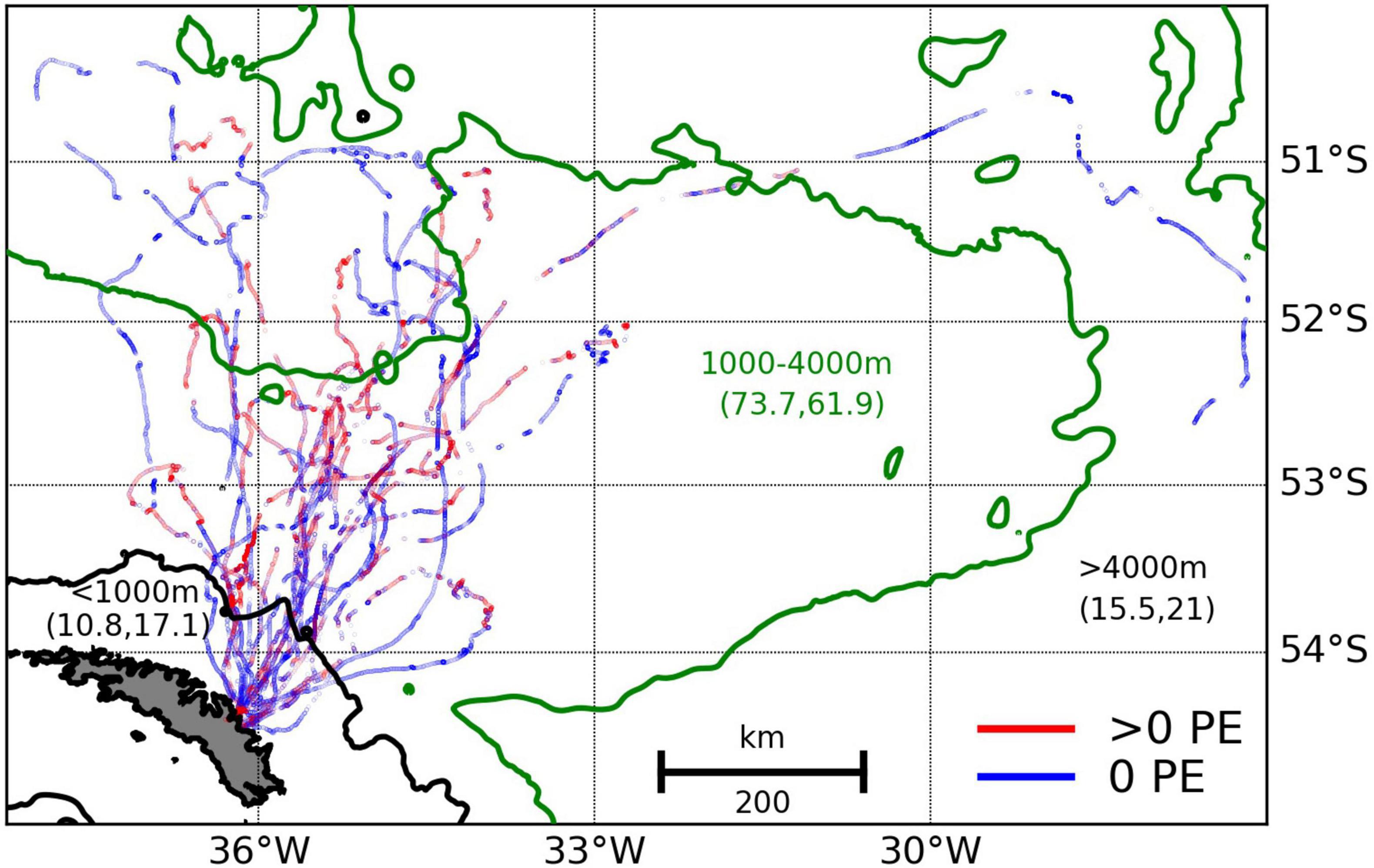
Figure 2. King penguin dive locations (maximum depth > 4 m) where at least one prey encounter (PE) was detected (red points) and where zero prey encounters were detected (blue points). Colour-coded contours split the dives into three depth zones (inshore: <1000 m, and two offshore zones: 1000–4000 m and >4000 m) and the percentage of dives and PEs in each zone is given in parentheses (%dives, %PEs). All dives occur in the Antarctic Polar Front to Southern Antarctic Circumpolar Current Front interfrontal zone. Time-depth recorder loggers and accelerometers ran out of battery for some birds before they returned to South Georgia so not all tracks close.
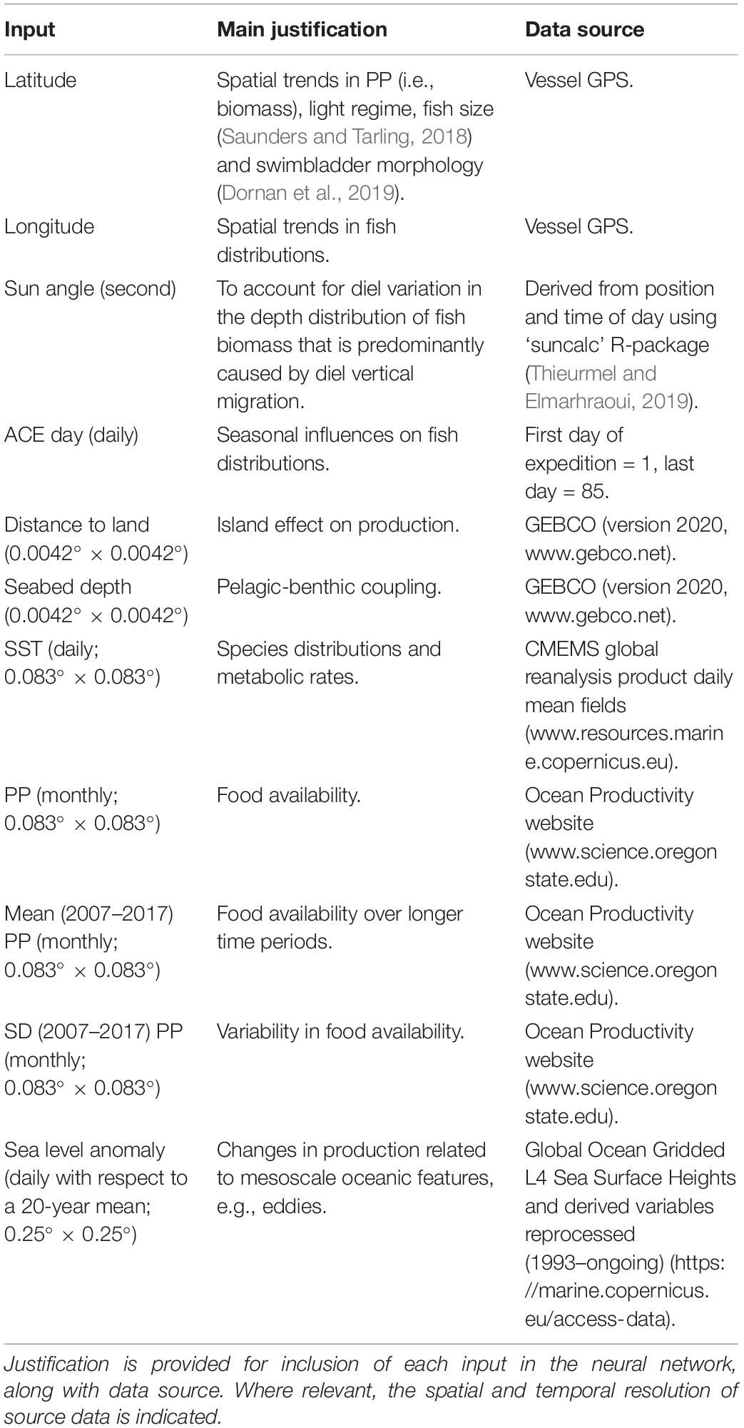
Table 1. Neural network model inputs.
Each 10 km position along the ACE cruise track was classified as belonging to one of four interfrontal zones (Figure 1) evident in vertical potential temperature profiles. Daily mean potential temperature data at 25 m depth intervals from 100 m to 300 m depths were extracted from the Global coupled FOAM quarter degree model run by the United Kingdom Met office1 along the ACE track for each day of the cruise. Each ship location was then associated with a interfrontal zone based on the potential temperatures at 200, 300, and 500 m (Figure 1) evident in previous work (e.g., Orsi et al., 1995; Belkin and Gordon, 1996; Boehme et al., 2008). All locations associated with a water depth of less than 1000 m were classified as being on the shelf.
Neural network inputs (Table 1) and outputs (NASC and WMD calculated over the penguin foraging zone and mesopelagic zone) were scaled to between 0.0001 and 0.9999 (weighting the contribution of each input equally). Temporal inputs were predominantly at daily resolution apart from PP (see Table 1), which was monthly and hence values for February and March were assigned to penguin dive locations over the study period. R-packages ‘caret’ (Kuhn, 2008, 2020) and ‘nnet’ (Venables and Ripley, 2002) were used to train and test the neural networks (10-fold cross validation; 80%/20% split for train/test data, respectively). A standard 3-layer setup (input, hidden layer, output) was used. The number of nodes in the hidden layer (6–30 nodes) and decay parameter (regularization parameter to avoid over-fitting: 0.001–0.1) varied, and optimum models were selected based on validation set mean root-mean-square error (RMSE) values (mean over the 10 folds).
Penguin Habitat Selection Modelling
We did not have direct echosounder observations at penguin dive locations, so took a modelling approach to infer the likely prey-field characteristics at dive sites on specific days during the study period. This was made possible by including ACE day (see Table 1) in the NASC and WMD models to capture daily and weekly variability; note that we used ACE day rather than day of year to avoid forcing the model to weight day 1 (January 1st) and day 365 (December 31st) very differently, when in fact these 2 days should be weighted similarly since they are only 1 day apart. Daytime king penguin dive data that could be associated with valid GPS locations were used to study king penguin habitat use. Bird 14 was excluded from this analysis due to anomalous behaviour (see trip with far eastern loop in Figure 1), which was not consistent with other studies for birds in this stage (Scheffer et al., 2012), and also because its TDR logger ran out of battery (note absence of eastern loop in Figure 2). Habitat selection models (e.g., Aarts et al., 2008) were used to define the pelagic foraging habitat suitability of the king penguins. The outer limit of available habitat was set conservatively (to limit spatial extent of sampling domain, see Hazen et al., 2021) as a circle with a radius of 1.1× the maximum foraging range from the Hound Bay king penguin colony (Wakefield et al., 2017). Dives where the seabed was <600 m (the expected maximum depth of DSLs in this region) were excluded from this analysis and hence habitat suitability in this context refers to pelagic dives as opposed to shallow inshore/benthic dives (where we did not have acoustic observations). Dive locations were assigned values of the environmental variables (see Table 1) at the same scale as the modelled NASC and WMD observations. Environmental variables were averaged over an area demarked by a circle (diameter = 10 km) centred on each dive location. Predicted NASC and WMD, distance to colony and seabed depth were extracted for each dive (presence) location and day (Figure 2) as well as for three randomly chosen pseudo-absence locations (three points drawn from the entire accessible geographic area) for every dive location to represent habitat availability (Aarts et al., 2008). Binomial generalised additive models (GAM; logit link function) with presence/pseudo-absence location as the response, and the prey indices (predicted NASC and WMD), seabed depth and distance to colony as explanatory variables were fitted using the R package ‘mgcv’ (Wood, 2006). Models were fitted using interactions between related covariates (using tensor smooths; Wood, 2006), e.g., an interaction between seabed depth and distance to colony is expected to influence habitat suitability since birds only utilise shallow water when close to the colony; note that some degree of correlation is expected between seabed and distance to colony. GAMs were parameterised using full tensor product smooth terms: (te1) distance to colony * seabed depth; (te2) NASC50–260 m * WMD50–260 m, representing the penguin ‘prey’ component, and (te3) NASC200–1000 m * WMD200–1000 m representing the ‘DSL’ component (i.e., addressing the question does the depth and intensity of DSLs influence diving behaviour?).
For each model, the random pseudo-absence selection was repeated 30 times, resulting in 30 model iterations. Model selection was conducted using Akaike Information Criterion (AIC), cross validation and Area Under the Receiver Operating Curves (AUC), which are conservative and permit violation of model assumptions relating to non-independence of errors that are inherent in tracking data (spatial and temporal autocorrelation). Three candidate models were compared using AUC: (1) the null model (te1), (2) the ‘prey’ model (te1+te2), and (3) the ‘prey+DSL’ model (te1+te2+te3). Selected GAMs were then averaged over the 30 iterations using the ‘MuMIn’ R package (Barton, 2020) and used to predict habitat use probabilities around the Hound Bay colony. Since predictions of NASC and WMD will have an associated error (RMSE from neural networks), uncertainty associated with the habitat model will be biased low.
Results
In total, 18 birds were tracked, and faecal samples were collected from 16 non-instrumented birds. Bird 14 was excluded from dive analysis due to anomalous foraging behaviour that was not consistent with previous studies, and no accelerometer data were collected from bird 16 due to a tag malfunction.
King Penguin Foraging Trip Characteristics
All king penguin foraging trips headed north from South Georgia in the direction of, but never reaching, the Antarctic Polar Front. The birds remained in the APF-SACC interfrontal zone during guard stage (consistent with other studies; see Scheffer et al., 2012). Foraging trips took place between 20th February and 22nd March and had an average duration of 10.2 days (range = 4.8 to 17.8 days; 183.8 days total), path length of 820.7 km (range = 293.9 to 1837.2 km) and mean maximum distance from colony of 317.2 km (101.7 to 672.8 km). Specific details of individual trips are given in Supplementary Table 1.
A total of 37,275 dives deeper than 4 m were identified during 165.3 days of total tracking time across all birds between February 20th and March 20th (using TDR tags; see Figure 2 and Supplementary Table 2). On average, birds dove 228 times per day and each dive included 8.2 undulations/wiggles (i.e., potential prey encounters). The maximum dive depth recorded was 352 m and the maximum dive duration was 9 min 10 s. Birds dived mostly during the day (c. 73% by dive duration), with depths increasing progressively after sunrise and reduced around sunset (Supplementary Figure 2) in keeping with both diel vertical migration (DVM) of prey and increased visibility with depth as sun angle increases (Bost et al., 2002; Pütz and Cherel, 2005).
King Penguin Prey Encounters and Pelagic Vertical Habitat Use
A total of 45,958 (43,063 with valid GPS locations) prey encounters deeper than 4 m were detected during 99.3 days of total tracking time across all birds between February 20th and March 16th (using accelerometer tags; see Figure 2 and Supplementary Table 3). On average there were 462.8 prey encounters per day and hence around 2 prey encounters per dive (i.e., 462.8 prey encounters per day/228 dives per day). The average prey-encounter depth was 107.1 m (lower quartile = 67.1 m; upper quartile = 174.8 m), and 95% of encounters occurred at a depth ≤260 m, which was used to define the lower boundary of the king penguin foraging zone (see sections “Predicting Fish Distributions Using Neural Networks”, “King Penguin Habitat”, and “King Penguin Habitat Suitability”): very few prey encounters occurred deeper, so including acoustic backscatter from beyond this depth as ‘prey’ would have resulted in inclusion of features (such as DSLs occurring deeper than 260 m) that were not typically accessed by king penguins. The vast majority of the birds’ foraging effort was off shelf (seabed > 1000 m; 38,394 out of 43,063 prey encounters were offshore). We thus compared the vertical distribution of prey encounters offshore to offshore echosounder observations (seabed > 1000 m; c. 465 km of vessel track) made in the same interfrontal zone (APF-SACC; see Figure 1) between 4th March and the 18th March 2017. Echosounder observations recorded in the top 50 m were excluded due to surface noise. We compared day (29,877 prey encounters; see Figure 3A) and night (8,517 prey encounters; see Figure 3B) separately to avoid complications associated with prey DVM. MVBS was plotted for each depth interval (0–600 m by 10 m intervals) and MVBS level (−80 to −40 dB re 1m–1 by 3 dB re 1m–1 intervals) e.g., the cell in the bottom left-hand corner of Figures 3A,D is the MVBS value calculated by first thresholding the data by the MVBS level (−80 to −77 dB re 1m–1) and then integrating the remaining observed echo intensity over the depth interval (590 to 600 m).
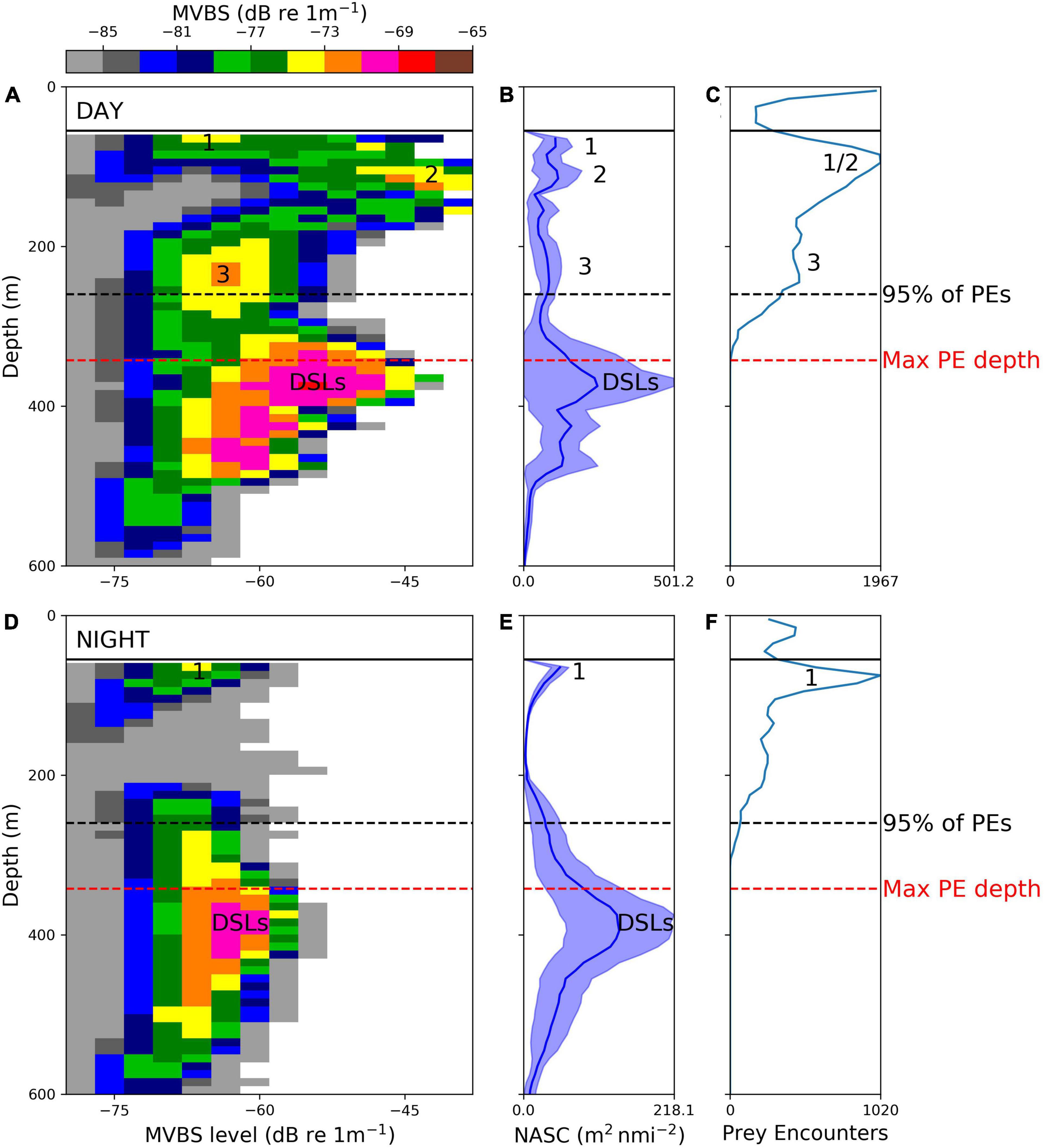
Figure 3. Offshore (seabed depth > 1000 m) king penguin prey encounters (PEs) detected between 20th February and 16th March 2017 and acoustic observations of water-column backscattering intensity distribution in the Atlantic sector of the Southern Ocean (Antarctic Polar Front to Southern Antarctic Circumpolar Current Front interfrontal zone; 4th March to 18th March 2017). Panels (A,D) show observed mean volume backscattering strength (MVBS, –80 to –65 dB re 1m–1) by depth interval (0 to 600 m in 10 m intervals) and MVBS level (–80 to –40 dB re 1m–1 in 3 dB re 1m–1 intervals) during day and night, respectively. Panels (B,E) show MVBS collapsed into 1D mean nautical-area scattering coefficient (NASC) values, integrated over 10 m intervals between 50 and 600 m (echosounder observations recorded in the top 50 m were excluded from analysis due to surface noise), blue shading represents variability (95% confidence intervals) in calculated NASC values (standardised into 1 km along-track segments). Panels (C,F) show numbers of prey encounters by 10 m depth intervals from 0 to 600 m. Numbers indicate different prey types (1 = low intensity schools, 2 = high intensity schools, and 3 = clusters of schools termed ‘prey patches’; see section “Acoustically Detected Prey Field” for more information). Deep scattering layers (DSLs) were labelled where values of MVBS peaked in the mesopelagic zone. 95% of all prey encounters occurred shallower than 260 m (black dashed line). Red dashed line is the maximum depth of all recorded prey encounters.
Acoustically Detected Prey Field
DSLs, which were ubiquitous throughout the APF-SACC interfrontal zone, were the source of most of the recorded echo energy (78.3% during the day and 92.4% during the night; note that the top 50 m was excluded) but even at night these DSLs appear to be deeper than the dive capability of the king penguins (Figure 3). Fish schools (isolated echogram features, 10s of m in width and height) occurred ephemerally in the epipelagic zone, observed at both low echo intensity (prey type 1: MVBS level = −70 to −65 dB re 1m–1; see Figure 3A) and high echo intensity (prey type 2: MVBS level = −50 to −40 dB re 1m–1; see Figure 3A). The differences in MVBS level imply that prey types 1 and 2 differ in numerical fish density, target strength or both. A third prey type, which we termed ‘prey patches’ (Béhagle et al., 2017) (prey type 3: MVBS level = −70 to −60 dB re 1m–1; see Figure 3A), comprised clusters of linked schools (see Supplementary Figure 3) that, due to echosounder beam geometry, would appear as layers if they were observed deeper in the water-column (the echosounder beam broadens with depth and hence sampled volume increases with depth, reducing horizontal resolution and blurring the boundaries between discrete prey structures giving them a continuous appearance). The vertical distributions of prey types 2 and 3 shifted markedly between day and night (see Figures 3A,D) and hence were likely composed of species that performed DVM. The modal depth in daytime penguin prey encounters matched with the modal depth of prey type 2 (high energy fish schools) NASC (Figure 3). Prey type 1 was persistent throughout the daily cycle and matched with peaks in penguin prey encounters both during the day and night (Figure 3).
Diet Analysis
Only 9 of the 16 chick-rearing penguin faecal samples returned useful DNA data (likely due to degradation of the DNA in the gut during digestion). Of these, eight contained DNA of eight species of fish (Table 2) but only two contained euphausiid crustacean DNA (Euphausia superba and Thysanoessa macrura). Fish also eat krill and so it is possible that presence of krill DNA in penguin faecal samples is a consequence of secondary ingestion. Higher occurrences of krill were found in the other breeding stages (3 out of 16 samples for incubating birds, and 5 out of 16 samples for non-breeding birds). No prey species were encountered in the procedural blanks, thus it is likely that no contamination occurred during the DNA extraction phase.
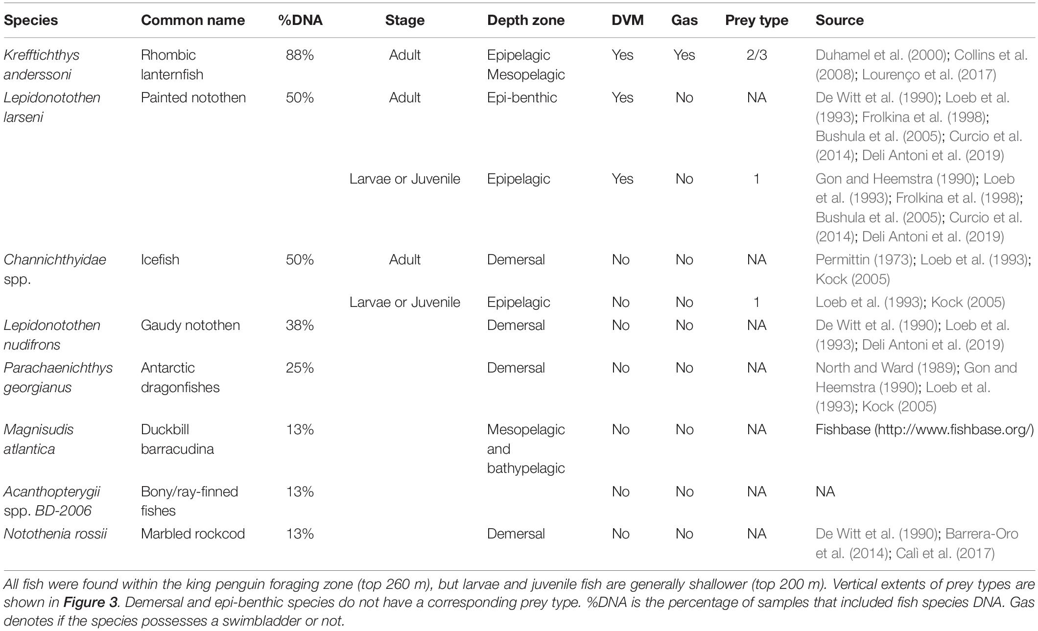
Table 2. Fish species detected in king penguin (chick rearing stage = 8 penguins) DNA faecal samples.
Consideration of the known DVM behaviour, biology, and depth distribution of these fish species (Table 2) links them to the three prey types observed (see section “Acoustically Detected Prey Field” and Figure 3). Both adult icefish (Channichthyidae spp.) and painted notothen (Lepidonotothen larseni) are associated with the seabed so probably do not make up a large percentage of the penguins’ diets (90% of prey encounters are pelagic; these fish may be taken opportunistically at the start or end of trips). However, larvae and juveniles of these species occur within the epipelagic zone and since they are without gas-filled swimbladders are relatively weak scatterers, which matches with prey type 1 (icefish also do not perform DVM, which is consistent with the observed DVM pattern). The other two prey types (2 and 3) likely correspond to rhombic lanternfish (K. anderssoni), since they are known to perform DVM, have gas-filled swimbladders (i.e., high intensity acoustic targets) and occur in both the epipelagic and mesopelagic zone.
Predicting Fish Distributions Using Neural Networks
NASC and WMD were calculated for the penguin foraging zone (50–260 m; defined in Figure 3) and the mesopelagic zone (200–1000 m), resulting in four model outputs (NASC and WMD for both depth zones) and hence four neural networks. Models were trained using 80% of the ACE echosounder data (n = 1,636 samples), and model selection and evaluation was based on validation set (n = 164 × 10 folds) and test set (n = 409 samples) RMSE, respectively. Optimum networks for each of the outputs were as follows (see Figure 4): (A) NASC50–260 m, nodes = 22, decay = 0.001 (test RMSE = 295.6 m2 nmi–2; R2 = 0.66); (B) NASC200–1000 m, nodes = 30, decay = 0.001 (test RMSE = 289.9 m2 nmi–2; R2 = 0.81); (C) WMD50–260 m, nodes = 28, decay = 0.001 (test RMSE = 18.4 m; R2 = 0.73), and (D) WMD200–1000 m, nodes = 28, decay = 0.001 (test RMSE = 47.8 m; R2 = 0.75).
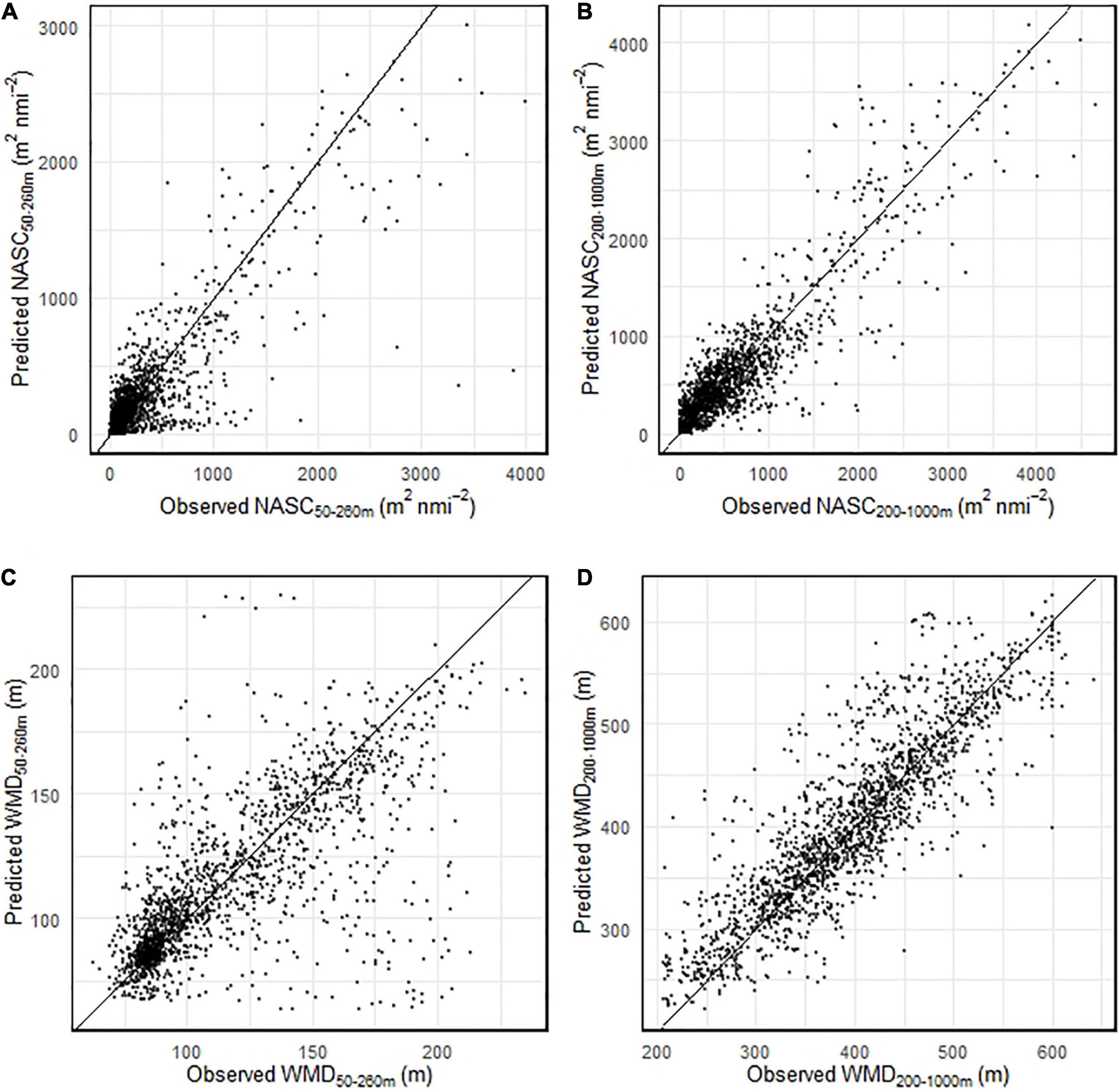
Figure 4. Neural network predictions of nautical-area scattering coefficient (NASC; A,B) and weighted-mean depth (WMD; C,D) versus observations averaged over 10 km along track intervals collected during the Antarctic Circumnavigation Expedition.
King Penguin Habitat
Predicted gridded NASC and WMD daily values (sun angle was set to the local daily maximum value) were averaged over the king penguin foraging period and plotted (Figure 5; standard deviation plotted in Supplementary Figure 4). Mean areal values of NASC50–260 m and NASC200–1000 m over the penguin foraging domain were c. 322 and 335 m2 nmi–2, respectively. Mean areal values of WMD50–260 m and WMD200–1000 m over the penguin foraging domain were c. 78 and 336 m, respectively. King penguin dive locations were associated with shallow prey (Figure 5C) that had high NASC values (Figure 5A) in their foraging zone (top 260 m), and with relatively shallow (Figure 5D) and high intensity DSLs (Figure 5B) in the 200–1000 m depth range. NASC and WMD were also predicted for the region surrounding the Kerguelen Islands (see Supplementary Figure 5), which is also home to colonies of breeding king penguins. Spatial patterns of prey were very different between the two regions: in the Kerguelen region, mean NASC200–1000 m was much higher (c. 1599 m2 nmi–2), mean NASC50–260 m was much lower (c. 132 m2 nmi–2), and DSLs were substantially deeper (c. 487 m; a depth far beyond the diving capabilities of king penguins).
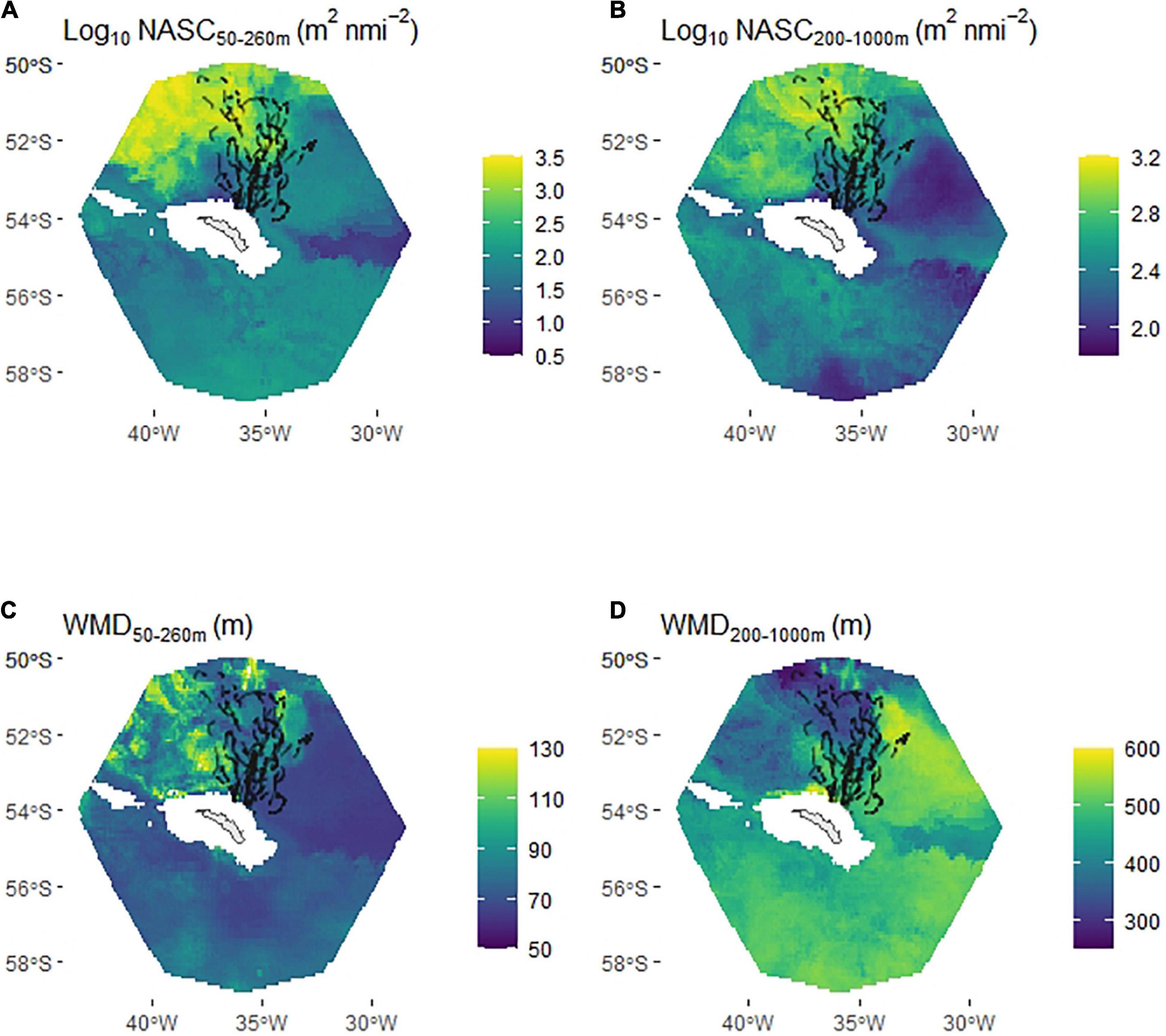
Figure 5. Predicted mean (daily values averaged between 20th February and 18th March 2017) daytime nautical-area scattering coefficient (NASC; A,B) and weighted-mean depth (WMD; C,D) values for 17 (bird 14 excluded) chick-rearing king penguins foraging from South Georgia. Foraging domain defined as 1.1× max foraging range = 508.1 km. Grid cells that had a seabed <600 m were excluded. All penguin dive locations (with and without prey encounters) shown by black points.
King Penguin Habitat Suitability
Excluding Bird 14 (see section “Materials and Methods”) left a total of 19,504 dives (out of 23,646 daytime dives and 37,254 in total) available for the habitat selection models. The ‘prey+DSL’ model had significantly better support than the null and prey models (Figure 6C) and a substantially lower AIC value (mean over the 30 model runs was 18,472 compared with mean values of 21,226 and 30,717 for the prey and null models, respectively, indicating that the more complex prey-based models were not being overfit). The ‘prey+DSL’ model was used to predict mean habitat suitability over the period (Figure 6D); note that NASC values are integrated over the penguin foraging zone and the mesopelagic zone in these models and hence are much larger than the values in Figure 3, which are integrated over 10 m depth intervals.
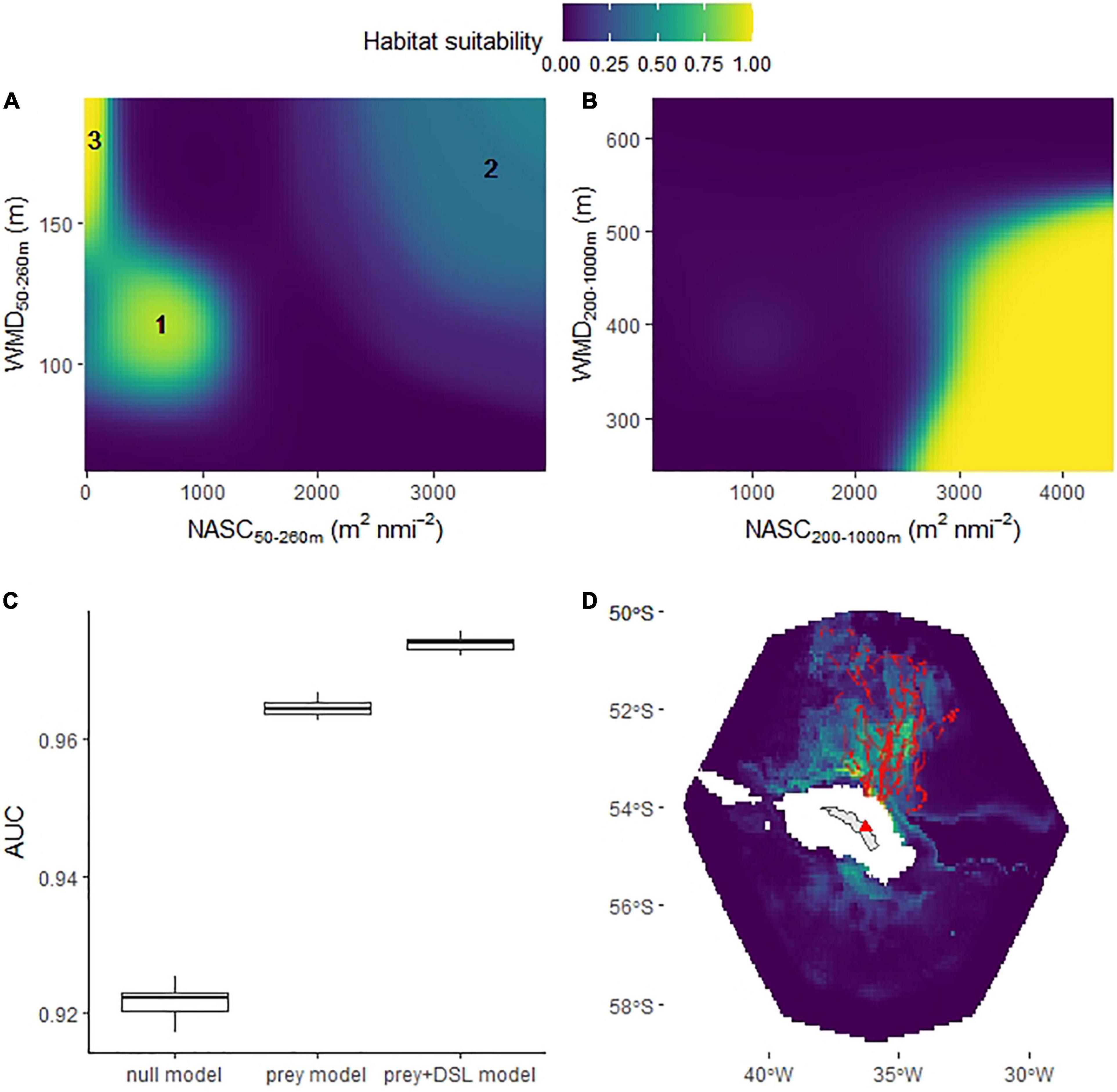
Figure 6. Habitat suitability (based on daytime dive locations) of chick-rearing king penguins foraging from South Georgia. Partial plots (averaged over 30 model iterations) show additive effect on habitat suitability by tensor product terms relating to king penguin prey (nautical-area scattering coefficient/weighted-mean depth 50–260 m) (A) and deep scattering layers (DSLs) (nautical-area scattering coefficient/weighted-mean depth 200–1000 m) (B). Model selection was based on Area Under the Curve (AUC) (C), box plot shows AUC results for 30 model runs, where each run comprised a random selection of pseudo-absences. The best supported model (‘prey+DSL’ model), averaged across the 30 model runs, was used to map mean habitat suitability between February 20th and March 18th (D). Prey types (1, 2 and 3), defined in Figure 3 and Table 2, were related to patterns in the king penguin prey component of the habitat suitability model (A). Red points are penguin dive locations and red triangle marks the location of the colony.
King penguin habitat suitability declined with distance from the colony, and since we used the distance to colony * seabed depth interaction (te1), shallow seabed depths tended to be used close to the colony but were avoided as distance from it increased. Habitat suitability increased in the presence of high intensity and relatively shallow DSLs (Figure 6B). Three distinct features were evident in the partial plot for the prey component of the GAM (te2; Figure 6A) that were related to the three prey types defined in Figure 3 (based on WMD and NASC) and Table 2 (based on diet studies).
Discussion
Our results indicate that king penguins in guard stage at South Georgia do not feed directly on the ubiquitous DSLs around their colony, as these were found to be outside their diving range during the study period. Instead, they likely target smaller, ephemeral schools occurring above the DSLs. This offers strong support for the idea that availability and prey type (or quality), rather than abundance per se influences predator–prey interactions at fine (10s of m) vertical scales (e.g., Benoit-Bird et al., 2013; Boyd et al., 2015). The link between targeted fish schools and the inaccessible DSLs, which is evident at a 10 km horizontal scale, may be related to ontogeny (e.g., juveniles forming clusters of shallower aggregates) or other food web links (e.g., changes in depth distribution related to species, size, DVM, or environmental conditions, e.g., light). However, these findings are based on a single site, breeding stage and year and warrant further investigation.
Study Caveats, Considerations, and Recommendations for Future Work
The approach taken here provides the foundations of a framework to tackle an important problem in marine ecology – linking at-sea diving predator distributions with their prey across multiple spatial and temporal scales – using a combination of acoustics, diet studies, animal tracking and modelling. Such a comprehensive and multi-faceted approach naturally incurs limitations, which will ultimately need to be addressed in future studies. For example, there was poor spatial overlap between penguin dive locations and the vessel track. Use of a single echosounder frequency did not enable target identification. However, since the frequency used was relatively low (12.5 kHz), most of the received backscattering intensity could be attributed to fish. Due to surface noise, we were not able to make observations in the top 50 m and hence some schools at the surface may have been missed. This may explain why the shallow zone neural networks systematically underestimated NASC and WMD (see Figure 4). In future studies, structured and statistically robust (see Jolly and Hampton, 1990) multifrequency/broadband acoustic surveys with coincident trawling in known (or predicted) penguin foraging grounds should be conducted to enable prey species identification and provide information on prey size distribution.
We compared penguin prey encounters with predicted NASC values to study predator–prey interactions. However, not all predicted encounters will be a result of prey interactions since prey and predator encounter discrimination is not possible using accelerometery data alone, but the number of predation events is expected to be relatively low. We also used a neural network to predict prey characteristics because relationships between acoustic target strength and the environment are known to be non-linear and complex (e.g., see Jech et al., 2015). Neural networks provided very good predictive power but are hard to interpret, precluding any discussion related to the importance of the correlated model inputs.
Spatially resolved ecosystem based management requires information on predator and prey distributions and on the interactions between them. We used model-predicted physical and biological variables to model prey NASC and WMD, which were then used to model predator habitat suitability. Instead of this multi-model approach, a single model based on the environmental covariates could have been used to predict habitat suitability. Whilst this less complex approach would ultimately be more statistically robust, it would not provide the means to determine the importance of the vertical distribution of different prey structures (e.g., scattering layers and schools) in predicting habitat suitability (i.e., providing information on predator–prey interactions). In the absence of coincident prey observations, future modelling work should test the utility of our multi-model approach by comparing predictions with output from simpler models that only consider environmental observations.
We also modelled (binomial GLM) prey encounter dives (=1) versus non-prey encounter dives (=0) using the habitat suitability model predictors (analysis not presented) but did not find good agreement between the data and the models. This suggests that the data we used (predicted NASC and WMD values) do not explain the variance in prey capture well, which is likely to be better explained by environmental covariates that contribute to successful prey capture, e.g., surface illumination and light attenuation in the water-column (not available in this study).
King Penguin Prey
King penguins from South Georgia likely fed on barracudina close to the seabed and juvenile icefish and painted noties, that typically occupy reefs and kelp beds in the coastal region, on their return trips to the colony (Frolkina et al., 1998). Although relatively infrequent, occurring in just 13% of faecal samples that contained fish DNA from individual chick-rearing penguins, barracudina may make up a relatively large proportion of king penguin diet by mass due to their large size (Olsson and North, 1997). In offshore regions, where the majority of foraging takes place, penguins targeted specific prey types (isolated and larger-scale patches of fish schools, comprised of various species across different life-history stages and depth ranges) within their diving range. Given that king penguins typically require c. 2.3 kg/day of fish (Bost et al., 1997; Putz et al., 1998), our results indicate that penguins must have on average obtained around 10.1 g of prey per dive or 5 g per prey encounter. Since adult K. anderssoni (main prey item of chick rearing penguins) weigh around 4 g at maximum standard length (c. 7 cm) (see Saunders et al., 2020), this would suggest that on average each prey encounter included capture of >1 fish. Penguins likely focused on juvenile (since they do not eat larvae, see Ratcliffe and Trathan, 2011) fish species during the daytime that occurred in the mid-to-upper epipelagic zone (e.g., painted noties/icefish), but also probably fed on adult K. anderssoni both during the day and at dawn/dusk during fish vertical migration. Increases in shallow epipelagic prey density were related to relatively shallow and dense (high echo energy) DSLs, which is in agreement with the findings of Fielding et al. (2012) that acoustic backscattering intensity was positively related to the number of fish schools. This association can be explained by the strong coupling, via DVM and ontogenesis, between highly dynamic shallow water biomass (in the form of ephemeral schools and larvae/juveniles) and mesopelagic biomass (Pinti et al., 2021).
Electrona carlsbergi and K. anderssoni are known to be the dominant schooling myctophid species close to South Georgia, and occur at depth of between 60 and 300 m (Saunders et al., 2013). King penguin chick rearing success has been found to increase when K. anderssoni form a large component of their diet (Olsson and North, 1997). We found that 88% of the chick-rearing birds had K. anderssoni in their diet, whereas no E. carlsbergi were found. Saunders et al. (2013) reported that E. carlsbergi, which are typically located in water associated with the Antarctic Polar Front (Hulley, 1981; Zasel’sliy et al., 1985; Saunders et al., 2014), were absent or in low abundance in some years, whereas K. anderssoni occurred more regularly every year. Since king penguins in guard stage do not feed at the Antarctic Polar Front, the absence of E. carlsbergi in the diets of birds in this study is likely to be a consequence of the constraints on foraging ranges during the guard stage of the breeding season (Olsson and North, 1997), but it is also possible that E. carlsbergi were consumed but not detected due to the relatively low sample size in our diet study.
Layers and associated patches of swimbladdered fish have been observed during the daytime in the Scotia Sea (Saunders et al., 2015; Lourenço et al., 2017) and at Kerguelen (Béhagle et al., 2017). Prey patches at Kerguelen, which were observed shallower than 180 m, were likely comprised of K. anderssoni and Protomyctophum spp. and disappeared at night owing to DVM (as observed here). The depth range of K. anderssoni around Kerguelen is between 100 and 150 m (Bost et al., 2002; Charrassin et al., 2004) and overlaps with the depth range of prey type 2 identified in this study, classified as K. anderssoni through diet analysis. This prey type may also include Protomyctophum spp., since Protomyctophum choriodon have been commonly found in king penguin diets, particularly during February and March (Olsson and North, 1997). Therefore, foraging behaviour of king penguins at South Georgia appears similar to that found at Kerguelen as is the apparent association between targeted prey patches and DSLs.
Predator–Prey Interactions
We found good agreement between the vertical distribution of acoustically detected fish schools and that of king penguin prey encounters at fine vertical scales (10s of m), and were able to map king penguin foraging habitat based on predicted 3D prey distributions at local horizontal scales (10 km) after controlling for regional-scale (10s–100s km) effects related to distance to colony and bathymetry. Within the habitat available to king penguins, defined to be 1.1× maximum foraging range from their colony, prey resources (full water-column NASC) were found to be relatively low when compared to other similar sites (e.g., Kerguelen, see Supplementary Figure 5). King penguins concentrated their diving effort in an area with relatively high levels of predicted NASC toward (but not reaching) the Antarctic Polar Front, likely containing relatively high densities of prey. Vlietstra (2005) found that in a similar resource-limited environment, fine-scale overlap of seabird and prey distributions increased when compared to resource-rich environments. Since prey distributions can shift significantly both seasonally and annually, e.g., presence/absence of E. carlsbergi around South Georgia (Saunders et al., 2013), potential king penguin foraging habitat may change from being a resource-limited to a resource-rich environment. However, previous work has shown that king penguins have foraged in a similar area (Scheffer et al., 2010), suggesting that it may be characteriesd by predictability of resources and low variation in prey availability. It follows that the more constrained predators are by their environment (i.e., the harder it is to find prey compared with random search) the more tightly coupled the relationship between prey and predators will be. Perhaps the most important foraging constraint for king penguins is vertical accessibility, and studies of seabirds in the Humboldt Current have found that this is more important in predicting seabird foraging habitat selection than prey density throughout the water column (Boyd et al., 2015). It is perhaps no coincidence that DSL depth coincides with the maximum dive depth of king penguins: myctophids may go to these depths to reduce predation risk, as opposed to tracking isolumes (Røstad et al., 2016) or being physiologically constrained by swimbladder function (Bone et al., 1995). A relatively small shallowing of DSLs (10s of m), which is predicted by 2100 (Proud et al., 2017), could open up a very large resource to king penguins that is perhaps more reliable than the presently targeted ephemeral fish schools close to the surface. This would of course reduce prey variance at fine and local scales and make it very difficult to predict predator distributions (Logerwell et al., 1998), i.e., the spatio-temporal relationship between predator and prey would weaken as there would be a large number of areas with an abundance of food but no penguins. Under this scenario, availability of prey to king penguins would become analagous to present prey availability to elephant seals now: the very deep diving capability of elephant seals gives them access to the entire mesopelagic zone and the DSLs there, and so it is very difficult to predict elephant seal dive locations from modelled prey distribution patterns because prey is, to an extent, ubiquitous (McMahon et al., 2019). The degree to which DSLs become shallower around South Georgia in the future will depend on whether their depth is driven by environmental conditions (e.g., light) or predation risk – if the latter, they might not change.
Implications for Marine Spatial Planning and Conservation Management
Protection of key Southern Ocean predators and prey is becoming increasingly important as fishing of lower trophic levels (e.g., squid and toothfish; Agnew et al., 2005; Kock et al., 2007) continues and other fisheries expand (e.g., Antarctic krill; Nicol et al., 2012). In this study, we have linked high intensity (and likely high biomass) DSLs with penguin habitat suitability. Penguins are likely drawn to these locations to feed on DSL-associated schools that occur within their dive range. This result supports the approach taken by Hindell et al. (2020) for defining AESs, which assumes that predator aggregations are indicative of elevated productivity and biomass at lower trophic levels. Since DSL intensity is readily predictable at local scales, conservation management could use modelled DSL intensity as a proxy for important predator foraging grounds to designate AESs. However, strong correlation between predators and lower-trophic level biomass is not ubiquitous (Boyd et al., 2015), and is likely to vary by species, season, access to habitat and prey distribution. Similarly, drivers of prey abundance are not always good predictors of predator distribution patterns, particularly in anthropogenically altered environments (Grémillet et al., 2008; Sherley et al., 2017). Therefore, it may not be prudent to define AESs over large areas based on ocean basin scale correlations. Instead, a regional approach, which considers seasonal variations in local populations (e.g., changes in predator distribution due to breeding stages, etc.), might provide a more informed basis for designating MPAs: the habitat suitability model developed in this study could be used to identify AESs within and beyond the SGSSI MPA (see Warwick-Evans et al., 2018; Handley et al., 2020).
Data Availability Statement
The datasets presented in this study can be found in online repositories. The names of the repository/repositories and accession number(s) can be found at: https://zenodo.org/rec ord/3587678#.YPArB-hKiF4 and https://doi.org/10.17630/d92c1af3-6149-4bb5-aa14-6fb00ef3a85a for the acoustic and penguin tracking data respectively.
Ethics Statement
The animal study was reviewed and approved by the Government of South Georgia and the South Sandwich Islands (regulated activity permit number 2016/048), the British Antarctic Survey and the University of St Andrews.
Author Contributions
RP collected the echosounder data, wrote the manuscript, and performed data analysis. CLG collected the echosounder data and king penguin data, performed preliminary analysis of king penguin and echosounder data, and produced a thesis chapter relating to the study. RBS collected the penguin data and contributed to writing the manuscript. AK helped with the accelerometery data analysis and contributed to writing the manuscript. YR-C provided guidance on data analysis methods and contributed to writing the manuscript. NR conceived the habitat preference analysis and contributed to writing the manuscript. SJ performed the DNA sequencing. AW performed the DNA extraction and contributed to writing the manuscript. JPYA provided the accelerometery tags and contributed to writing the manuscript. RAS provided literature information on diet study species and contributed to writing the manuscript. PGF collected echosounder data, performed the calibration at South Georgia, and contributed to writing the manuscript. LB assigned frontal zones to track positions and contributed to writing the manuscript. ASB conceived the study, planned the field activities and contributed to writing the manuscript. All authors contributed to the article and approved the submitted version.
Funding
The at-sea data collection and 50% of CLG’s Ph.D. studentship was provided by the Swiss Polar Institute as a grant ‘Unlocking the Secrets of the False Bottom’ to ASB. The School of Biology, University of St Andrews, funded the other 50% of CLG’s studentship. Work at South Georgia was supported by the Natural Environment Research Council’s Collaborative Antarctic Science Scheme (CASS-129), a grant from the Trans-Antarctic Association grant to RBS, and a British Antarctic Survey Collaborative Gearing Scheme grant to RBS and ASB. ASB and RP were supported in part by UKRI/NERC under grant NE/R012679/1.
Conflict of Interest
The authors declare that the research was conducted in the absence of any commercial or financial relationships that could be construed as a potential conflict of interest.
Publisher’s Note
All claims expressed in this article are solely those of the authors and do not necessarily represent those of their affiliated organizations, or those of the publisher, the editors and the reviewers. Any product that may be evaluated in this article, or claim that may be made by its manufacturer, is not guaranteed or endorsed by the publisher.
Acknowledgments
We thank the staff at the British Antarctic Survey base at King Edward Point (South Georgia), Quark Expeditions and the crew and staff of the Ocean Endeavour and the FPV Pharos South Georgia for their help with the fieldwork logistics. We also thank the Swiss Polar Institute and the ACE foundation for funding our ACE project, and all our colleagues who assisted with acoustic data collection at sea: Matteo Bernasconi, Inigo Everson, and Joshua Lawrence. We thank Yves Cherel for fruitful discussion on the role of prey patches for king penguins in the Kerguelen region. We also thank C. Ribout and the Centre for Biological Studies of Chizé for conducting the sexing analyses of the birds.
Supplementary Material
The Supplementary Material for this article can be found online at: https://www.frontiersin.org/articles/10.3389/fmars.2021.745200/full#supplementary-material
Footnotes
References
Aarts, G., MacKenzie, M., McConnell, B., Fedak, M., and Matthiopoulos, J. (2008). Estimating space-use and habitat preference from wildlife telemetry data. Ecography 31, 140–160. doi: 10.1111/j.2007.0906-7590.05236.x
Adams, N. J., and Klages, N. T. (1987). Seasonal variation in the diet of the king penguin (Aptenodytes patagonicus) at sub-Antarctic Marion Island. J. Zool. 212, 303–324. doi: 10.1111/j.1469-7998.1987.tb05992.x
Agnew, D. J., Hill, S. L., Beddington, J. R., Purchase, L. V., and Wakeford, R. C. (2005). Sustainability and management of southwest Atlantic squid fisheries. Bull. Mar. Sci. 76, 579–594.
Aksnes, D. L., Røstad, A., Kaartvedt, S., Martinez, U., Duarte, C. M., and Irigoien, X. (2017). Light penetration structures the deep acoustic scattering layers in the global ocean. Sci. Adv. 3:e1602468. doi: 10.1126/sciadv.1602468
Barrera-Oro, E., La Mesa, M., and Moreira, E. (2014). Early life history timings in marbled rockcod (Notothenia rossii) fingerlings from the South Shetland Islands as revealed by otolith microincrement. Polar Biol. 37, 1099–1109. doi: 10.1007/s00300-014-1503-0
Barton, K. (2020). MuMIn: Multi-Model Inference. R package version 1.43.17. Available online at: https://CRAN.R-project.org/package=MuMIn (accessed January 1, 2021).
Béhagle, N., Cotté, C., Lebourges-Dhaussy, A., Roudaut, G., Duhamel, G., Brehmer, P., et al. (2017). Acoustic distribution of discriminated micronektonic organisms from a bi-frequency processing: the case study of eastern Kerguelen oceanic waters. Prog. Oceanogr. 156, 276–289. doi: 10.1016/j.pocean.2017.06.004
Belkin, I. M., and Gordon, A. L. (1996). Southern Ocean fronts from the Greenwich meridian to Tasmania. J. Geophys. Res. 101, 3675–3696. doi: 10.1029/95jc02750
Benoit-Bird, K. J., Battaile, B. C., Heppell, S. A., Hoover, B., Irons, D., Jones, N., et al. (2013). Prey patch patterns predict habitat use by top marine predators with diverse foraging strategies. PLoS One 8:e53348. doi: 10.1371/journal.pone.0053348
Bertram, D. F., Mackas, D. L., Welch, D. W., Boyd, W. S., Ryder, J. L., Galbraith, M., et al. (2017). Variation in zooplankton prey distribution determines marine foraging distributions of breeding Cassin’s Auklet. Deep Sea Res. 1 Oceanogr. Res. Pap. 129, 32–40. doi: 10.1016/j.dsr.2017.09.004
Boehme, L., Meredith, M. P., Thorpe, S. E., Biuw, M., and Fedak, M. (2008). Antarctic circumpolar current frontal system in the South Atlantic: monitoring using merged Argo and animal-borne sensor data. J. Geophys. Res. 113:C09012.
Bone, Q., Marshall, N. B., and Blaxter, J. H. S. (1995). Biology of Fishes. New York, NY: Blackie. doi: 10.1007/978-1-4615-2664-3_1
Bost, C. A., Cotté, C., Bailleul, F., Cherel, Y., Charrassin, J. B., Guinet, C., et al. (2009). The importance of oceanographic fronts to marine birds and mammals of the southern oceans. J. Mar. Syst. 78, 363–376. doi: 10.1016/j.jmarsys.2008.11.022
Bost, C. A., Cotté, C., Terray, P., Barbraud, C., Bon, C., Delord, K., et al. (2015). Large-scale climatic anomalies affect marine predator foraging behaviour and demography. Nat. Commun. 6:8220. doi: 10.1038/ncomms9220
Bost, C. A., Georges, J. Y., Guinet, C., Cherel, Y., Putz, K., Charrassin, J. B., et al. (1997). Foraging habitat and food intake of satellite-tracked king penguins during the austral summer at Crozet Archipelago. Mar. Ecol. Prog. Ser. 150, 21–33. doi: 10.3354/meps150021
Bost, C. A., Goarant, A., Scheffer, A., Koubbi, P., Duhamel, G., and Charrassin, J. B. (2011). Foraging habitat and performances of King penguins Aptenodytes patagonicus Miller, 1778 at Kerguelen islands in relation to climatic variability. Kerguelen Plateau Mar. Ecosyst. Fish. Paris Soc. Française d’Ichtyol. 35, 199–202.
Bost, C. A., Zorn, T., Le Maho, Y., and Duhamel, G. (2002). Feeding of diving predators and diel vertical migration of prey: king penguin diet versus trawl sampling at Kerguelen Islands. Mar. Ecol. Prog. Ser. 227, 51–61. doi: 10.3354/meps227051
Boyd, C., Castillo, R., Hunt, G. L., Punt, A. E., VanBlaricom, G. R., Weimerskirch, H., et al. (2015). Predictive modelling of habitat selection by marine predators with respect to the abundance and depth distribution of pelagic prey. J. Anim. Ecol. 84, 1575–1588. doi: 10.1111/1365-2656.12409
Bradshaw, C. J. A., Hindell, M. A., Best, N. J., Phillips, K. L., Wilson, G., and Nichols, P. D. (2003). You are what you eat: describing the foraging ecology of southern elephant seals (Mirounga leonina) using blubber fatty acids. Proc. R. Soc. B 270, 1283–1292. doi: 10.1098/rspb.2003.2371
Brierley, A. S., and Cox, M. J. (2015). Fewer but not smaller schools in declining fish and krill populations. Curr. Biol. 25, 75–79. doi: 10.1016/j.cub.2014.10.062
Bushula, T., Pakhomov, E. A., Kaehler, S., Davis, S., and Kalin, R. M. (2005). Diet and daily ration of two nototheniid fish on the shelf of the sub-Antarctic Prince Edward Islands. Polar Biol. 28, 585–593. doi: 10.1007/s00300-005-0729-2
Calì, F., Riginella, E., La Mesa, M., and Mazzoldi, C. (2017). Life history traits of Notothenia rossii and N. coriiceps along the southern Scotia Arc. Polar Biol. 40, 1409–1423. doi: 10.1007/s00300-016-2066-z
Campbell, K. J., Steinfurth, A., Underhill, L. G., Coetzee, J. C., Dyer, B. M., Ludynia, K., et al. (2019). Local forage fish abundance influences foraging effort and offspring condition in an endangered marine predator. J. Appl. Ecol. 56, 1751–1760. doi: 10.1111/1365-2664.13409
Catul, V., Gauns, M., and Karuppasamy, P. K. (2011). A review on mesopelagic fishes belonging to family Myctophidae. Rev. Fish Biol. Fish. 21, 339–354. doi: 10.1007/s11160-010-9176-4
Charrassin, J. B., and Bost, C. A. (2001). Utilisation of the oceanic habitat by king penguins over the annual cycle. Mar. Ecol. Prog. Ser. 221, 285–297. doi: 10.3354/meps221285
Charrassin, J. B., Le Maho, Y., and Bost, C. A. (2002). Seasonal changes in the diving parameters of king penguins (Aptenodytes patagonicus). Mar. Biol. 141, 581–589. doi: 10.1007/s00227-002-0843-4
Charrassin, J. B., Park, Y. H., Le Maho, Y., and Bost, C. A. (2004). Fine resolution 3D temperature fields off Kerguelen from instrumented penguins. Deep. Res. 1 Oceanogr. Res. Pap. 51, 2091–2103. doi: 10.1016/j.dsr.2004.07.019
Cherel, Y., Pütz, K., and Hobson, K. A. (2002). Summer diet of king penguins (Aptenodytes patagonicus) at the Falkland Islands, southern Atlantic Ocean. Polar Biol. 25, 898–906. doi: 10.1007/s00300-002-0419-2
Collins, M. A., Xavier, J. C., Johnston, N. M., North, A. W., Enderlein, P., Tarling, G. A., et al. (2008). Patterns in the distribution of myctophid fish in the northern Scotia Sea ecosystem. Polar Biol. 31, 837–851. doi: 10.1007/s00300-008-0423-2
Cotté, C., Park, Y.-H., Guinet, C., and Bost, C.-A. (2007). Movements of foraging king penguins through marine mesoscale eddies. Proc. R. Soc. B Biol. Sci. 274, 2385–2391. doi: 10.1098/rspb.2007.0775
Cristofari, R., Liu, X., Bonadonna, F., Cherel, Y., Pistorius, P., Le Maho, Y., et al. (2018). Climate-driven range shifts of the king penguin in a fragmented ecosystem. Nat. Clim. Chang. 8, 245–251. doi: 10.1038/s41558-018-0084-2
Curcio, N., Tombari, A., and Capitanio, F. (2014). Otolith morphology and feeding ecology of an Antarctic nototheniid, Lepidonotothen larseni. Antarct. Sci. 26, 124–132. doi: 10.1017/S0954102013000394
Davoren, G. K., Montevecchi, W. A., and Anderson, J. T. (2003). Search Strategies of a pursuit-diving marine bird and the persistence of prey patches. Ecol. Monogr. 73, 463–481. doi: 10.1890/02-0208
De Witt, H. H., Heemstra, P. C., and Gon, O. (1990). “Nototheniidae. Notothens,” in Fishes of the Southern Ocean, eds O. Gon and P. C. Heemstra (Grahamstown: J.L.B Smith Institute of Ichthyology), 279–331.
Deli Antoni, M. Y., Delpiani, S. M., González-Castro, M., Blasina, G. E., Spath, M. C., Depiani, G. E., et al. (2019). Comparative populational study of Lepidonotothen larseni and L. nudifrons (Teleostei: Nototheniidae) from the Antarctic Peninsula and the South Shetland Islands, Antarctica. Polar Biol. 42, 1537–1547. doi: 10.1007/s00300-019-02540-1
Demer, D. A., Berger, L., Bernasconi, M., Bethke, E., Boswell, K. M., Chu, D., et al. (2015). Calibration of Acoustic Instruments. ICES Cooperative Research Report No. 326. Copenhagen: International Council for the Exploration of the Sea (ICES).
Dornan, T., Fielding, S., Saunders, R. A., and Genner, M. J. (2019). Swimbladder morphology masks Southern Ocean mesopelagic fish biomass. Proc. R. Soc. B Biol. Sci. 286:20190353. doi: 10.1098/rspb.2019.0353
Duhamel, G., Koubbi, P., and Ravier, C. (2000). Day and night mesopelagic fish assemblages off the Kerguelen Islands (Southern Ocean). Polar Biol. 23, 106–112. doi: 10.1007/s003000050015
Fauchald, P. (2009). Spatial interaction between seabirds and prey: review and synthesis. Mar. Ecol. Prog. Ser. 391, 139–151. doi: 10.3354/meps07818
Fielding, S., Watkins, J. L., Collins, M. A., Enderlein, P., and Venables, H. J. (2012). Acoustic determination of the distribution of fish and krill across the Scotia Sea in spring 2006, summer 2008 and autumn 2009. Deep. Res. 2 Top. Stud. Oceanogr. 59–60, 173–188. doi: 10.1016/j.dsr2.2011.08.002
Frolkina, G. A., Konstantinova, M. P., and Trunov, I. A. (1998). Composition and characteristics of ichthyofauna in pelagic waters of South Georgia (Subarea 48.3). CCAMLR Sci. 5, 125–164.
Gjøsaeter, J., and Kawaguchi, K. (1980). A Review of the World Resources of Mesopelagic Fish. Rome: Food and Agriculture Organization.
Gleiss, A. C., Wilson, R. P., and Shepard, E. L. C. (2011). Making overall dynamic body acceleration work: on the theory of acceleration as a proxy for energy expenditure. Methods Ecol. Evol. 2, 23–33. doi: 10.1111/j.2041-210x.2010.00057.x
Gon, O., and Heemstra, P. C. (1990). Fishes of the Southern Ocean. Grahamstown: J.L.B. Smith Institute of Ichythology.
Grémillet, D., Lewis, S., Drapeau, L., van Der Lingen, C. D., Huggett, J. A., Coetzee, J. C., et al. (2008). Spatial match-mismatch in the Benguela upwelling zone: should we expect chlorophyll and sea-surface temperature to predict marine predator distributions? J. Appl. Ecol. 45, 610–621. doi: 10.1111/j.1365-2664.2007.01447.x
Handley, J. M., Pearmain, E. J., Oppel, S., Carneiro, A. P. B., Hazin, C., Phillips, R. A., et al. (2020). Evaluating the effectiveness of a large multi-use MPA in protecting Key Biodiversity Areas for marine predators. Divers. Distrib. 26, 715–729. doi: 10.1111/ddi.13041
Hazen, E. L., Abrahms, B., Brodie, S., Carroll, G., Welch, H., and Bograd, S. J. (2021). Where did they not go? Considerations for generating pseudo-absences for telemetry-based habitat models. Mov. Ecol. 9:5. doi: 10.1186/s40462-021-00240-2
Hazen, E. L., and Johnston, D. W. (2010). Meridional patterns in the deep scattering layers and top predator distribution in the central equatorial Pacific. Fish. Oceanogr. 19, 427–433. doi: 10.1111/j.1365-2419.2010.00561.x
Hentati-Sundberg, J., Evans, T., Österblom, H., Hjelm, J., Larson, N., Bakken, V., et al. (2018). Fish and seabird spatial distribution and abundance around the largest seabird colony in the baltic sea. Mar. Ornithol. 46, 61–68.
Hindell, M. A., Reisinger, R. R., Ropert-Coudert, Y., Hückstädt, L. A., Trathan, P. N., Bornemann, H., et al. (2020). Tracking of marine predators to protect Southern Ocean ecosystems. Nature 580, 87–92. doi: 10.1038/s41586-020-2126-y
Hulley, P. (1981). Results of the research cruises of FRV “‘Walther Herwig”’ to South America. 58. Family Myctophidae (Osteichthyes, Myctophiformes). Arch. Fischereiwissenschaaft 31:300.
Irigoien, X., Klevjer, T. A., Røstad, A., Martinez, U., Boyra, G., Acuña, J. L., et al. (2014). Large mesopelagic fishes biomass and trophic efficiency in the open ocean. Nat. Commun. 5:3271. doi: 10.1038/ncomms4271
Jech, J. M., Horne, J. K., Chu, D., Demer, D. A., Francis, D. T. I., Gorska, N., et al. (2015). Comparisons among ten models of acoustic backscattering used in aquatic ecosystem research. J. Acoust. Soc. Am. 138, 3742–3764. doi: 10.1121/1.4937607
Jolly, G. M., and Hampton, I. (1990). A stratified random transect design for acoustic surveys of fish stocks. Can. J. Fish. Aquat. Sci. 47, 1282–1291. doi: 10.1139/f90-147
Klevjer, T. A., Irigoien, X., Røstad, A., Fraile-Nuez, E., Benítez-Barrios, V. M., and Kaartvedt, S. (2016). Large scale patterns in vertical distribution and behaviour of mesopelagic scattering layers. Sci. Rep. 6:19873. doi: 10.1038/srep19873
Kock, K. H. (2005). Antarctic icefishes (Channichthyidae): a unique family of fishes. A review, Part II. Polar Biol. 28, 897–909. doi: 10.1007/s00300-005-0020-6
Kock, K. H., Reid, K., Croxall, J., and Nicol, S. (2007). Fisheries in the Southern Ocean: an ecosystem approach. Philos. Trans. R. Soc. B Biol. Sci. 362, 2333–2349. doi: 10.1098/rstb.2006.1954
Kooyman, G. L., and Davis, R. (1987). “Diving behavior and performance, with special reference to penguins,” in Seabirds Feeding Ecology and Role in Marine Ecosystems, ed. J. Croxall (Cambridge: Cambridge University Press), 63–75.
Kuhn, M. (2020). caret: Classification and Regression Training. R package version 6.0-86. Available online at: https://CRAN.R-project.org/package=caret (accessed January 1, 2021).
Le Guen, C., Suaria, G., Sherley, R. B., Ryan, P. G., Aliani, S., Boehme, L., et al. (2020). Microplastic study reveals the presence of natural and synthetic fibres in the diet of King Penguins (Aptenodytes patagonicus) foraging from South Georgia. Environ. Int. 134:105303. doi: 10.1016/j.envint.2019.105303
Loeb, V. J., Kellermann, A. K., Koubbi, P., North, A. W., and White, M. G. (1993). Antarctic larval fish assemblages: a review. Bull. Mar. Sci. 53, 416–449.
Logerwell, E. A., Hewitt, R. P., and Demer, D. A. (1998). Scale-dependent spatial variance patterns and correlations of seabirds and prey in the southeastern Bering Sea as revealed by spectral analysis. Ecography 21, 212–223. doi: 10.1111/j.1600-0587.1998.tb00674.x
Lourenço, S., Saunders, R. A., Collins, M., Shreeve, R., Assis, C. A., Belchier, M., et al. (2017). Life cycle, distribution and trophodynamics of the lanternfish Krefftichthys anderssoni (Lönnberg, 1905) in the Scotia Sea. Polar Biol. 40, 1229–1245. doi: 10.1007/s00300-016-2046-3
Lubimova T. G., Shust K. V., and Popov V. V. (1987). “Specific features of the ecology of Southern Ocean mesopealgic fish of the family Myctophidae,” in Biological Resources of the Arctic and Antarctic (collected papers) (Moscow: Nauka Press), 320–337.
Makris, N. C. (2006). Fish population and behavior revealed by instantaneous continental shelf-scale imaging. Science 311, 660–663. doi: 10.1126/science.1121756
McMahon, C. R., Hindell, M. A., Charrassin, J. B., Corney, S., Guinet, C., Harcourt, R., et al. (2019). Finding mesopelagic prey in a changing Southern Ocean. Sci. Rep. 9:19013. doi: 10.1038/s41598-019-55152-4
Nicol, S., Foster, J., and Kawaguchi, S. (2012). The fishery for Antarctic krill–recent developments. Fish Fish. 13, 30–40. doi: 10.1111/j.1467-2979.2011.00406.x
North, A. W., and Ward, A. J. W. (1989). Initial feeding by Antarctic fish larvae during winter at South Georgia. Cybium 4, 357–364.
Olsson, O., and North, A. W. (1997). Diet of the King Penguin Aptenodytes patagonicus during three summers at South Georgia. Ibis 139, 504–512. doi: 10.1111/j.1474-919X.1997.tb04666.x
Orsi, A. H., Whitworth, T., and Nowlin, W. D. (1995). On the meridional extent and fronts of the Antarctic Circumpolar Current. Deep. Res. 1 Oceanogr. Res. Pap. 42, 641–673. doi: 10.1016/0967-0637(95)00021-W
Perissinotto, R., and McQuaid, C. D. (1992). Land-based predator impact on vertically migrating zooplankton and micronekton advected to a Southern Ocean archipelago. Mar. Ecol. Prog. Ser. 80, 15–27. doi: 10.3354/meps080015
Permittin, Y. Y. (1973). Fecundity and reproductive biology of icefish (Chaenichthidae), fish of the family Muraenolepidae and dragonfish (Bathydraconidae) of the Scotia Sea (Antarctica). J. Ichthyol. 13, 204–215.
Pinti, J., DeVries, T., Norin, T., Serra-Pompei, C., Proud, R., Siegel, D. A., et al. (2021). Metazoans, migrations, and the ocean’s biological carbon pump. bioRxiv [Preprint] doi: 10.1101/2021.03.22.436489
Proud, R., Cox, M. J., and Brierley, A. S. (2017). Biogeography of the Global Ocean’s Mesopelagic Zone. Curr. Biol. 27, 113–119. doi: 10.1016/j.cub.2016.11.003
Proud, R., Cox, M. J., Le Guen, C., and Brierley, A. S. (2018). Fine-scale depth structure of pelagic communities throughout the global ocean based on acoustic sound scattering layers. Mar. Ecol. Prog. Ser. 598, 35–48. doi: 10.3354/meps12612
Proud, R., Handegard, N. O., Kloser, R. J., Cox, M. J., and Brierley, A. S. (2019). From siphonophores to deep scattering layers: uncertainty ranges for the estimation of global mesopelagic fish biomass. ICES J. Mar. Sci. 76, 718–733. doi: 10.1093/icesjms/fsy037
Pütz, K., and Cherel, Y. (2005). The diving behaviour of brooding king penguins (Aptenodytes patagonicus) from the Falkland Islands: variation in dive profiles and synchronous underwater swimming provide new insights into their foraging strategies. Mar. Biol. 147, 281–290. doi: 10.1007/s00227-005-1577-x
Putz, K., Wilson, R. P., Charrassin, J. B., Raclot, T., Lage, J., Maho, Y. L. E., et al. (1998). Foraging strategy of king penguins (Aptenodytes patagonicus) during summer at the crozet islands. Ecology 79, 1905–1921. doi: 10.2307/176698
Ratcliffe, N., and Trathan, P. (2011). A review of the diet and at-sea distribution of penguins breeding within the CAMLR convention area. CCAMLR Sci. 18, 75–114.
Rieucau, G., Fernö, A., Ioannou, C. C., and Handegard, N. O. (2015). Towards of a firmer explanation of large shoal formation, maintenance and collective reactions in marine fish. Rev. Fish Biol. Fish. 25, 21–37. doi: 10.1007/s11160-014-9367-5
Robinson, P. W., Costa, D. P., Crocker, D. E., Gallo-Reynoso, J. P., Champagne, C. D., Fowler, M. A., et al. (2012). Foraging behavior and success of a mesopelagic predator in the northeast pacific ocean: insights from a data-rich species, the northern elephant seal. PLoS One 7:e36728. doi: 10.1371/journal.pone.0036728
Ropert-Coudert, Y., Kato, A., Wilson, R. P., and Cannell, B. (2006). Foraging strategies and prey encounter rate of free-ranging Little Penguins. Mar. Biol. 149, 139–148. doi: 10.1007/s00227-005-0188-x
Ropert-Coudert, Y., Wilson, R. P., Yoda, K., and Kato, A. (2007). Assessing performance constraints in penguins with externally-attached devices. Mar. Ecol. Prog. Ser. 333, 281–289. doi: 10.3354/meps333281
Røstad, A., Kaartvedt, S., and Aksnes, D. L. (2016). Light comfort zones of mesopelagic acoustic scattering layers in two contrasting optical environments. Deep Sea Res. 1 Oceanogr. Res. Pap. 113, 1–6. doi: 10.1016/j.dsr.2016.02.020
Sánchez, S., Reina, R. D., Kato, A., Ropert-Coudert, Y., Cavallo, C., Hays, G. C., et al. (2018). Within-colony spatial segregation leads to foraging behaviour variation in a seabird. Mar. Ecol. Prog. Ser. 606, 215–230. doi: 10.3354/meps12764
Saunders, R. A., Collins, M. A., Foster, E., Shreeve, R., Stowasser, G., Ward, P., et al. (2014). The trophodynamics of Southern Ocean Electrona (Myctophidae) in the Scotia Sea. Polar Biol. 37, 789–807. doi: 10.1007/s00300-014-1480-3
Saunders, R. A., Collins, M. A., Ward, P., Stowasser, G., Shreeve, R., and Tarling, G. A. (2015). Trophodynamics of Protomyctophum (Myctophidae) in the Scotia Sea (Southern Ocean). J. Fish Biol. 87, 1031–1058. doi: 10.1111/jfb.12776
Saunders, R. A., Fielding, S., Thorpe, S. E., and Tarling, G. A. (2013). School characteristics of mesopelagic fish at South Georgia. Deep. Res. 1 Oceanogr. Res. Pap. 81, 62–77. doi: 10.1016/j.dsr.2013.07.007
Saunders, R. A., Lourenço, S., Vieira, R. P., Collins, M. A., Assis, C. A., and Xavier, J. C. (2020). Age and growth of Brauer’s lanternfish Gymnoscopelus braueri and rhombic lanternfish Krefftichthys anderssoni (Family Myctophidae) in the Scotia Sea, Southern Ocean. J. Fish Biol. 96, 364–377. doi: 10.1111/jfb.14206
Saunders, R. A., and Tarling, G. A. (2018). Southern ocean mesopelagic fish comply with Bergmann’s rule. Am. Nat. 191, 343–351. doi: 10.1086/695767
Scales, K. L., Miller, P. I., Embling, C. B., Ingram, S. N., Pirotta, E., and Votier, S. C. (2014). Mesoscale fronts as foraging habitats: composite front mapping reveals oceanographic drivers of habitat use for a pelagic seabird. J. R. Soc. Interface 11:20140679. doi: 10.1098/rsif.2014.0679
Scheffer, A., Bost, C., and Trathan, P. (2012). Frontal zones, temperature gradient and depth characterize the foraging habitat of king penguins at South Georgia. Mar. Ecol. Prog. Ser. 465, 281–297. doi: 10.3354/meps09884
Scheffer, A., Trathan, P. N., and Collins, M. (2010). Foraging behaviour of King Penguins (Aptenodytes patagonicus) in relation to predictable mesoscale oceanographic features in the Polar Front Zone to the north of South Georgia. Prog. Oceanogr. 86, 232–245. doi: 10.1016/j.pocean.2010.04.008
Scheffer, A., Trathan, P. N., Edmonston, J. G., and Bost, C. A. (2016). Combined influence of meso-scale circulation and bathymetry on the foraging behaviour of a diving predator, the king penguin (Aptenodytes patagonicus). Prog. Oceanogr. 141, 1–16. doi: 10.1016/j.pocean.2015.10.005
Shepard, E. L. C., Wilson, R. P., Quintana, F., Gómez Laich, A., Liebsch, N., Albareda, D., et al. (2008). Identification of animal movement patterns using tri-axial accelerometry. Endanger. Species Res. 10, 47–60. doi: 10.3354/esr00084
Sherley, R. B., Abadi, F., Ludynia, K., Barham, B. J., Clark, A. E., and Altwegg, R. (2014). Age-specific survival and movement among major African Penguin Spheniscus demersus colonies. Ibis 156, 716–728. doi: 10.1111/ibi.12189
Sherley, R. B., Ludynia, K., Dyer, B. M., Lamont, T., Makhado, A. B., Roux, J.-P., et al. (2017). Metapopulation tracking Juvenile Penguins reveals an ecosystem-wide ecological trap. Curr. Biol. 27, 563–568. doi: 10.1016/j.cub.2016.12.054
Simmonds, J., and MacLennan, D. (2005). Fisheries Acoustics: Theory and Practice, 2nd Edn. Oxford: Blackwell Publishing.
Sims, D. W., Southall, E. J., Humphries, N. E., Hays, G. C., Bradshaw, C. J. A., Pitchford, J. W., et al. (2008). Scaling laws of marine predator search behaviour. Nature 451, 1098–1102. doi: 10.1038/nature06518
Smout, S., Rindorf, A., Wanless, S., Daunt, F., Harris, M. P., and Matthiopoulos, J. (2013). Seabirds maintain offspring provisioning rate despite fluctuations in prey abundance: a multi-species functional response for guillemots in the North Sea. J. Appl. Ecol. 50, 1071–1079. doi: 10.1111/1365-2664.12095
Sumner, M. D., Wotherspoon, S. J., and Hindell, M. A. (2009). Bayesian estimation of animal movement from archival and satellite tags. PLoS One. 4:e7324. doi: 10.1371/journal.pone.0007324
Thieurmel, B., and Elmarhraoui, A. (2019). suncalc: Compute Sun Position, Sunlight Phases, Moon Position and Lunar Phase. 10. Available online at: https://cran.r-project.org/package=suncalc (accessed January 1, 2021).
Venables, W. N., and Ripley, B. D. (2002). Modern Applied Statistics with S, 4th Edn. New York, NY: Springer.
Vlietstra, L. (2005). Spatial associations between seabirds and prey: effects of large-scale prey abundance on small-scale seabird distribution. Mar. Ecol. Prog. Ser. 291, 275–287. doi: 10.3354/meps291275
Wakefield, E. D., Bodey, T. W., Bearhop, S., Blackburn, J., Colhoun, K., Davies, R., et al. (2013). Space partitioning without territoriality in gannets. Science 341, 68–70. doi: 10.1126/science.1236077
Wakefield, E. D., Owen, E., Baer, J., Carroll, M. J., Daunt, F., Dodd, S. G., et al. (2017). Breeding density, fine-scale tracking, and large-scale modeling reveal the regional distribution of four seabird species. Ecol. Appl. 27, 2074–2091. doi: 10.1002/eap.1591
Warwick-Evans, V., Ratcliffe, N., Lowther, A. D., Manco, F., Ireland, L., Clewlow, H. L., et al. (2018). Using habitat models for chinstrap penguins Pygoscelis antarctica to advise krill fisheries management during the penguin breeding season. Divers. Distrib. 24, 1756–1771. doi: 10.1111/ddi.12817
Woehler, E. J. (1993). The Distribution and Abundance of Antarctic and Subantarctic Penguins. Cambridge: Scientific Committee on Antarctic Research.
Wood, S. N. (2006). Low-rank scale-invariant tensor product smooths for generalized additive mixed models. Biometrics. 62, 1025–1036. doi: 10.1111/j.1541-0420.2006.00574.x
Zasel’sliy, V. S., Kudrin, B. D., Poletayev, V. A., and Chechenin, S. C. (1985). Some features of the biology of Electrona carlsbergi (Taning) (Myctophidae) in the Atlantic sector of the Antarctic. J. Ichthyol. 25, 163–166.
Keywords: acoustic surveys, Aptenodytes patagonicus, diving behaviour, foraging habitat, king penguin, prey distribution, Southern Ocean, South Georgia
Citation: Proud R, Le Guen C, Sherley RB, Kato A, Ropert-Coudert Y, Ratcliffe N, Jarman S, Wyness A, Arnould JPY, Saunders RA, Fernandes PG, Boehme L and Brierley AS (2021) Using Predicted Patterns of 3D Prey Distribution to Map King Penguin Foraging Habitat. Front. Mar. Sci. 8:745200. doi: 10.3389/fmars.2021.745200
Received: 21 July 2021; Accepted: 21 October 2021;
Published: 29 November 2021.
Edited by:
Wen-Cheng Wang, National Taiwan Normal University, TaiwanReviewed by:
David Cade, Stanford University, United StatesCarl S. Cloyed, Dauphin Island Sea Lab, United States
Gabriela Blanco, CONICET Instituto de Biología de Organismos Marinos (IBIOMAR), Argentina
Copyright © 2021 Proud, Le Guen, Sherley, Kato, Ropert-Coudert, Ratcliffe, Jarman, Wyness, Arnould, Saunders, Fernandes, Boehme and Brierley. This is an open-access article distributed under the terms of the Creative Commons Attribution License (CC BY). The use, distribution or reproduction in other forums is permitted, provided the original author(s) and the copyright owner(s) are credited and that the original publication in this journal is cited, in accordance with accepted academic practice. No use, distribution or reproduction is permitted which does not comply with these terms.
*Correspondence: Roland Proud, rp43@st-andrews.ac.uk