Spatial Analysis of Beaked Whale Foraging During Two 12 kHz Multibeam Echosounder Surveys

Introduction

It is well understood that underwater anthropogenic sound can impact marine life (Hildebrand, 2005; Wright et al., 2007; Gomez et al., 2016). The exact effect will vary based on a multitude of factors (National Research Council, 2005) including but not limited to, characteristics inherent to the animal, the specific characteristics of the source of noise (Southall et al., 2007), the proximity of the animal to the source (Richardson et al., 1995; Erbe and Farmer, 2000; Falcone et al., 2017), whether the source and/or the animal is moving, and the behavioral state of the animal (Isojunno et al., 2016). The effect may also vary with different species (Miller et al., 2012) and among individuals of the same species (Sivle et al., 2015). Therefore, carefully controlled studies are necessary (Popper et al., 2020) to build an understanding about which species, behaviors, contexts, and interactions are most vulnerable to negative impacts during exposure to various anthropogenic underwater sound sources. Significant work has focused on understanding factors that lead to acute injury and death (Ketten, 2014; Kastelein et al., 2017), but arguably an equally concerning effect is behavioral change to a group or population that may ultimately lead to injury, death, or population decline (Johnson, 2012). This would include potential changes to important behaviors for an animal’s livelihood such as foraging (Croll et al., 2006; McCarthy et al., 2011; Manzano-Roth et al., 2016), mating (Blom et al., 2019), and migrating (Malme et al., 1984).

Much of the work addressing the effect of anthropogenic noises on marine life has focused on marine mammals, for which the research has been heavily motivated by the protection of marine mammals under the Marine Mammal Protection Act (Marine Mammal Commission, 2015). One of the most vulnerable groups of marine mammals to anthropogenic noise appears to be beaked whales, as evidenced by the numerous strandings often linked to naval training exercises (Frantzis, 1998; Evans and England, 2001; D’Amico and Pittenger, 2009; Fernandez et al., 2012). As a result, there have been several studies investigating beaked whale foraging behavior during exposure to mid-frequency active sonar (MFAS) used during naval training exercises (McCarthy et al., 2011; Tyack et al., 2011; DeRuiter et al., 2013; Manzano-Roth et al., 2016; Falcone et al., 2017; DiMarzio et al., 2019). Several of these studies capitalized on the use of expansive hydrophone arrays found on United States Navy training ranges that are capable of receiving the echolocation clicks of foraging beaked whales (Jarvis et al., 2014). A Group Vocal Period (GVP), which represents a group of beaked whales foraging together in time and space, is a set of species-specific echolocation click trains associated to a central hydrophone of the foraging event (McCarthy et al., 2011). The GVP has been used as a proxy to assess foraging behavior across different time periods related to MFAS activity (McCarthy et al., 2011; Manzano-Roth et al., 2016; DiMarzio et al., 2019).

The spatial extent of the U.S. Navy hydrophone arrays extends over a couple thousand square-kilometer area. The MFAS and beaked whale foraging studies utilizing these arrays has included a temporal analysis (DiMarzio et al., 2019) in addition to a spatial analysis in some cases (McCarthy et al., 2011; Manzano-Roth et al., 2016). In the McCarthy et al. (2011) and Manzano-Roth et al. (2016) MFAS studies, heat maps of where the foraging events took place Before, During, and After MFAS activity were generated to provide insight into how the spatial use of the hydrophone arrays changed during the analysis periods. The lack of a more robust spatial analysis was likely the result of a clear temporal and spatial change in beaked whale foraging effort due to MFAS activity that did not require statistics to validate the obvious visual response reflected in the heat maps. The temporal analyses showed that the number of foraging events decreased on the array During MFAS activity, while the spatial analyses showed that most of the foraging effort shifted toward the edge (Manzano-Roth et al., 2016) or completely off the hydrophone array (McCarthy et al., 2011).

While it is clear that MFAS has an impact on beaked whales, the question has arisen as to the potential impact of other sonar signals on marine mammals, in particular, scientific echosounders. There have been several observational studies that suggest marine mammals react to high frequency scientific echosounders, either ceasing echolocation transmissions (Cholewiak et al., 2017), or increasing their heading variance (Quick et al., 2017). In 2008, there was a stranding event of melon-headed whales off of Madagascar that was associated in time with an offshore deep-water multibeam echosounder (MBES) mapping project 65 km away from the stranding site, though it was never conclusively determined to be the cause of the stranding (Southall et al., 2013). The increase in prevalence of these systems due to their expanding use in scientific work, geophysical surveys, and ocean mapping efforts has warranted further investigation of the potential effects echosounders may have on marine mammals.

This paper builds off of a recent study investigating the effect of deep-water MBES (12 kHz) activity on Cuvier’s beaked whale foraging behavior (Kates Varghese et al., 2020), of which the analysis was modeled after similar MFAS work (McCarthy et al., 2011). Kates Varghese et al. (2020) presented a temporal assessment of foraging behavior Before, During, and After two MBES surveys conducted over the Southern California Antisubmarine Warfare Range (SOAR) hydrophone array of the U.S. Navy Southern California Offshore Range (SCORE). The temporal assessment of beaked whale foraging During MBES did not show a clear change in behavior with regards to MBES activity like that of the MFAS studies. Only one of the four metrics (number of GVPs, number of clicks per GVP, GVP duration, and click rate per GVP) used to assess foraging behavior changed During MBES activity; there was an increase in the number of GVPs per hour. A finer temporal analysis of each survey showed that the increase in the number of GVPs occurred during only one of the two surveys (Kates Varghese et al., 2020). And the number of GVPs increased again after the survey was complete, thereby providing no clear indication that the change was associated with the anthropogenic activity like that of the MFAS studies. Moreover, the increase in the number of GVPs during the MBES survey was a stark contrast to the decrease in the number of GVPs seen during the MFAS exercises.

In the MBES study, it was unclear through the temporal analysis alone whether the increase in the number of GVPs during one of the two MBES survey periods was associated with the MBES activity. In order to provide a more complete picture of the potential effect of deep-water MBES as a sound source on beaked whale foraging behavior, a spatial analysis of beaked whale foraging behavior was conducted herein for the same two MBES surveys as the Kates Varghese et al. (2020). In the MFAS studies, spatial distribution maps of foraging events were used and provided another perspective on the effect that MFAS had on beaked whale foraging behavior. Not only did many of the animals decrease vocalizations but they visibly changed where they were predominantly foraging (McCarthy et al., 2011; Manzano-Roth et al., 2016), and sometimes left the U.S. Navy range where the MFAS was actively transmitting (Tyack et al., 2011), clearly indicating a response to the MFAS activity. Here a robust spatial analysis, beyond spatial distribution maps, was conducted to provide greater insight and to complement the temporal results in a comprehensive understanding of the potential impact of MBES on beaked whale foraging. In particular, the Global-Local-Comparison Approach (GLC) method described in Kates Varghese et al. (in review) was used, which was developed to robustly assess spatial marine mammal behavior across large-scale hydrophone arrays using spatial statistics and analysis of variance tests.

Materials and Methods

This work utilized data from 89 hydrophones from the SOAR hydrophone array. The bottom-mounted hydrophones placed two to six km apart are found at depths ranging from 840 to 1750 m over an area of approximately 1800 km² off of San Clemente Island, California. The SOAR is shallowest along San Clemente Island in the southeast region, near which a shallow canyon is found before dropping off to 1500 m or greater over most of the rest of the range (Figure 1). The omnidirectional hydrophones were sampled at 96 kHz, and had a receiver bandwidth between 50 Hz and 48 kHz (DiMarzio and Jarvis, 2016). Due to their high site fidelity at the SOAR (Falcone et al., 2017), Cuvier’s beaked whales and echolocation clicks from these animals, transmitted during foraging events, are routinely detected on the SOAR hydrophones.

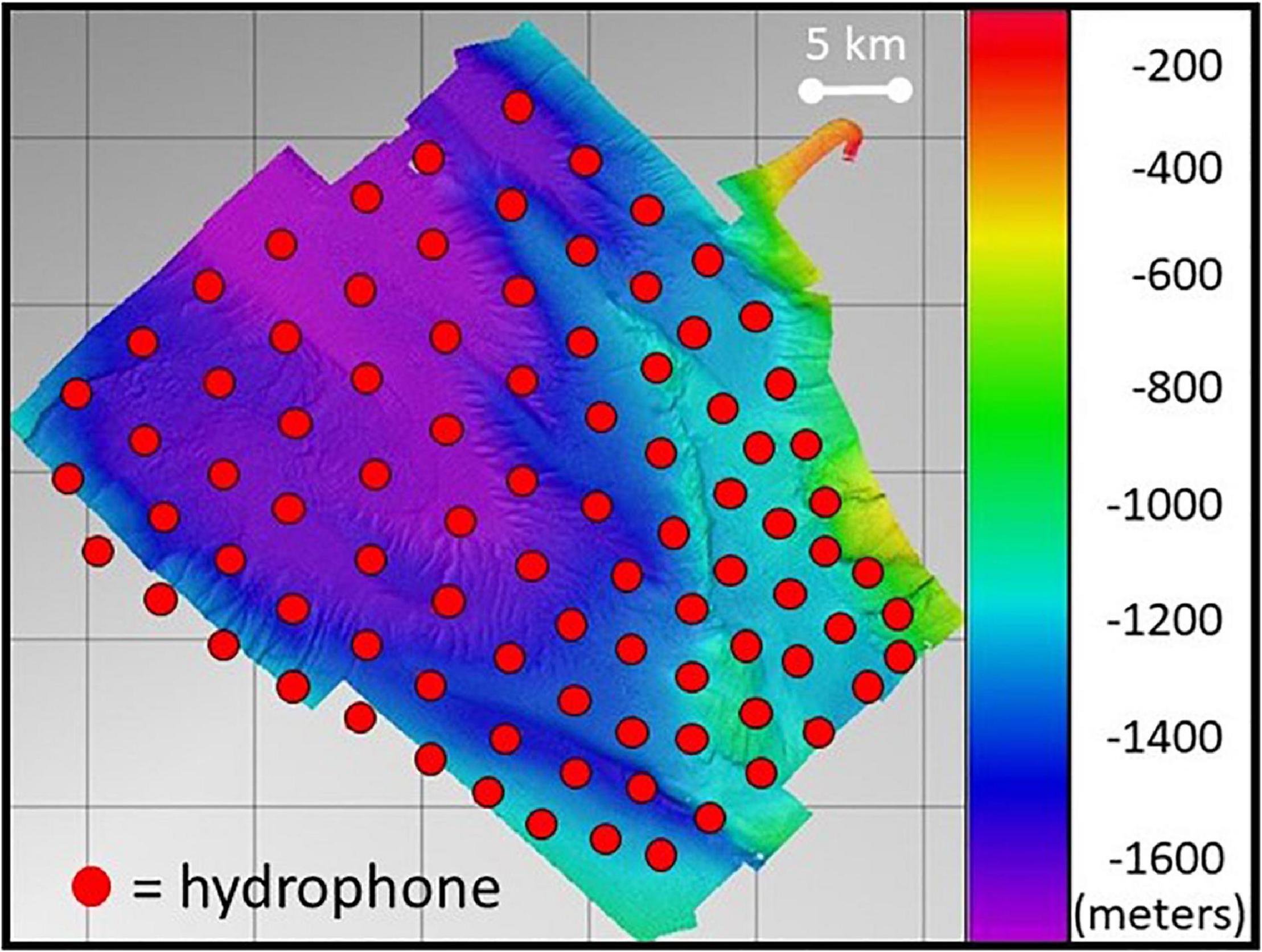
Figure 1. Bathymetry of the SOAR with overlaid 89 hydrophone (red circles) sensors in the array. Depth scale is in meters. Reproduced from Kates Varghese et al. (2020) with the permission of the Acoustical Society of America.

As a follow-on to earlier work assessing the effect of MBES activity on the temporal aspects of Cuvier’s beaked whale foraging behavior (Kates Varghese et al., 2020), the same detection and data processing schemes used in that study were used here. Echolocation clicks from several marine mammal species at the SOAR were detected using a class-specific support vector machine. Those that were classified as Cuvier’s beaked whale foraging clicks were formed into click trains on a per hydrophone basis. Then a MATLAB-based autogrouper program used a set of rules based on the time and location of the click trains to form the GVPs (DiMarzio et al., 2018; Moretti, 2019). A GVP may be detected on multiple hydrophones, but the hydrophone that records the highest click density is defined as the center hydrophone of the event. The center hydrophone was used as the location of a GVP in this study. The maximum detection range of Blainville’s beaked whale clicks was measured at 6.5 km at a U.S. Navy range in the Bahamas by cross-correlating the pattern of clicks identified on a DTAG, produced by the tagged animal, against the click patterns on surrounding bottom-mounted range hydrophones (Ward et al., 2008). These animals have a similar click source level and dive behavior to Cuvier’s beaked whales (Johnson et al., 2004; Tyack et al., 2006). Previous studies at the SOAR have used an estimated horizontal detection distance of 6.3 km in defining a spatial range for Cuvier’s beaked whale clicks detected from a single group (Kates Varghese et al., 2020). This detection range was assumed to be true for this study as well. The number of GVPs, per hydrophone, was used as a proxy to assess spatial foraging effort. For complete details on the detection and processing of GVPs see DiMarzio et al. (2018) and for its application to this work see the Materials and Methods section of Kates Varghese et al. (2020).

The method and data of this research study provide the opportunity to assess the change in overall spatial foraging behavior amongst Cuvier’s beaked whales on the SOAR, i.e., the “foraging effort.” This broad-stroke term is used because it emphasizes that this approach is agnostic to group size and composition, as both attributes can be ephemeral, in addition to other unknown factors such as foraging rates. Past studies of Cuvier’s beaked whales have shown that this species is known to forage in small groups that can vary in composition (Moulins et al., 2007) and change in size (McSweeney et al., 2007). Animals may leave one foraging group and begin foraging with another. A group of animals may leave an area, while another group arrives, and numerous groups could be foraging simultaneously in a particular location (Falcone et al., 2009). Frequently at SOAR it appears that multiple small groups are foraging in the same general area, ensonifying some common hydrophone. Therefore it is important to note that a GVP represents a single detected period of a group of beaked whales foraging, but a GVP is not tied to a specific group of animals. The formation of GVPs is an automated process based on a fixed set of rules, but the group of individuals it represents may differ. Thus this is not an assessment of specific individuals or the behavior of a specific group, rather overall group-level foraging effort.

Two MBES surveys were conducted, one in January 2017 (Mayer, 2017; Smith, 2019) and the other in January 2019 (Mayer, 2019), as part of a MBES characterization project for the Kongsberg EM 122, a deep water MBES. Both surveys utilized the UNOLS research vessel Sally Ride and its hull-mounted EM 122 (12 kHz center frequency) operating with typical parameters used for mapping a deep-water environment such as the SOAR (Table 1). The survey in 2017 followed a characteristic mowing-the-lawn pattern across the entire SOAR (Figure 2 left), whereas the efforts of the 2019 characterization survey required a tighter mowing-the-lawn pattern confined to the canyon in the southeastern corner of the SOAR in addition to a few cross-range lines (Figure 2 right). These surveys served as an opportunity to assess the effect of MBES on the spatial foraging effort of Cuvier’s beaked whales. Because the exact movement of a vessel and hull-mounted MBES will vary from survey to survey based on the needs of the operation, the assessment of the two surveys provided a chance to observe potential variability in beaked whale spatial foraging effort during two separate MBES surveys.

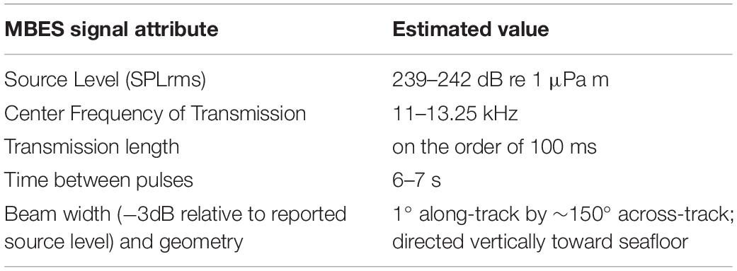
Table 1. MBES signal attributes and the estimated value for the 2017 and 2019 MBES surveys.

Figure 2. Track lines from the 2017 (left) and 2019 (right) MBES surveys.¹ (Reproduced from Kates Varghese et al. (2020) with the permission of the Acoustical Society of America).

In order to assess the effect of MBES activity on the spatial foraging effort of Cuvier’s beaked whales, the number of GVPs were summed by hydrophone over each analysis period: Before, During, and After for each of the two MBES surveys. The same analysis periods assessed in the temporal analysis (Kates Varghese et al., 2020) were used here for consistency (Tables 2, 3 for the 2017 and 2019 surveys, respectively). In the 2017 survey, each analysis period was 47 h long, whereas in 2019, each analysis period was 52 h long. These analysis periods were based on and equivalent to the length of time that the MBES was operating in each year.

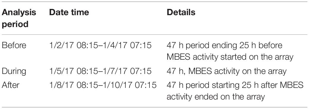
Table 2. Analysis period times and details of the 2017 data set.

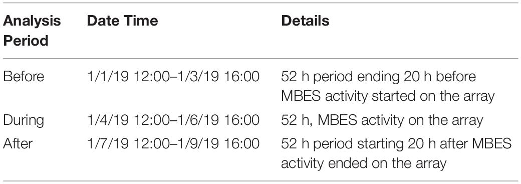
Table 3. Analysis period times and details of the 2019 data set.

Though it was not explicitly addressed in this study, previous research has shown that environmental and oceanographic conditions can affect prey availability on various spatiotemporal scales, impacting marine predator-prey relationships (Sims et al., 2006; Thayer and Sydeman, 2007; Embling et al., 2012; Santora et al., 2014; Cox et al., 2018). Based on this knowledge, it was expected that environmental conditions and prey distributions that could drive the beaked whales’ spatial use of the SOAR would vary on a timescale of less than two years (the time between the two surveys). Thus each survey year was assessed individually.

The GLC approach (Kates Varghese et al., in review), a spatial assessment for analyzing marine mammal behavior on large hydrophone arrays, was used here. This method included two statistical spatial analyses: a global and local approach, as well as comparison analysis of variance tests and visualization tools for interpreting the statistical results. The global analysis used the Moran’s I statistic (Moran, 1948) to provide a coarse assessment of the type of spatial distribution, i.e., clustered, random, or dispersed, of the foraging events over the SOAR as a whole. The local approach used the Getis-Ord Gi^∗ statistic (Getis and Ord, 1992), a local indicator of spatial association (Anselin, 1995), which identifies where relative hot and cold spots of foraging activity occurred on a per hydrophone basis. The comparison analysis used the Kruskal-Wallis test (Kruskal and Wallis, 1952) to identify order-of-magnitude differences in the number of GVPs per hydrophone among analysis periods.

Global Analysis

In order to assess the spatial distribution of the foraging events over the entire SOAR, the global statistic, Moran’s I, was used. Moran’s I measures the overall spatial autocorrelation of a data set, producing a value between (−1, 1). A value of negative one corresponds to perfect dispersion (Figure 3 left), a value of positive one corresponds to perfect clustering of like values (Figure 3 right), and zero represents no autocorrelation, or a perfectly random distribution (Figure 3 middle).

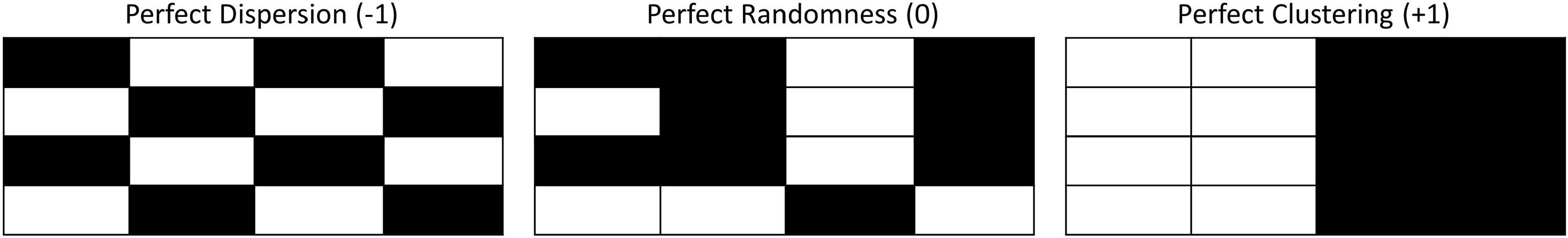
Figure 3. From Kates Varghese et al. (in review). Spatial configurations that would result in ideal Moran’s I values: left – perfect dispersion, Moran’s I value = −1; middle – perfect randomness, Moran’s I value = 0; right – perfect clustering, Moran’s I value = +1.

Moran’s I is given by the formula:

where $W={\sum }_{i=1}^n{\sum }_{j=1}^n{w}_{i,j}$ with w_i,j being the weighting between the i^th and j^th hydrophone and w represents the neighbor weighting matrix of i rows and j columns. x_i refers to the i^th hydrophone value, in this case the number of GVP of the i^th hydrophone and $\overline{x}$ is the mean number of GVPs over all of the hydrophones. A queen’s contiguity neighbor weighting rule was used here as was recommended for similar data in Kates Varghese et al. (in review). The queen criterion defines neighbors as spatial units that share a boundary with the hydrophone of interest (i.e., all hydrophones immediately horizontal, vertical, or diagonal). Thus, the maximum number of neighbors an interior hydrophone could have is eight, whereas edge and corner hydrophones will have fewer.

The Moran’s I statistic for each analysis period was converted to a z-score. To aid in the interpretation of the global results, p-values were computed for each z-score. The smaller the p-value, the greater the discrepancy between the observed data and the null hypothesis being tested (Tanha et al., 2017). The null hypothesis for the Moran’s I analysis was that the spatial distribution of GVPs under consideration, for any of the analysis periods, was no different from random (I = 0). Alternatively, it was hypothesized that the spatial distribution was clustered (I = +1) during each analysis period, Before, During, and After, since beaked whales are known to primarily forage in the deepest part of the SOAR (Falcone et al., 2009; Schorr et al., 2014; DiMarzio et al., 2019; Southall et al., 2019). The Moran’s I statistic, along with the p-value, was used to make a statement about whether the GVPs were clustered or not.

Local Analysis

If global spatial correlation – clustering or dispersion – was detected, the Getis-Ord Gi^∗ (Gi^∗) local statistic was also computed. The Gi^∗ statistic was found for each hydrophone using the formula:

$G_i^{*}=\frac{{\sum }_{j=1}^n{w}_{i,j}{x}_j-\overline{X}{\sum }_{j=1}^n{w}_{i,j}}{S\sqrt{\frac{n{\sum }_{j=1}^n{w}_{i,j}^2-{({\sum }_{j=1}^n{w}_{i,j})}^2}{(n-1)}}}$, where $S=\sqrt{\frac{{\sum }_{j=1}^n{x}_j^2}{n}-{(\overline{X})}^2}$ and $\overline{X}=\frac{{\sum }_{j=1}^n{x}_j}{n}$ and the remaining variables were the same as described for the Moran’s I statistic. This statistic was used to understand where, i.e., on which specific hydrophones, the spatial correlation (relative hot or cold spots) occurred within the SOAR. For example, to be a relative hot spot, a hydrophone must be surrounded by other hydrophones that also exhibit a high number of GVPs and vice-versa for a relative cold spot. What constitutes a high or low number of GVPs will change depending on the specific set of data, their distribution and variance, which are all considered in the Gi^∗ calculation.

P-values associated with each Gi^∗ statistic, which is itself a z-score, were computed to help understand how the observed Gi^∗ results differed from the null hypothesis. The null hypothesis was that GVPs were randomly distributed and thus that there were no relative hot or cold spots of foraging activity. A small p-value indicated a greater discrepancy from this null hypothesis suggesting a spatial anomaly – i.e., an area of congregation or absence. Since there are 89 hydrophones on the SOAR, alternative hypotheses were not made about individual hydrophones. However, it was hypothesized that the northwest part of the SOAR, which has the deepest depths, and where the animals are historically known to forage (Falcone et al., 2009; Schorr et al., 2014; DiMarzio et al., 2019; Southall et al., 2019), would be an area of high foraging activity (i.e., hot spots), while the shallow area in the southeast along San Clemente Island would have low foraging activity (i.e., cold spots). It was hypothesized that the relative hot and cold spots, with respect to foraging, would remain in these respective areas throughout the three analysis periods, which would indicate the spatial distribution of GVPs did not change during MBES activity.

Comparison Analysis

Although the spatial statistics provided insight into spatial changes on the SOAR, they did not provide information about differences in scale, i.e., the average number of GVPs per hydrophone occurring on the SOAR in the various analysis periods. In addition to, or in the absence of a spatial change, understanding potential order-of-magnitude differences in the number of GVPs detected provided further information about the extent of change. Following the GLC approach from Kates Varghese et al. (in review) for similar data, the Kruskal-Wallis test was used to compare the magnitude of observations among different analysis periods. For both years of study, the null hypothesis was that there was no difference in the number of GVPs per hydrophone on the SOAR among the analysis periods. Difference plots of the hydrophone array were also generated to show spatially what the relative change (e.g., increase, decrease, or no change) was in the number of GVPs between consecutive analysis periods.

The GLC approach is further developed and described in more detail in Kates Varghese et al. (in review).

Results

2017

Of the 47 h analyzed for each of the three analysis periods in 2017, there were 127 GVPs detected across the 89 hydrophones Before, 135 During, and 148 After. The results of the global analysis are provided in Table 4. For all analysis periods of 2017, the Moran’s I value suggested strong spatial clustering of GVPs on the SOAR.

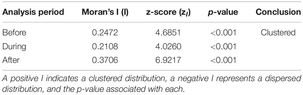
Table 4. Global analysis results by analysis period for 2017, including Moran’s I value (I), the z-score (z_I), and the associated p-value.

The total number of GVPs detected and the respective Gi^∗ z-score for each hydrophone was calculated and is shown in the map presented in the first and second columns, respectively, of Figure 4 for each analysis period of 2017. To aid in the designation and interpretation of hot and cold spots in the Gi^∗ results, p-values equal to or less than 0.1, or equal to and more than 0.9 were mapped along-side the Gi^∗ results (Figure 4, column 3). Hydrophones with p-values of 0.1 or less provided the strongest evidence of hot spots on the Gi^∗ plot, while a p-value of 0.9 or more provided the strongest evidence of a cold spot on the Gi^∗ plot. Exact Gi^∗ and p-values for all hydrophones are provided in the data section of this publication. Ultimately, a critical alpha level of 0.05 was used to guide the final interpretation of the Gi^∗ results. Because of the two-tailed nature of this analysis (hot and cold spots), the authors focused on areas with p-values less than or equal to 0.025 (hot) or greater than or equal to 0.975 (cold) in the descriptive interpretation of the Gi^∗ results that follows.

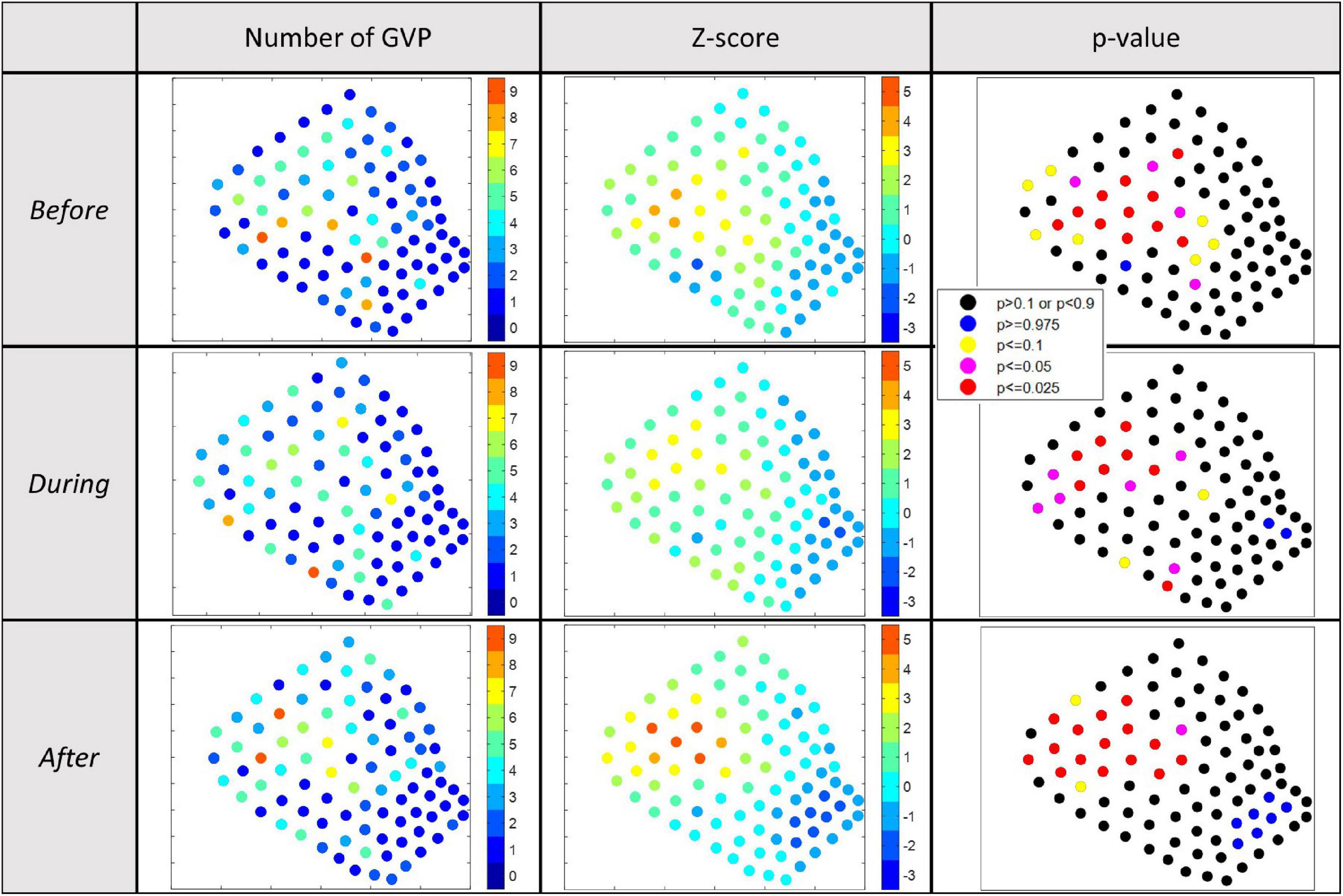
Figure 4. Results of the 2017 Gi* analysis for local hot/cold spots. Column 1: visual depiction of the number of GVPs by hydrophone; column 2: visual depiction of the Gi* z-values by hydrophone; column 3: visual depiction of the p-values associated with the Gi* results by hydrophone. p < 0.025 were considered relative hot spots, whereas p > 0.975 were considered relative cold spots. Each row represents a different analysis period: top-Before; middle-During; bottom-After.

In each analysis period, there was a clustering (i.e., a group of several adjacent hydrophones) of hot spots in the northwest corner of the SOAR (Figure 4, column 3), overlapping the deeper waters of the SOAR (Figure 1). This result matched expectations since this area has historically been noted as favorable foraging grounds for these animals due to the deep-water conditions (Falcone et al., 2009; Schorr et al., 2014), providing ideal habitat for the squid that Cuvier’s beaked whales prey upon (Santos et al., 2001). The exact cluster of hot spot hydrophones shifted slightly between analysis periods. However, based on the recommendation of Kates Varghese et al. (in review) in the development of the GLC approach, the general area of hot/cold spot clusters should be compared rather than employing a precise comparison of individual hydrophones. Since many of the hydrophones in the hot spot cluster were the same across analysis periods and remained in the same general area in the deepest part of the SOAR, this result suggested no obvious change occurred in spatial foraging effort in the 2017 study.

With respect to where there were very few GVPs, there was one cold spot hydrophone in the central-western part of the SOAR in the Before period and a small cluster of hydrophones signifying cold spots in the southeast corner of the SOAR During and After. Overall the southeastern corner – the relatively shallow and historically least-used area (Falcone et al., 2009; Schorr et al., 2014) – was not a high-use area for foraging beaked whales (Figure 4, column 1). Thus, the Gi^∗ analysis further suggested no obvious spatial change occurred in beaked whale foraging effort among analysis periods in 2017 at a local level. This finding was supported by the difference plots for which the spatial distribution of hydrophones that exhibited no change, increase, or decrease in the number of GVPs appeared random (Figure 5).

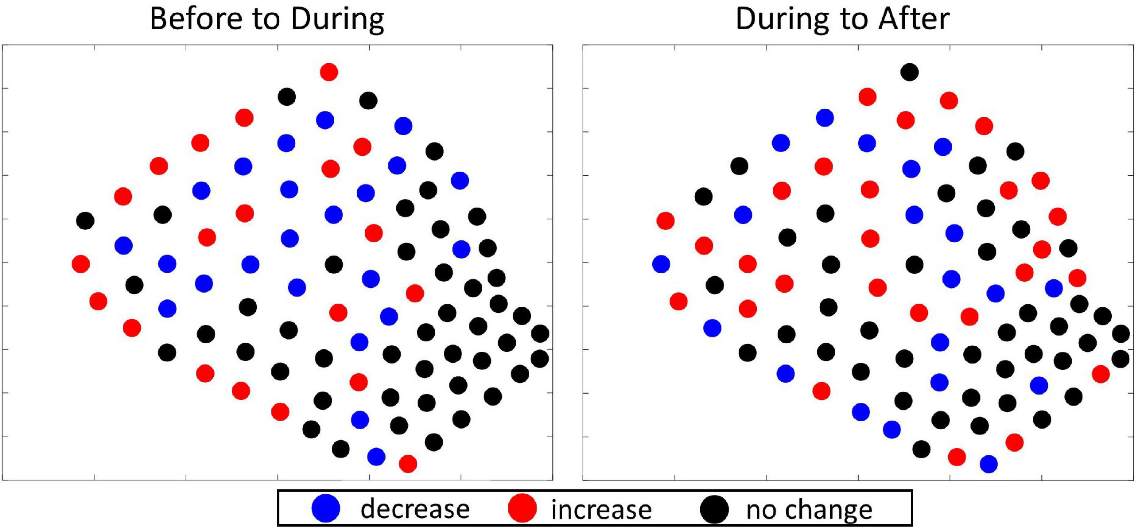
Figure 5. Difference plots showing the direction of change in the number of GVPs per hydrophone from one period to the next of the 2017 survey. Left: difference plot showing change from Before to During; Right: difference plot showing change from During to After.

Not only was there no overall change in the spatial location of relative hot/cold spots among analysis periods, but the Kruskal-Wallis comparison test revealed that the total number of GVPs per hydrophone among the three analysis periods were similar [H (2) = 1.24, p = 0.5369].

Overall the GLC spatial analysis of the 2017 study showed a consistent pattern, both globally and locally, in spatial clustering of GVPs and a similar number of GVPs for non-MBES and MBES analysis periods.

2019

Fifty-two hours of hydrophone data were analyzed for each of the three analysis periods in 2019. There were 60 GVPs detected Before, 93 During, and 77 After. The global analysis results are provided in Table 5. For each of the three analysis periods the Moran’s I value strongly suggested GVPs were spatially clustered on the SOAR.

Table 5. Global analysis results by analysis period for 2019, including Moran’s I value (I), the z-score (z_I), and the associated p-value.

The total number of GVPs detected, the Gi^∗ z-score, and associated p-values were calculated and are shown by hydrophone in Figure 6, columns 1–3, respectively. Exact Gi^∗ and p-values for all hydrophones are provided in the data section of this publication. A similar interpretation of Figure 6 was conducted as described for the interpretation of the 2017 local results. There were no obvious cold spots identified in the 2019 analysis periods, suggesting widespread use of the SOAR by foraging beaked whales in 2019 (Figure 6). There were distinct hot spot clusters identified in each analysis period. In the Before period the hot spot cluster was in the southwestern corner of the SOAR, During MBES activity the hot spot cluster was in the center, and After MBES activity there were several hot spot hydrophones in the center and a cluster of hot spot hydrophones in the southwestern corner of the SOAR (Figure 6). These results suggested that local spatial foraging effort did change during the 2019 study, a finding that was supported by a distinguishable spatial pattern visible in the 2019 difference plots (Figure 7). That is, there was a cluster of hydrophones in the center of the SOAR that all recorded an increase in GVPs from Before to During (Figure 7 left), while from During to After (Figure 7 right) there was a cluster of hydrophones in the center that all decreased in the number of GVPs.

Figure 6. Results of the 2019 Gi* analysis for local hot/cold spots. Column 1: visual depiction of the number of GVPs by hydrophone; column 2: visual depiction of the Gi* z-values by hydrophone; column 3: visual depiction of the p-values associated with the Gi* results by hydrophone. p < 0.025 were considered relative hot spots, whereas p > 0.975 were considered relative cold spots. Each row represents a different analysis period: top-Before; middle-During; bottom-After.

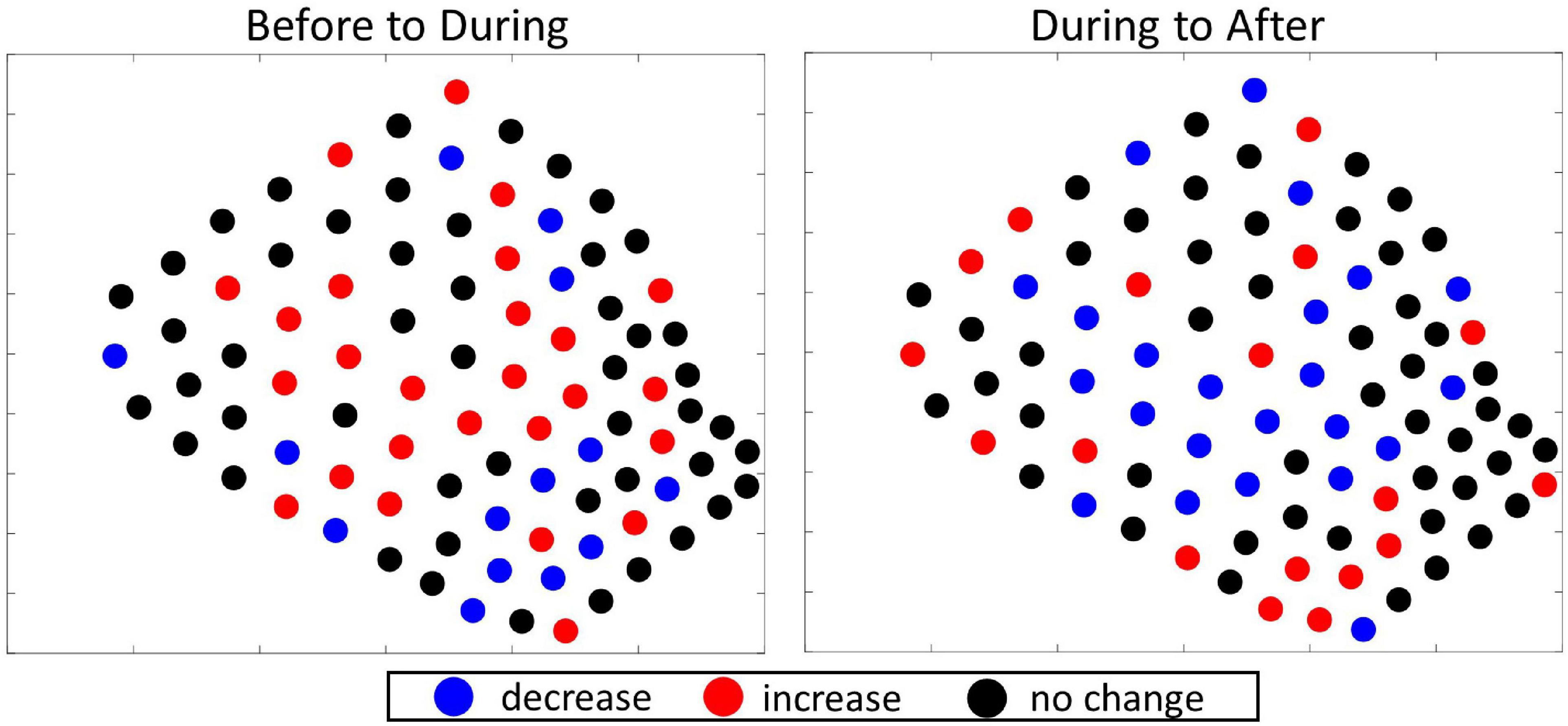
Figure 7. Difference plots showing the direction of change in the number of GVPs per hydrophone from one period to the next of the 2019 survey. Left: difference plot showing change from Before to During; Right: difference plot showing change from During to After.

The Kruskal-Wallis comparison test showed that the number of GVPs per hydrophone were similar between the three analysis periods [H (2) = 3.95, p = 0.1387].

Overall the GLC spatial analysis of the 2019 study showed foraging effort was consistently clustered, and the overall magnitude of foraging effort was similar throughout the 2019 analysis periods. But, the location of the foraging hot spot cluster changed through time.

Discussion

The global analysis revealed that GVPs on the SOAR were notably clustered spatially in all analysis periods in both 2017 and 2019. In addition, the comparison tests for both years revealed that the overall number of GVPs detected per hydrophone was equivalent among analysis periods within each year. These results suggest that no obvious range-wide change in foraging effort occurred during MBES activity. The local results for the two surveys were not the same. In 2017, foraging hot and cold spots were, respectively, identified in the same general area of the SOAR during all three analysis periods. In 2019, foraging hot spots were identified in each analysis period, but the location shifted through time. Like the temporal analysis of foraging behavior during the two MBES surveys (Kates Varghese et al., 2020), the difference in local spatial results between the two years brings in to question whether the MBES activity (i.e., different spatial usage of the SOAR) could have contributed to the differences identified, or if the differences were related to variability in some other factor, such as prey distribution during the two years of study.

The results of the 2017 local analysis identified relative hot and cold spots in the same general area of the SOAR, but during each period on a slightly different set of hydrophones in the array. There are likely multiple interacting reasons for the slight difference in cluster locations. Firstly, even if the animals tend to forage in the same area throughout time, it is within reason to expect some amount of variation due to the natural variability in behavior (e.g., the animals are mobile, peaks and lulls in foraging are observed even in the absence of anthropogenic activity) (Schorr et al., 2014; Falcone et al., 2017), and because a cluster likely represents numerous groups foraging, each with their own movements over the wider area. Additionally, there may have been small changes in the distribution of prey, due to varying environmental conditions, which could have affected exact foraging locations. Lastly, the Gi^∗ statistic, the statistic used in the local analysis, is a function not only of the number of GVPs at a specific hydrophone, but of its neighboring hydrophones as well. This can lead to a slightly different spatial z-score pattern, despite a generally very similar spatial data set. For this reason Kates Varghese et al. (in review) recommended that it is most appropriate to interpret change in spatial behavior using the GLC approach more holistically than on a single hydrophone basis to account for some of the sensitivity in the Gi^∗ statistic. Most of the GVPs occurred in the northwest and north-central parts of the array and were lacking in the southeast. Since many of the hot spot hydrophones overlapped from one period to the next, there was no indication from this analysis that the area used for foraging had changed in an obvious way that would suggest the 2017 MBES survey had an effect.

The interpretation of the local analysis result for 2019 was less clear. Before the MBES survey, a distinct cluster of foraging hot spots was identified in the southwestern corner of the SOAR, During the survey a distinct cluster of foraging hot spots was identified in the center, and After there was a distinct hot spot cluster in the southwestern corner and potentially another hot spot cluster in the center of the SOAR. In general, the hot spot clusters had minimal overlap across abutting analysis periods, suggesting there was a change in foraging effort at the local level. But the pattern of two potential hot spot clusters identified in the After period was perplexing. Specifically, the potential cluster in the center of the array After was not as obvious as other clusters, raising the question of whether the center of the SOAR was in fact a highly used area by the animals during this period. Whether it was or not would provide information that could help in ruling out certain potential drivers of the 2019 result.

Referring to the spatial distribution of the 2019 raw data, z-scores, and difference plots provided further insight in interpreting the local result. The spatial distribution of high versus low GVP values After appeared random in the center area, suggesting it was only a few hydrophones where many GVPs occurred and not the entire area. In addition, the z-scores of hydrophones in the center in the After period were lower in comparison to all of the other hot spot clusters from any of the 2019 analysis periods – i.e., the center area hydrophones of the After period had a z-score value of mostly twos, while all other hot spots had z-scores of mostly threes or fours. This suggests that although there were a high number of GVPs in the center, it was not the most highly used area relative to the rest of the SOAR. In fact, the southwestern corner had higher z-score values during the same period. In examining the difference plots, none of the center hot spot hydrophones increased in the number of GVPs from During to After, and most of the GVP values on surrounding hydrophones in the center either decreased or stayed the same, whereas those in the southwestern corner had an increase in GVPs detected. Again, this result suggests that the center was not as active as the southwestern corner of the SOAR After the survey. Together, these results best support the interpretation that the center area was no longer as favored by the animals for foraging as it was in the During period.

If the spatial change was due to the MBES survey, one would expect a more discrete difference between each set of analysis periods, and thus a clear change back to the southwestern corner After. For example, in the McCarthy et al. (2011) in which the analysis periods abutted temporally, there was a distinct spatial change between the Before, During, and After analysis periods. In a finer temporal analysis of the spatial data, the researchers found that the animals returned to their normal spatial use of the range after 35 h. In the study herein, there were 20 h between each set of analysis periods in 2019, and each analysis period lasted 52 h. If the MBES was the cause of spatial change, assuming a similar response time as in the MFAS study, the temporal spacing in this study (i.e., time between analysis periods plus the duration of an analysis period) should have been more than adequate to capture distinct differences in foraging effort location. If the spatial change was due to a factor that was primarily a function of time rather than related to the MBES survey, one might expect a more gradual spatial change across all three analysis periods. But what occurred was a distinct change in foraging effort (i.e., relative hot spots) location from Before to During and a spatial pattern suggestive of a gradual change from During to After, a response somewhere in between the two scenarios that were expected. Thus, it is not readily obvious what the cause of the shift was.

There is no standard definition of what constitutes a meaningful shift in habitat use, especially in the context of response to anthropogenic activity or some other external factor. A meaningful shift in habitat use depends on a number of factors including the behavioral or ecological context for which the shift occurs, the species, suitable habitat connectivity, among many other factors. In the case where a group of animals is negatively affected by a disturbance, there may exist circumstances where either no suitable alternative habitat exists for the animals to move to, or the animals endure the disturbing activity despite potential and realized biological consequences (Claridge, 2013; Moretti, 2019). In addition the degree to which an easily observable response, such as behavior change, correlates with a meaningful effect, such as biological or physiological change, is not often known (Beale, 2007). Our ability to understand the degree to which a measured behavioral response is indicative of something meaningful requires comprehensive integration of the information available regarding the factors under which the behavioral change took place, as well as consideration of other known analogs. With this in mind, potential explanations for the observed shift in spatial use of the SOAR by beaked whales were explored.

Since the 12 kHz MBES sound is within the hearing range of beaked whales (Cook et al., 2006; Pacini et al., 2011), one explanation for a shift in foraging location is that the whales were disturbed by the anthropogenic activity on the SOAR, e.g., vessel presence, vessel noise, or MBES activity. In the case of a disturbance, movement would be expected away from the disturbing activity. This was the case with beaked whales in response to other sources within their hearing range, such as MFAS (McCarthy et al., 2011; Manzano-Roth et al., 2016) and acoustic pingers (Carretta et al., 2008). In both the McCarthy et al. (2011) and Manzano-Roth et al. (2016) studies, where a clear negative response to MFAS activity was concluded, the number of GVPs of Blainville’s beaked whales was reduced and the majority of foraging shifted to the edge or off the range during MFAS activity. In the case of the acoustic pingers (10–12 kHz), bycatch of several beaked whale species was reduced to zero after the implementation of the pingers on gillnets in the California drift gill net fishery (Carretta et al., 2008). Neither of these were similar to the result seen here.

Alternatively, a shift in foraging effort location could also be due to attraction of the whales to the anthropogenic activity. During the first 24 h of the 2019 MBES survey (i.e., roughly half of the During period) the MBES survey was confined to the southeast corner of the SOAR (see Figure 2 and the supplementary results of Kates Varghese et al. (2020) for a detailed description of the MBES surveys). Therefore, one might expect if the whales were attracted to the MBES sound that they might move to the southeast corner. Yet, this was not where the foraging hot spots were found. The remainder of the During period involved lines that ran across the center of the SOAR in a “mowing-the-lawn” pattern. Given that the MFAS study results (McCarthy et al., 2011; Manzano-Roth et al., 2016) are viewed as an avoidance response, where many of the animals moved to the edge or off the range, one might view a shift in foraging effort to the center of the SOAR during anthropogenic activity as movement toward, or an attraction to, the activity. In this case it is worth considering the sound propagation of the deep-water MBES on the SOAR. MBES transmit sound toward the seafloor in a beam that is narrow along-track (1°) and broad (∼150°) across-track (Lurton, 2016; Kates Varghese et al., 2019a). As a result, most of the energy is directed toward the seafloor directly below the vessel as lines are run over the survey area, reducing the acoustic footprint relative to an omni-directional or horizontally transmitting source (Lurton and DeRuiter, 2011; Lurton, 2016). A preliminary examination of some of the acoustic data from the hydrophone array from the 2017 survey revealed that the signal from the MBES was only detectable above the noise floor when the vessel was within 10–15 kilometers, or roughly 2–3 hydrophones, from a given hydrophone (Mayer, 2019; Kates Varghese et al., 2019b). The acoustic data from the array was not available for the 2019 survey as of the writing of this paper, but it is reasonable to expect that the sound propagation during the 2019 survey was similar to the 2017 survey since the survey utilized the same vessel, MBES, and was conducted in a similar sea state (Mayer, 2019). Since the MBES was not stationary during the survey, a distance of 10–15 km or less between the vessel and a group of foraging whales was likely only met a small portion of the time. Based on this, one might expect that if the whales heard and were attracted to the MBES that the spatial pattern of their foraging would more closely follow the track lines. This would likely lead to the detection of a more random spatial pattern in the local results than the clustering in the center seen here. Thus it does not seem probable that an attraction to the sound was the cause of the spatial change. However, a full analysis of the soundscape with respect to the distribution of GVPs would be needed to rule this out completely.

Another explanation for a shift in foraging location is due to a change in prey distribution, since foraging behavior in beaked whales is heavily driven by prey dynamics (Benoit-Bird et al., 2016, 2020; Southall et al., 2019). The anthropogenic activity could have disturbed or attracted the prey, leading to a change in their distribution (Fewtrell and McCauley, 2012), followed by a change in where the whales foraged. Beaked whales primarily forage on deep-water squid (Santos et al., 2001) and some fish, both of which are thought to primarily detect low-frequency (<1 kHz) acoustic signals (in addition to particle motion) (Mooney et al., 2010; Popper and Hawkins, 2018). Thus it seems unlikely that such prey species would respond to the 12 kHz MBES signal. It is possible that the prey could detect and respond to vessel noise, which is lower in frequency (<1 kHz). Prey distribution and patchiness can also vary naturally due to normal prey movement over time and/or in response to spatially variable and temporally changing environmental conditions (Benoit-Bird et al., 2013, 2020). In fact, recent work has shown that within the SOAR, prey fields are heterogeneous over small distances (Southall et al., 2019). It is also possible that a specific prey patch was depleted by foraging whales, resulting in their movement to another prey patch elsewhere on the SOAR. Backscatter data from sonar systems can be used to identify squid and other prey items in the water column (Moline and Benoit-Bird, 2016; Southall et al., 2019), and be used to explore these prey distribution hypotheses. However, the signal needed to achieve an adequate estimate of biological organisms at the depths relevant to beaked whale foraging is not feasible from a traditional hull-mounted MBES (Moline and Benoit-Bird, 2016), like the one used in this study. Given the results of this study and the hypotheses explored here, the most probable explanation of the 2019 result is linked to the strong relationship between foraging behavior and prey field dynamics. Without complementary prey field information this cannot be concluded with certainty.

Although there was a change in the spatial use of the array in 2019 and the cause remains unclear there are a few key observations to take away from the 2019 survey. First, the most highly utilized location by the foraging animals (i.e., relative foraging hot spot) remained in the deeper area of the SOAR during all analysis periods. Despite the deeper waters being identified in past studies as the area where these animals forage (Falcone et al., 2009; Schorr et al., 2014), there may still be negative implications for a shift within this area (i.e., from the southwest to the center). Southall et al. (2019) found that even within small areas of the SOAR (the west versus the east for example) prey density can be quite different, which can have huge repercussions on the energetic costliness of an induced spatial change from favorable to unfavorable foraging grounds (Moretti, 2019). However, the number of GVPs detected during the MBES survey period was no different than the non-survey periods. Assuming there was no change in the number of animals foraging, this would suggest that there was not an overall change in foraging effort. Furthermore, the fine-scale temporal analysis of the 2019 survey showed no difference in two other GVP characteristics (i.e., number of clicks per GVP, and click rate per GVP) during the MBES survey versus non-MBES periods (Kates Varghese et al., 2020). These results further suggest that there was little change in how the animals were foraging. If there were obvious differences in the number of GVPs and intrinsic characteristics (i.e., number of clicks, click rate) of the GVP, this might suggest there was a change in the quality of the prey field with respect to foraging. In the absence of prey distribution data for this study, these results suggest that the spatial change identified may not be associated with a high energetic cost to the animals. Future studies assessing MBES impact should integrate prey field assessments to verify this. This is extremely important in being able to assess the biological and ecological relevance of a change in behavior.

The spatial change in the 2019 study and absence of change in 2017 raises the question, why was there a difference between the two years? Both surveys were conducted in January, removing potential seasonal differences in beaked whale ecology that might affect behavior. The surveys were also conducted using the same vessel and 12 kHz MBES, and occurred for similar lengths of time (47 h in 2017 versus 52 h in 2019). The only known difference between the two surveys were the line plans. The 2017 survey was conducted in a mowing-the-lawn pattern across the full length of the array, whereas the 2019 survey used a tighter mowing-the-lawn pattern confined to the southeast corner of the SOAR before conducting a few full-length passes across the middle of the SOAR. As discussed previously, the spatial change found in the 2019 study does not appear to be driven by MBES activity, so it would seem unlikely that the different line plans were the reason for the inter-annual differences. However, without further evaluation of some or all of the hypotheses posed here, this hypothesis should not be disregarded. It should be noted though that while the “mowing the lawn” survey conducted in 2017 is representative of a typical MBES mapping survey, the localized MBES survey in 2019 was conducted particularly to assess the beam pattern of the MBES system and is not at all representative of the use of MBES in deep-water ocean mapping work.

It is worth drawing attention to the spatial distribution of GVPs in the non-MBES periods before the surveys were conducted. These were also dissimilar between the two years. In 2017, there was relatively minimal GVP activity in the southeast portion of the SOAR, whereas in 2019 there was more widespread use of the entire SOAR. These patterns were seen throughout each respective year, suggesting that there was simply variation in the use of the SOAR by the animals from one year to the next. If the spatial distribution Before MBES activity was different between the two years, one cannot therefore assume that the difference between the two years was related to the anthropogenic activity or differences related to the operation of the MBES. Again, since prey distribution heavily dictates where these animals forage, there were very likely differences between prey patches in the two years that led to differences in use of the range both during and outside of periods of anthropogenic activity. Though, this may not be the only possible explanation for differences in spatial use of the SOAR between the two years.

Finally, it is important to keep in mind that the spatial statistics used here can only detect patterns at the resolution of the hydrophone array. Any potential changes in the spatial use of the array that happened on a scale finer than the hydrophone spacing of two to six kilometers were not detected. Spatial change in foraging behavior may occur on a different spatial resolution than was measured here and may have a different consequence on foraging animals. Animal tagging studies and those that focus on individual behavior provide a necessary understanding of finer-scale changes in behavior and potential impacts of anthropogenic noises and should be undertaken with respect to MBES impact where possible in the future.

Conclusion

The overall findings of this spatial analysis align with the conclusions of the temporal assessment (Kates Varghese et al., 2020): foraging effort did not change in a stereotyped way that would suggest that the MBES surveys had a clear negative effect. In both years of study, neither the range-wide or order-of-magnitude comparisons revealed any obvious differences in beaked whale foraging during the MBES surveys. In the 2017 MBES survey there was no indication that the overall foraging effort changed spatially on a local level. During the 2019 MBES survey there was a change detected in the local spatial use of the SOAR. The change was a shift in the most foraging activity toward the center of the range, which was unlike the typical avoidance response seen several times in studies assessing beaked whale foraging response to MFAS. It was also a shift that remained in the deep-water area of the SOAR, thought to be favorable foraging grounds for beaked whales. This best supports the prey-dependence hypothesis as the cause of spatial change. However, the cause of this change and its overall impact cannot be stated with certainty. Future studies targeting the hypotheses posed here are needed to understand the 2019 result completely and should integrate animal tagging, prey field, and soundscape assessments to establish a more comprehensive picture.

Data Availability Statement

The datasets presented in this article are not readily available because of security concerns related to the hydrophone locations. The processed data without the hydrophone locations are available with this manuscript. The raw data may be available on a case-by-case basis. Requests to access the datasets should be directed to ND, nancy.dimarzio@navy.mil.

Author Contributions

DM, ND, LM, JM-O, and HK were involved in the coordination of the field component of this study. ND processed the acoustic data and provided the GVP data for this analysis. HK through the guidance of KL performed the reported analyses. JM-O, KL, and LM provided guidance to HK on the interpretation and communication of the findings of this work. All authors discussed the results and contributed to the final manuscript.

Funding

This material was based upon work supported by the National Science Foundation under grant no. 1524585 and NOAA grant no. NA15NOS4000200 provided to the Center for Coastal and Ocean Mapping at the University of New Hampshire.

Conflict of Interest

The authors declare that the research was conducted in the absence of any commercial or financial relationships that could be construed as a potential conflict of interest.

Publisher’s Note

All claims expressed in this article are solely those of the authors and do not necessarily represent those of their affiliated organizations, or those of the publisher, the editors and the reviewers. Any product that may be evaluated in this article, or claim that may be made by its manufacturer, is not guaranteed or endorsed by the publisher.

Acknowledgments

This study was possible thanks to collaborations with the Scripps Institute of Oceanography and the Office of Naval Research for ship time on the R/V Sally Ride and the U.S. Navy for the time on the SOAR range. Thank you to Stephanie Watwood at the Naval Undersea Warfare Center for supporting this project.

Supplementary Material

The Supplementary Material for this article can be found online at: https://www.frontiersin.org/articles/10.3389/fmars.2021.654184/full#supplementary-material

References

Anselin, L. (1995). Local indicators of spatial association – LISA. Geogr. Anal. 27, 93–115. doi: 10.1111/j.1538-4632.1995.tb00338.x
Beale, C. M. (2007). The behavioral ecology of disturbance responses. Int. J. Comp. Psychol. 20, 111–120.
Benoit-Bird, K. J., Battaile, B. C., Heppell, S. A., Hoover, B., Irons, D., Jones, N., et al. (2013). Prey patch patterns predict habitat use by top marine predators with diverse foraging strategies. PLoS One 8:e53348. doi: 10.1371/journal.pone.0053348
Benoit-Bird, K. J., Southall, B. L., and Moline, M. A. (2016). Predator-guided sampling reveals biotic structure in the bathypelagic. Proc. Biol. Sci. 283:20152457. doi: 10.1098/rspb.2015.2457
Benoit-Bird, K. J., Southall, B. L., Moline, M. A., Claridge, D. E., Dunn, C. A., Dolan, K. A., et al. (2020). Critical threshold identified in the functional relationship between beaked whales and their prey. Mar. Eco. Prog. Ser. 654, 1–16. doi: 10.3354/meps13521
Blom, E. L., Kvarnemo, C., Dekhla, I., Schold, S., Andersson, M. H., Svensson, O., et al. (2019). Continuous but not intermittent noise has a negative impact on mating success in a marine fish with paternal care. Nat. Sci. Rep. 9:5494. doi: 10.1038/s41598-019-41786-x
Carretta, J. V., Barlow, J., and Enriquez, L. (2008). Acoustic pingers eliminate beaked whale bycatch in a gill net fishery. Mar. Mamm. Sci. 24, 956–961. doi: 10.111/j.1748-7692.2008.00218.x
Cholewiak, D., DeAngelis, A., Palka, D., Corkeron, P., and Van Parijs, S. (2017). Beaked whales demonstrate a marked acoustic response to the use of shipboard echosounders. R. Soc. Open Sci. 4:170940. doi: 10.1098/rsos.170940
Claridge, D. E. (2013). Population Ecology of Blainville’s Beaked Whales (Mesoplodon Densirostris). Ph.D. Thesis. St Andrews: University of St. Andrews.
Cook, M. L. H., Varela, R. A., Goldstein, J. D., McCulloch, S. D., Bossart, G. D., Finneran, J. J., et al. (2006). Beaked whale auditory evoked potential hearing measurements. J. Comp. Physiol. A 192, 489–495. doi: 10.1007/s00359-005-0086-1
Cox, S. L., Embling, C. B., Hosegood, P. J., Votier, S. C., and Ingram, S. N. (2018). Oceanographic drivers of marine mammal and seabird habitat-use across shelf-seas: a guide to key features and recommendations for future research and conservation management. Estuar. Coast. Shelf Sci. 212, 294–310. doi: 10.1016/j.ecss.2018.06.022
Croll, D. A., Clark, C. W., Calambokidis, J., Ellison, W. T., and Tershy, B. R. (2006). Effect of anthropogenic low-frequency noise on the foraging ecology of Balaenoptera whales. Anim. Conserv. 4, 13–27. doi: 10.1017/S1367943001001020
D’Amico, A., and Pittenger, R. (2009). A brief history of active sonar. Aquat. Mamm. 35, 426–434. doi: 10.1578/AM.35.4.2009.426
DeRuiter, S. L., Southall, B. L., Calambokidis, J., Zimmer, W. M. X., Sadykova, D., Falcone, E. A., et al. (2013). First direct measurements of behavioral responses by Cuvier’s beaked whales to mid-frequency active sonar. Biol. Lett. 9:20130223. doi: 10.1098/rsbl.2013.0223
DiMarzio, N., and Jarvis, S. (2016). Temporal and Spatial Distribution and Habitat Use of Cuvier’s Beaked Whales on the U.S. Navy’s Southern California Antisubmarine Warfare Range (SOAR): Data Preparation. Newport: Naval Undersea Warfare Center.
DiMarzio, N., Jones, B., Moretti, D., Thomas, L., and Oedekoven, C. (2018). Marine Mammal Monitoring on Navy Ranges (M3R) on the Southern California Offshore Range (SOAR) and the Pacific Missile Range Facility (PMRF)− 2017. Newport: Naval Undersea Warfare Center.
DiMarzio, N., Watwood, S., Fetherston, T., and Moretti, D. (2019). Marine Mammal Monitoring on Navy Ranges (M3R) on the Southern California Anti-Submarine Warfare Range (SOAR) and the Pacific Missile Range Facility (PMRF) 2018. Newport: Naval Undersea Warfare Center.
Embling, C. B., Illian, J., Armstrong, E., van der Kooij, J., Sharples, J., Camphuysen, K. C. J., et al. (2012). Investigating fine-scale spatio-temporal predator-prey patterns in dynamic marine ecosystems: a functional data analysis approach. J. Appl. Ecol. 49, 481–492. doi: 10.1111/j.1365-2664.2012.02114.x
Erbe, C., and Farmer, D. M. (2000). Zones of impact around icebreakers affecting beluga whales in the Beaufort Sea. J. Acoustic. Soc. Am. 108, 1332–1340. doi: 10.1121/1.1288938
Evans, D. L., and England, G. R. (2001). Joint Interim Report Bahamas Marine Mammal Stranding Event of 15-16 March 2000, U.S. Washington, DC: Department of Commerce and Secretary of the Navy.
Falcone, E. A., Schorr, G. S., Douglas, A. B., Calambokidis, J., Henderson, E., McKenna, M. F., et al. (2009). Sighting characteristics and photo-identification of Cuvier’s beaked whales (Ziphius cavirostris) near San Clemente Island, California: a key area for beaked whales and the military? Mar. Biol. 156, 2631–2640. doi: 10.1007/s00227-009-1289-8
Falcone, E. A., Schorr, G. S., Watwood, S. L., DeRuiter, S. L., Zerbini, A. N., Andrews, R. D., et al. (2017). Diving behaviour of Cuvier’s beaked whales exposed to two types of military sonar. R. Soc. Open Sci. 4:170629. doi: 10.1098/rsos.170629
Fernandez, A., Sierra, E., Martin, V., Mendez, M., Sacchinnin, S., Bernaldo de Quiros, Y., et al. (2012). Last “atypical” beaked whales mass stranding in the Canary Islands (July, 2004). J. Mar. Sci. Res. Dev. 2:107. doi: 10.4172/2155-9910.1000107
Fewtrell, J. L., and McCauley, R. D. (2012). Impact of air gun noise on the behavior of marine fish and squid. Mar. Pollut. Bull. 64, 984–993. doi: 10.1016/j.marpolbul.2012.02.009
Getis, A., and Ord, J. K. (1992). The analysis of spatial association by use of distance statistics. Geogr. Anal. 24, 189–206. doi: 10.1111/j.1538-4632.1992.tb00261.x
Gomez, C., Lawson, J. W., Wright, A. J., Buren, A. D., Tollit, D., and Lesage, V. (2016). A systematic review on the behavioural responses of wild marine mammals to noise: the disparity between science and policy. Can. J. Zool. 94, 801–819. doi: 10.1139/cjz-2016-0098
Hildebrand, J. (2005). “Impacts of Anthropogenic sound,” in Marine Mammal Research: Conservation Beyond Crisis, eds J. E. Reynolds II, W. F. Perrin, R. R. Reeves, S. Montgomery, and T. J. Ragen (Baltimore, MD: The Johns Hopkins University Press), 101–124.
Isojunno, S., Cure, C., Kvadsheim, P. H., Lam, F. P. A., Tyack, P. L., Wensveen, P. J., et al. (2016). Sperm whales reduce foraging effort during exposure to 1-2 kHz sonar and killer whale sounds. Ecol. Appl. 26, 77–93. doi: 10.1890/15-0040
Jarvis, S. M., Morrisey, R. P., Moretti, D. J., DiMarzio, N. A., and Shaffer, J. A. (2014). Marine mammal monitoring on navy ranges (M3R): a toolset for automated detection, localization, and monitoring of marine mammals in open ocean environments. Mar. Technol. Soc. J. 48, 5–20. doi: 10.4031/mtsj.48.1.1
Johnson, C. E. (2012). “Regulatory assessments of the effects of noise: moving from threshold shift and injury to behavior,” in The Effects of Noise on Aquatic Life, eds A. N. Popper and A. Hawkins (New York, NY: Springer), 563–565. doi: 10.1007/978-1-4419-7311-5_127
Johnson, M., Madsen, P. T., Zimmer, W. M. X., Aguilar de Soto, N., and Tyack, P. L. (2004). Beaked whales echolocate on prey. Proc. Biol. Sci. 271, S383–S386.
Kastelein, R. A., Helder-Hoek, L., Van de Voorde, S., von Benda-Bechmann, S., Lam, F. P. A., Jansen, E., et al. (2017). Temporary hearing threshold shift in a harbor porpoise (Phocoena phocoena) after exposure to multiple airgun sounds. J. Acoust. Soc. Am. 142, 2430–2442. doi: 10.1121/1/5007720
Kates Varghese, H., Miksis-Olds, J., DiMarzio, N., Lowell, K., Linder, E., Mayer, L. A., et al. (2020). The Effect of two 12 kHz Multibeam mapping surveys on the foraging behavior of cuvier’s beaked whales off of Southern California. J. Acoustic. Soc. Am. 147, 3849–3858. doi: 10.1121/10.0001385
Kates Varghese, H., Smith, M. J., Miksis-Olds, J. L., and Mayer, L. (2019a). Regulation consideration of ocean mapping multibeam echo sounders: a square peg in a round hole. J. Ocean Technol. 14, 40–46.
Kates Varghese, H., Smith, M. J., Miksis-Olds, J. L., and Mayer, L. (2019b). The contribution of 12 kHz multibeam sonar to a southern California marine soundscape. J. Acoustic. Soc. Am. 145:1671. doi: 10.1121/1.5101132
Ketten, D. R. (2014). Sonars and strandings: are beaked whales the aquatic acoustic canary? Acoust. Today 10, 45–55.
Kruskal, W. H., and Wallis, W. A. (1952). Use of ranks in one-criterion variance analysis. J. Am. Stat. Assoc. 47, 583–621. doi: 10.1080/01621459.1952.10483441
Lurton, X. (2016). Modelling of the sound field radiated by multibeam echosounders for acoustical impact assessment. Appl. Acoust. 101, 201–221. doi: 10.1016/j.apacoust.2015.07.012
Lurton, X., and DeRuiter, S. (2011). Sound radiation of seafloor-mapping echosounders in the water column, in relation to the risks posed to marine mammals. Int. Hydrogr. Rev. 6, 7–17.
Malme, C. I., Miles, P. R., Clark, C. W., Tyack, P., and Bird, J. E. (1984). Investigations of the Potential Effects of Underwater Noise From Petroleum-Industry Activities on Migrating Gray-Whale Behavior. Phase 2: January 1984 Migration Report Number: PB-86-218377/XAB; BBN-5586. Cambridge, MA: U.S. Department of Energy Office of Scientific and Technical Information.
Manzano-Roth, R., Henderson, E., Martin, S., Martin, C., and Matsuyama, B. (2016). Impacts of U.S. navy training events on Blainville’s beaked whale (Mesoplodon densirostris) foraging dives in Hawaiian waters. Aquat. Mamm. 42, 507–528. doi: 10.1578/am.42.4.2016.507
Marine Mammal Commission (2015). The Marine Mammal Protection Act of 1972 As Amended. Bethesda, MD: NOAA National Marine Fisheries Service.
Mayer, L. (2017). Performance and Progress Report University of New Hampshire/National Oceanic and Atmospheric Administration Joint Hydrographic Center 2017. NOAA Grant No. NA15NOS4000200. Available online at: https://ccom.unh.edu/sites/default/files/progress_reports/2017-jhc-ccom-progress-report-web.pdf (accessed December 23, 2020).
Mayer, L. (2019). University of New Hampshire/National Oceanic and Atmospheric Administration Joint Hydrographic Center 2019 Performance and Progress Report. NOAA Grant No. NA15NOS4000200. Available online at: https://ccom.unh.edu/sites/default/files/progress_reports/2019-jhc-ccom-full-annual-report.pdf (accessed December 23,2020).
McCarthy, E., Moretti, D., Thomas, L., DiMarzio, N., Morrissey, R., Jarvis, S., et al. (2011). Changes in spatial and temporal distribution and vocal behavior of Blainville’s beaked whales (Mesoplodon densirostris) during multiship exercises with mid-frequency sonar. Mar. Mamm. Sci. 27, E206–E226. doi: 10.1111/j.1748-7692.2010.00457.x
McSweeney, D. J., Baird, R. W., and Mahaffy, S. D. (2007). Site fidelity, associations, and movements of Cuvier’s (Ziphius cavirostris) and Blainville’s (Mesoplodon densirostris) beaked whales off the island of Hawai’i. Mar. Mamm. Sci. 23, 666–687. doi: 10.1111/j.1748-7692.2007.00135.x
Miller, P. J. O., Kvadsheim, P. H., Lam, F. P. A., Wensveen, P. J., Antunes, R., Alves, A. C., et al. (2012). The severity of behavioral changes observed during experimental exposures of Killer (Orcinus orca), long-finned pilot (Globicephala melas), and Sperm (Physeter microcephalus) whales to naval sonar. Aquat. Mamm. 38, 362–401. doi: 10.1578/AM.38.4.2012.362
Moline, M. A., and Benoit-Bird, K. (2016). Sensor fusion and autonomy as a powerful combination for biological assessment in the marine environment. Robot 5:4. doi: 10.3390/robotics5010004
Mooney, T. A., Hanlon, R. T., Christensen-Dalsgaard, J., Madsen, P. T., Ketten, D. R., and Nachtigal, P. (2010). Sound detection by the longfin squid (Loligo pealeii) studied with auditory evoked potentials: sensitivity to low-frequency particle motion and not pressure. J. Exp. Biol. 213, 3748–3759. doi: 10.1242/jeb.048348
Moran, P. A. P. (1948). The interpretation of statistical maps. J. R. Stat. Soc. Ser. B Stat. Methodol. 10, 243–251. doi: 10.1111/j.2517-6161.1948.tb00012.x
Moretti, D. J. (2019). Estimating the Effect of Mid-Frequency Active Sonar on the Population Health of Blainville’s Beaked Whale (Mesoplodon densirostris) in the Tongue of the Ocean. Ph.D. Dissertation. St. Andrews: University of St. Andrews.
Moulins, A., Rosso, M., Nani, B., and Wurtz, M. (2007). Aspects of the distribution of Cuvier’s beaked whale (Ziphius cavirostris) in relation to topographic features in the Pelagos Sanctuary (north-western Mediterranean Sea). J. Mar. Biol. Assoc. U. K. 87, 177–186. doi: 10.1017/S0025315407055002
National Research Council (2005). Marine Mammal Populations and Ocean Noise: Determining When Noise Causes Biologically Significant Effects. Washington, DC: The National Academies Press. doi: 10.17226/11147
Pacini, A. F., Nachtigall, P. E., Quintos, C. T., Schofield, T. D., Look, D. A., Levine, G. A., et al. (2011). Audiogram of a stranded Blainville’s beaked whale (Mesoplodon densirostris) measured using auditory evoked potentials. J. Exp. Biol. 214, 2409–2415. doi: 10.1242/jeb.054338
Popper, A. N., and Hawkins, A. D. (2018). The importance of particle motion to fishes and invertebrates. J. Acoust. Soc. Am. 143, 470–488. doi: 10.1121/1.5021594
Popper, A. N., Hawkins, A. D., and Thomsen, F. (2020). Taking the animals’ perspective regarding anthropogenic underwater sound. Trends Ecol. Evol. 35, 787–794. doi: 10.1016/j.tree.2020.05.002
Quick, N., Scott-Hayward, L., Sadykova, D., Nowacek, D., and Read, A. (2017). Effects of a scientific echo sounder on the behavior of short finned pilot whales (Globicephala macrorhynchus). Can. J. Fish. Aquat. Sci. 74, 716–726. doi: 10.1139/cjfas-2016-0293
Richardson, W., Malme, J., Green, C., and Thomson, D. (1995). Marine Mammals and Noise. San Diego, CA: Academic Press,Google Scholar
Santora, J. A., Schroeder, I. D., Field, J. C., Wells, B. K., and Sydeman, W. J. (2014). Spatio-temporal dynamics of ocean conditions and forage taxa reveal regional structuring of seabird-prey relationships. Ecol. Appl. 24, 1730–1747. doi: 10.1890/13-1605.1
Santos, M. B., Pierce, G. J., Herman, J., Lopez, A., Guerra, A., Mente, E., et al. (2001). Feeding ecology of Cuvier’s beaked whale (Ziphius cavirostris): a review with new information on the diet of this species. J. Mar. Biol. Assoc. U.K. 81, 687–694. doi: 10.1017/s0025315401004386
Schorr, G. S., Falcone, E. A., Moretti, D. J., and Andrews, R. D. (2014). First long-term behavioral records from Cuvier’s Beaked Whales (Ziphius cavirostris) reveal record-breaking dives. PLoS One 9:e92633. doi: 10.1371/journal.pone.0092633
Sims, D. W., Witt, M. J., Richardson, A. J., Southall, E. J., and Metcalf, J. D. (2006). Encounter success of free-ranging marine predator movements across a dynamic prey landscape. Proc. Biol. Sci. 273, 1195–1201. doi: 10.1098/rspb.2005.3444
Sivle, L. D., Kvadsheim, P. H., Cure, C., Isojunno, S., Wensveen, P. J., Lam, F. P. A., et al. (2015). Severity of expert-identified behavioural responses of Humpback Whale, Minke Whale, and Northern Bottlenose Whale to naval sonar. Aquat. Mamm. 41, 469–502. doi: 10.1578/AM.41.4.2015.469
Smith, M. J. (2019). Analysis of the Radiated Sound Field of a Deep-Water Multibeam Echo Sounder Using a Navy Hydrophone Array. Master’s Thesis, University of New Hampshire, Durham. Available online at: https://unh.idm.oclc.org/login?url=https://www.proquest.com/dissertations-theses/analysis-radiated-sound-field-deep-water/docview/2273838102/se-2?accountid=14612 (accessed July 31, 2021).
Southall, B., Bowles, A., Ellison, W., Finneran, J., Gentry, R., and Greene, C. Jr., et al. (2007). Marine mammal noise exposure criteria: initial scientific recommendations. Aquat. Mamm. 33:4.
Southall, B. L., Benoit-Bird, K. J., Moline, M. A., and Moretti, D. (2019). Quantifying deep-sea predator-prey dynamics: implications of biological heterogeneity for beaked whale conservation. J. Appl. Ecol. 56, 1040–1049. doi: 10.1111/1365-2664.13334
Southall, B. L., Rowles, T., Gulland, F., Baird, R. W., and Jepson, P. D. (2013). Final Report of the Independent Scientific Review Panel investigating Potential Contributing Factors to a 2008 Mass Stranding of Melon-Headed Whales in Antsohihy, Madagascar. Available online at: https://www.cascadiaresearch.org/Hawaii/Madagascar_ISRP_Final_report.pdf (accessed December 1, 2019).
Tanha, K., Mohammadi, N., and Janani, L. (2017). P-value: what is and what is not. Med. J. Islam. Repub. Iran 31:65. doi: 10.14196/mjiri.31.65
Thayer, J. A., and Sydeman, W. J. (2007). Spatio-temporal variability in prey harvest and reproductive ecology of a piscivorous seabird, Cerorhinca monocerata, in an upwelling system. Mar. Ecol. Pro. Ser. 329, 253–265. doi: 10.3354/meps329253
Tyack, P. L., Johnson, M., Aguilar Soto, N., Sturlese, A., and Madsen, P. T. (2006). Extreme diving of beaked whales. J. Exp. Biol. 209, 4238–4253. doi: 10.1242/jeb/0205
Tyack, P. L., Zimmer, W. M. X., Moretti, D., Southall, B. L., Claridge, D. E., Durban, J. W., et al. (2011). Beaked whales respond to simulated and actual navy sonar. PLoS one. 6:e17009. doi: 10.137/journal.pone.0017009
Ward, J., Morrissey, R., Moretti, D., DiMarzio, N., Jarvis, S., Johnson, M., et al. (2008). Passive acoustic detection and localization of Mesoplodon densirostris (Blainville’s beaked whale) vocalizations using distributed bottom-mounted hydrophones in conjunction with a digital tag (dtag) recording. Can. Acoustic. 36, 60–66.
Keywords: BACI, multibeam echosounder, beaked whale behavior, spatial autocorrelation, GLC approach
Citation: Kates Varghese H, Lowell K, Miksis-Olds J, DiMarzio N, Moretti D and Mayer L (2021) Spatial Analysis of Beaked Whale Foraging During Two 12 kHz Multibeam Echosounder Surveys. Front. Mar. Sci. 8:654184. doi: 10.3389/fmars.2021.654184
Received: 15 January 2021; Accepted: 26 July 2021;
Published: 25 August 2021.
Edited by:
Renata Sousa-Lima, Federal University of Rio Grande do Norte, BrazilReviewed by:
Jay Barlow, Southwest Fisheries Science Center (NOAA), United StatesElizabeth Henderson, SPAWAR Systems Center Pacific (SSC Pacific), United States
Copyright © 2021 Kates Varghese, Lowell, Miksis-Olds, DiMarzio, Moretti and Mayer. This is an open-access article distributed under the terms of the Creative Commons Attribution License (CC BY). The use, distribution or reproduction in other forums is permitted, provided the original author(s) and the copyright owner(s) are credited and that the original publication in this journal is cited, in accordance with accepted academic practice. No use, distribution or reproduction is permitted which does not comply with these terms.
*Correspondence: Hilary Kates Varghese, hkatesvarghese@ccom.unh.edu