Quantifying Patterns in Fish Assemblages and Habitat Use Along a Deep Submarine Canyon-Valley Feature Using a Remotely Operated Vehicle
 Benjamin J. Saunders1*
  Ronen Galaiduk2
  Karina Inostroza3 Elisabeth M. V. Myers4
  Jordan S. Goetze1,5 Mark Westera3 Luke Twomey6 Denise McCorry7
  Euan S. Harvey1
- 1School of Molecular and Life Sciences, Curtin University, Bentley, WA, Australia
- 2Australian Institute of Marine Science, Indian Ocean Marine Research Centre (IOMRC), The University of Western Australia, Crawley, WA, Australia
- 3BMT Commercial Australia, Osborne Park, WA, Australia
- 4New Zealand Institute for Advanced Study, Massey University, Albany, New Zealand
- 5Department of Biodiversity, Conservation and Attractions, Marine Science Program, Biodiversity and Conservation Science, Kensington, WA, Australia
- 6Western Australian Marine Science Institution, Crawley, WA, Australia
- 7Woodside Energy Ltd., Perth, WA, Australia
The aim of this study was to document the composition and distribution of deep-water fishes associated with a submarine canyon-valley feature. A work-class Remotely Operated Vehicle (ROV) fitted with stereo-video cameras was used to record fish abundance and assemblage composition along transects at water depths between 300 and 900 metres. Three areas (A, B, C) were sampled along a submarine canyon-valley feature on the continental slope of tropical north-western Australia. Water conductivity/salinity, temperature, and depth were also collected using an ROV mounted Conductivity Temperature and Depth (CTD) instrument. Multivariate analyses were used to investigate fish assemblage composition, and species distribution models were fitted using boosted regression trees. These models were used to generate predictive maps of the occurrence of four abundant taxa over the survey areas. CTD data identified three water masses, tropical surface water, South Indian Central Water (centred ∼200 m depth), and a lower salinity Antarctic Intermediate Water (AAIW) ∼550 m depth. Distinct fish assemblages were found among areas and between canyon-valley and non-canyon habitats. The canyon-valley habitats supported more fish and taxa than non-canyon habitats. The fish assemblages of the deeper location (∼700–900 m, Area A) were different to that of the shallower locations (∼400–700 m, Areas B and C). Deep-water habitats were characterised by a Paraliparis (snail fish) species, while shallower habitats were characterised by the family Macrouridae (rat tails). Species distribution models highlighted the fine-scale environmental niche associations of the four most abundant taxa. The survey area had a high diversity of fish taxa and was dominated by the family Macrouridae. The deepest habitat had a different fish fauna to the shallower areas. This faunal break can be attributed to the influence of AAIW. ROVs provide a platform on which multiple instruments can be mounted and complementary streams of data collected simultaneously. By surveying fish in situ along transects of defined dimensions it is possible to produce species distribution models that will facilitate a greater insight into the ecology of deep-water marine systems.
Introduction
The deep sea is the largest environment on earth (Levin et al., 2001) and plays a pivotal role in cycling nutrients and water at global scales. It is also a major source of chemosynthetic primary productivity (Armstrong et al., 2012; Danovaro et al., 2014; Jobstvogt et al., 2014), and it plays a major role in climate regulation by absorbing heat from the atmosphere and sequestering carbon at the seafloor (Armstrong et al., 2012; Rogers, 2015). A number of commercially important industries such as fisheries, oil and gas, minerals and pharmaceuticals operate in deep-sea ecosystems (Armstrong et al., 2012). Deep-sea environments are characterised by a complex suit of geomorphic features such as underwater shoals, banks and canyons (Agapova et al., 1979; Heap and Harris, 2008) which provide diverse and structurally complex environments for marine organisms. The ocean is a major source of undocumented biodiversity, with experts predicting that between one to two-thirds of all marine species are undescribed, many of which reside in the deep sea (Appeltans et al., 2012).
Conducting research in deep-sea environments is particularly challenging due to a lack of natural light, high water pressure, low temperature, low oxygen levels and the need for large vessels and advanced technologies to reach these depths. Despite their remoteness, deep-water habitats are susceptible to numerous anthropogenic impacts on global and local scales, including climate change (Hoegh-Guldberg and Bruno, 2010; Rogers, 2015), overfishing (Clark, 2001), plastic pollution (Woodall et al., 2014), exploration and development activities such as drilling (Jones, 2009) or accidents such as oil spills (White et al., 2012). It is therefore important that quantitative data on these ecosystems is obtained in order to assess their vulnerability and ability to recover from disturbance, and to mitigate anthropogenic impacts on these ecosystems.
Much of the research on deep-water fish populations has utilised destructive sampling methods such as bottom trawling (Williams et al., 2001; Tolimieri and Anderson, 2010; Cruz-Acevedo et al., 2018). Trawl surveys are often completed across large spatial scales and work to aggregate samples, resulting in a decreased ability to provide fine-scale descriptions of organisms and their habitat associations (Cappo et al., 2004). A combination of improved technology and concerns over the use of destructive sampling techniques, has increased the use of non-destructive, camera-based surveys. Methods such as landers and baited remote underwater video (BRUV) are well suited to sampling deep-water fish assemblages given they are not limited by depth and use bait to attract fish to the camera system (Priede and Bagley, 2000; Zintzen et al., 2012; McLean et al., 2015). While remote video is a cost effective and statistically powerful way of sampling fish diversity across a gradient of habitats and depths, it is less suitable for finer scale sampling (<100 s of m) and only provides relative estimates of abundance due to variation in the distance a bait plume travels and the attraction of different fish species to the bait (Cappo et al., 2004; Watson et al., 2010; Galaiduk et al., 2017b). Technologies involved with the use of remote operated vehicles (ROVs) have also developed rapidly, allowing time efficient data collection at a fine-spatial resolution, across a wide range of depths (Jones, 2009; Sward et al., 2019; McLean et al., 2020). They also provide a platform on which multiple scientific instruments can be mounted, to facilitate multi-purpose surveys.
Observations made using ROVs provide contextual information about fishes that relate aspects of their population structure and function to habitat, which traditional trawl methods would otherwise overlook (Adams et al., 1995; Macreadie et al., 2018). ROVs have been used to study the impact of deep-water fishing (Puig et al., 2012; Bo et al., 2014), assess benthic associations of fishes with oil and gas structures (Hudson et al., 2005; Jones, 2009; Bond et al., 2018; McLean et al., 2018b; Schramm et al., 2020a, 2021), provide behavioural observations (Lorance and Trenkel, 2006; Gates et al., 2017), and to collect fragile specimens (Macreadie et al., 2018). Stereo-video, the use of two cameras to facilitate accurate estimates of the length of fish (Harvey et al., 2001) and to standardise a sampling area (Harvey et al., 2004), has also developed rapidly and it is now possible to attach a stereo-video system to an ROV and complete transect based fauna surveys (Schramm et al., 2020b). In addition, GPS position overlay can provide information on the precise location of observations. These complementary data streams are well suited to a spatial analysis framework such as species distribution modelling (SDMs), which allows the fitted models to be extrapolated into un-sampled locations using benthic environmental predictors derived from acoustic surveys. These models can help us to understand the ecology of these understudied species and map their environmental niche associations for future studies and management applications.
Although many studies have examined the biodiversity patterns of shallow water fishes, comparatively little is known about how these patterns change with increasing depth. It is common to observe a decrease in species richness of fishes with increasing depth (Moranta et al., 1998; Lorance et al., 2002; Tolimieri, 2007; Wellington et al., 2018), though this pattern can be reversed depending on the scale of depth examined (e.g., McClatchie et al., 1997; Mindel et al., 2016). Our study area was a canyon-valley feature located on the continental slope in the northwest shelf region of Western Australia. The study area traversed two Key Ecological Features (KEFs): (1) Canyons linking the Cuvier Abyssal Plain and the Cape Range Peninsula, and (2) Continental Slope Demersal Fish Communities (DSEWPaC, 2012). KEFs are elements of the Australian Commonwealth marine environment that are considered to be of regional importance for either a region’s biodiversity or its ecosystem function and integrity (DSEWPaC, 2012). Previous deep water research in Northwest Australia has identified high fish species and family level richness when compared to assemblages across similar depth ranges elsewhere in the world (Williams et al., 2001), and in a pattern similar to previous studies fish species richness declined with increasing depth from 78 to 825 m (McLean et al., 2018b). Our study set out to assess fish distribution and diversity, to better define these patterns and to add to our understanding of the deep-water ecology of the Northwest system, and the canyon and fish community KEFs.
To increase efficiency in the field, we used a multi-task stereo-ROV platform to survey fish assemblages in the northwest of Australia between the depths of 420–870 m. To the best of our knowledge, there have been no published studies that combine stereo-video technology with ROV transects to assess fish assemblages in deeper continental slope waters. Using a stereo-ROV we collected data on habitat, fish assemblages and water quality simultaneously. Our objective was to describe the abundance, composition and size of deep-water fish assemblages in three areas along a canyon-valley feature. We also fitted SDMs to document environmental niche associations of the four most abundant fish taxa and assessed the applicability of this approach to improve our understanding of the spatial ecology of deep-sea fishes.
Materials and Methods
Site Description
The study was conducted on the continental slope in the Greater Enfield region, located approximately 45 km from the North West Cape of Western Australia (Figure 1) at depths between 420 and 870 m. Three areas (A, B, C) ranging from deepest (A, 870 m maximum) to shallowest (C, 420 m minimum depth) were surveyed along a continuous submarine canyon-valley feature. The feature is not included in the National Submarine Canyon Database, and in comparison to those listed in the database is a relatively small tributary to the north of the Cape Range Canyon KEF. Area A was the deepest site (between 790 and 870 m) and had a wide (250–500 m) and topographically shallow (20–50 m) valley feature. The valley feature at Area B was narrower (600–250 m wide), topographically shallow (50–80 m) and traversed water depths of between 590 and 690 m. Area C was the shallowest survey site, in water depths ranging from 420 to 560 m, and where the canyon was more pronounced, being the narrowest of the three canyons and topographically the deepest (250–300 m wide, 200–250 m deep). The survey encompassed flat seabed and canyon-valley features as identified a priori from multi-beam bathymetry and derivatives. Following the criteria described in Huang et al. (2018) at Area C the feature is a shelf incising canyon, which is narrow, steep walled and deep. However, at areas B and C the feature is wider and topographically shallower, so at these areas it has transitioned into a valley on the continental slope (Huang et al., 2018). All three areas surveyed were predominantly soft sediment bottom, with sparse higher rugosity hard bottom features. For simplicity when describing statistical analysis, the term “canyon” is used to describe both the canyon and valley sections of the feature throughout the methods and results sections.
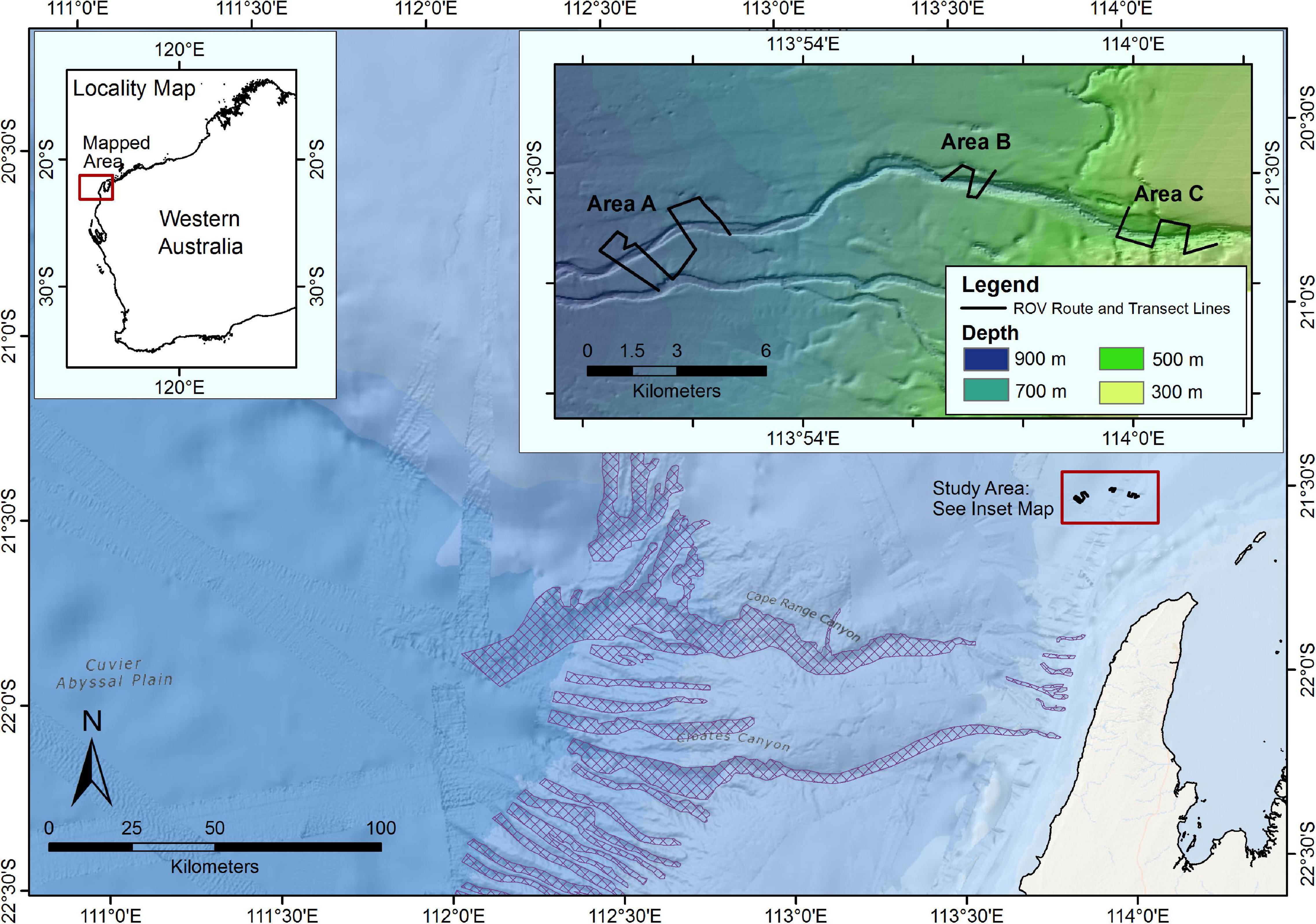
Figure 1. Context map illustrating the geographical location of the Greater Enfield survey area. Inset map illustrating the transect layout at each of the three survey Areas along a canyon-valley feature. Submarine canyons that are included in the Australian national submarine canyon database (Huang et al., 2014) are highlighted in cross-hatch (Source: Geoscience Australia).
Survey Method
The study was conducted over three consecutive days from 31 October to 2 November 2015. The survey was conducted using a Centurion QX 312 work class ROV fitted with stereo-video cameras to conduct transects with a standardised width of 5 m. A single downward facing video camera was used to simultaneously record benthic habitat. Water quality data (conductivity/salinity, temperature, and depth; CTD) was collected with a Sea-Bird Electronics (SBE) 19plus V2 SeaCAT Profiler CTD, mounted to the ROV platform. The ROV operated at approximately 1.5 m above the seabed and at a forward speed of approximately 0.5 knots. The total transect length covered by the ROV at Area A was approximately 11,330 m, Area B 3,470 m, and C 5,990 m.
The stereo-video system was made up of two Sony HDR CX550 handycams within custom built underwater housings with a depth rating to 2,000 m. The stereo-cameras were mounted onto a rigid base bar with a separation of 700 mm between the cameras and were inwardly converged at an angle of 8°, following the principles outlined by Harvey and Shortis (1995) and Goetze et al. (2019). This configuration provided an overlapping field of view from approximately 0.5 m in front of the cameras and accurate length measurements out to 8 m (Harvey et al., 2010). Stereo-video footage was recorded at high definition with a 1,920 × 1,080 resolution. A second stereo-video system was also fitted as redundancy in case of failure of the primary system. The stereo-video systems were mounted as low as possible onto the ROV (Figure 2), and camera systems were interfaced with and powered from the ROV systems. The ROV communication channels allowed the systems to be remotely controlled, and a live standard definition video stream from each camera was fed to the surface with live position, depth, date, and time overlays. To maximise illumination of the field of view, a combination of high output Light Emitting Diode (LED) and High Intensity Displacement (HID) lighting was used. These were placed as high as possible above the camera system on the ROV to reduce backscatter from suspended particles in the water column.
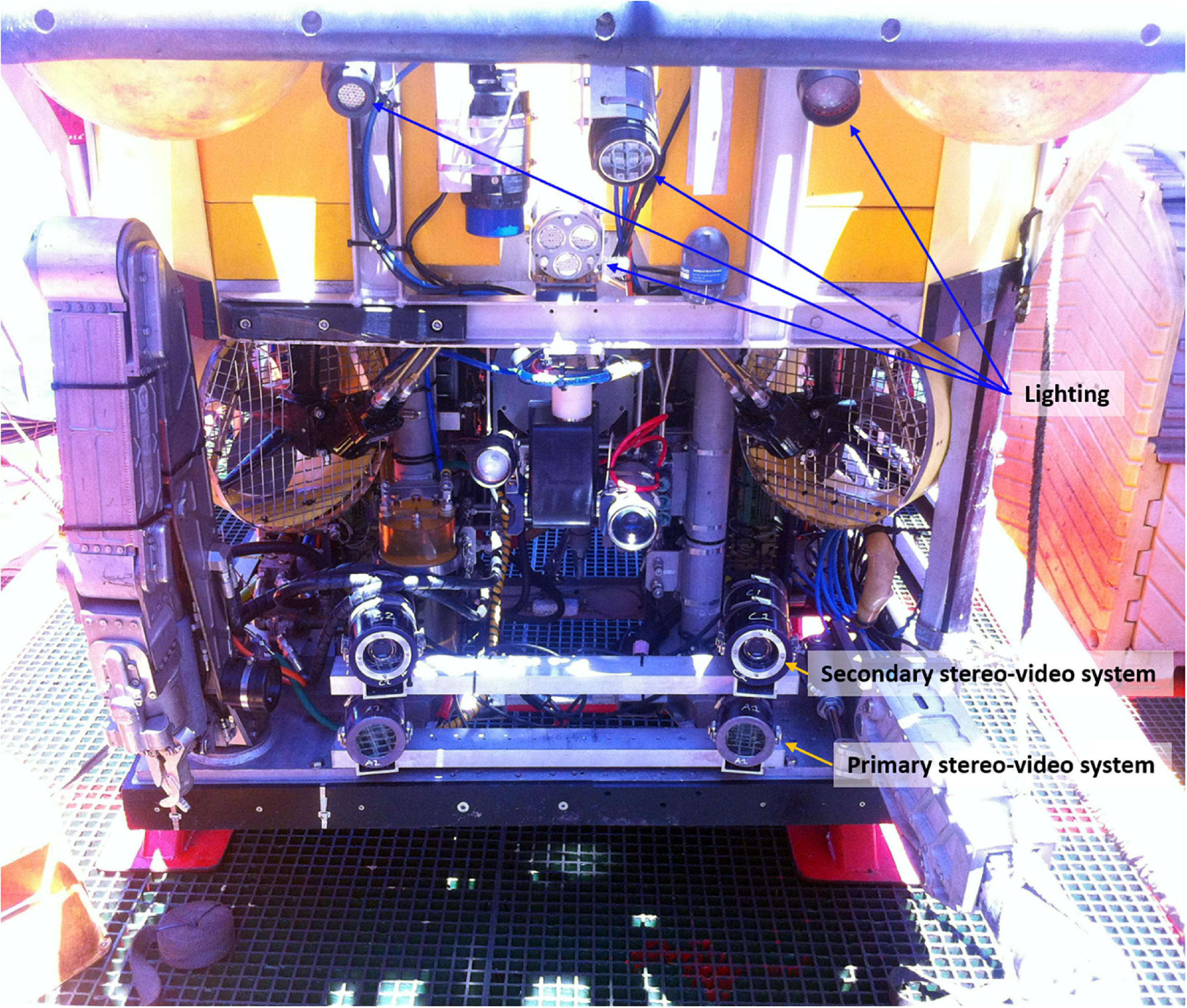
Figure 2. Front view of the QX312 ROV showing the position of the stereo-video camera systems and the lighting used during the survey. CTD was mounted to the rear of the ROV.
Identification of Taxa, Three Dimensional Positioning and Length Measurements
Video footage was analysed using EventMeasure Stereo software (SeaGIS, 2014). Identifications of fish were made by one experienced researcher based upon morphological features. In some cases, identification to species level was not possible as identifying features could not be distinguished on the video footage. In such cases, a precautionary approach was taken and taxa were identified to the lowest taxonomic resolution possible. Distinct taxa were given a unique number, which facilitated the assessment of diversity.
The calibrated stereo-video system (see Boutros et al., 2015) allowed accurate and precise measurements of the fork length (tip of nose to the middle caudal fin rays) of fishes, and the identification of the three dimensional position of each fish in relation to the ROV. To ensure fish were within the transect area (a 5 m belt), length measurements further than 2.5 m to either side or greater than 7 m in front of the ROV (based on the minimum visibility), were automatically rejected by the EventMeasure software.
Data Presentation and Statistical Analysis
The collection of data over transects of known position and dimensions allowed the use of two statistical approaches: Firstly, a multivariate analysis of variance approach was used to investigate differences in the fish assemblage structure between the three areas, and between canyon and non-canyon habitats. Secondly, a species distribution modelling approach was used to investigate environmental drivers of the distribution of taxa that were characteristic of each area, and to identify one taxa that was common and widely distributed over all three areas. These models were used to generate continuous predictive maps of the occurrence of these taxa over the survey areas.
Approach 1, Assemblage Patterns
Definition of canyon and non-canyon sections
Using bathymetry and slope data and the known depth profile of the ROV track log, transects were separated into two habitat types: canyon and non-canyon. Canyon habitats were defined as benthic habitat with increased depth, slope and structure, while the flat seabed surrounding the feature was classified as non-canyon habitat. Where a transect crossed over a canyon-valley habitat, the depth was noted outside of the canyon on both sides and the maximum depth inside the canyon-valley feature was also recorded (depths labelled A, B, and C, respectively, on Supplementary Figure 1.1). Taking a conservative approach and to avoid areas of transition between the two habitat types, a buffer section between canyon-valley and non-canyon was excluded from analyses. This buffer was calculated as 10% of the difference between the maximum canyon-valley depth and the depths outside the canyon-valley feature (C - A and C - B on Supplementary Figure 1.1). Video footage from the remaining depth of the canyon-valley feature (orange line in Supplementary Figure 1.1) was used to determine fish assemblage structure inside canyon-valley habitats.
Within each surveyed area (A, B, C), every time the transect crossed a canyon-valley feature, the video footage within the canyon-valley habitat was treated as a single replicate. As such, Area A had six replicate transect sections within canyon-valley habitat (Supplementary Figure 1.2), while Areas B and C both had five replicate transect sections within canyon-valley habitat (Supplementary Figure 1.2). To ensure comparability between habitats, similar replication occurred for non-canyon habitats such that Area A had six replicate transect sections and Area B had five. However, much of the area surveyed at Area C was steeply sloping and only two sections could be classified as non-canyon (Supplementary Figure 1.2; Supplementary Table 1.1).
Standardisation of data for assemblage analysis
To ensure that transect sections were statistically comparable, transect length and densities of fishes underwent three levels of standardisation prior to statistical analyses: Firstly, sections of transect were removed when the seabed was not within the field of view (Supplementary Figure 1.2). Secondly, the length of transects between canyon-valley and non-canyon habitats were standardised to one another. To achieve this, the total length of transect within each habitat was determined within each area, and then averaged. A note was taken of the habitat type with the shortest average transect length at each area. This shorter average length was then used to randomly select replicate segments of transects of that length in the other habitat in that area. If a transect section was shorter than the average length, its original length was used (Supplementary Table 1.1). Lastly, measures of fish assemblages from each transect section (as defined above) were standardised to a 250 m length by 5 m wide transect, or 1,250 m2. This transect length was used to increase the number of observations per transect for deep-sea fishes that are relatively sparse compared to shallower water fishes, but is similar to the length used other studies (Watson and Ormond, 1994; Newman et al., 1997; Westera et al., 2003). This allowed for fish assemblages within canyon-valley features of different sizes to be compared to each other and to non-canyon habitats. These standardised transects formed the replicates of the “canyon” and “non-canyon” levels within the factor “Habitats” in the statistical analysis design.
The fish assemblage abundance data and the total number of fish for each transect were standardised in this way. However, the number of taxa for each transect was not standardised to a 1,250 m2 transect area. This was to avoid artificially inflating the number of taxa observed in any transect. The influence of varying transect length on the number of taxa was assessed by including transect length as a covariate in the initial analysis. The interactions between transect length and the factors of Area and Habitat were not significant (all p > 0.20). Therefore we considered that transect length was not a confounding variable for tests of the number of taxa, and was not included in further statistical analysis.
Assemblage analysis approach
To investigate whether there were differences in the fish assemblage composition between the areas and habitats, a two-factor statistical design was used. The two factors tested were Areas (fixed factor, orthogonal; Area A vs. Area B vs. Area C) and Habitats (fixed factor, orthogonal; canyon vs. non-canyon). The standardised fish assemblage composition data was analysed using PERMANOVA (non-parametric analysis of variance; Anderson et al., 2008) add-in to the PRIMER v6 statistical software (Clarke and Gorley, 2006). The data were investigated for homogeneity of variance for the factors Habitat and Area using PERMDISP (permutational analysis of multivariate dispersions, Anderson, 2006). No taxa were numerically dominant and data was not transformed as the data met the assumption of homogeneity of variance. The multivariate fish assemblage composition was tested using PERMANOVA based upon a Bray Curtis similarity matrix. Number of taxa and the total number of fish were analysed separately using a univariate PERMANOVA based on a Euclidean distance resemblance matrix (Anderson, 2006; Clarke et al., 2006a,b). Where a significant difference (p < 0.05) was detected for the factor Area, post hoc tests were conducted to determine which of the Areas were significantly different.
To illustrate the multivariate patterns in the fish assemblage, a Principle Coordinate Ordination (PCO) was presented with vectors overlaid (Anderson et al., 2008). The vectors illustrate the strength and direction of the spearman rank correlation between the density of the taxa and the PCO axes. Taxa with a correlation stronger than 0.4 to either PCO axes were plotted. Results of the univariate analyses (number of taxa and total number of fish) were presented using bar graphs of means and standard error (SE).
Approach 2, Species Distribution Models
We developed individual Species Distribution Models (SDMs) for four fish taxa that were observed most frequently in the ROV videos. These models can help understand the ecology of these understudied taxa and map their environmental niche associations for future studies. The SDMs were developed using boosted regression trees (BRT) and “gbm” package applied in R software (R Core Team, 2014). BRT is a machine learning algorithm for additive numerical optimisation of the loss function to iteratively increase the predictive performance of the final model while gradually emphasising poorly modelled observations in the existing collection of trees (Elith et al., 2006). In the last decade, it has gained popularity within the marine spatial community because it is insensitive to outliers, missing data, or monotone transformations, and can be easily used with any type of predictors such as numeric, binary, categorical (Pittman et al., 2007; Oyafuso et al., 2017; Stamoulis et al., 2018). Fitted values in the final model are computed as the sum of all trees multiplied by the learning rate and are much more stable and accurate than those from a single decision tree model (Elith et al., 2006).
The occurrence data for each of the four taxa was extracted from direct observations of each occurrence from the underwater video recording along the ROV tracks and were using in BRT fitting as records of taxa presence. As BRT models also require a sample of observations to characterise the available environment to discriminate used from available habitat (pseudo-absences, Boyce et al., 2002; Phillips et al., 2009; Franklin, 2010) we derived pseudo-absences for all taxa by randomly sampling all the available data points along the ROV tracks where the study taxa were not recorded. Because presence records for all study taxa were low, we created a final ratio of 1:1 of the observed presences and pseudo-absences of each study taxa along the tracks to effectively estimate unbiased parameters for rare populations (Fielding and Bell, 1997; Franklin, 2010; Galaiduk et al., 2017b). The final datasets were partitioned into training (75%) and testing (25%) data for individual modelled taxa and tested for spatial autocorrelation between observations. The explanatory variables were a set of 9 functionally relevant environmental predictors with Spearman’s rank correlation between them <0.7 which is considered to be acceptable for spatial models (Moore et al., 2011; Galaiduk et al., 2017a; Table 1) that describe the structure, complexity and type of benthic habitat derived from the bathymetry data using Spatial Analyst toolkit in ArcGIS 10.3. The 10th variable, “Habitat type,” was categorical, and described occurrence of benthic biota and signs of bioturbation. This was derived through unsupervised classification procedures in ERDAS using direct observation along the ROV transects and post processed with the Spatial Analyst toolkit in ArcGIS (Table 1).
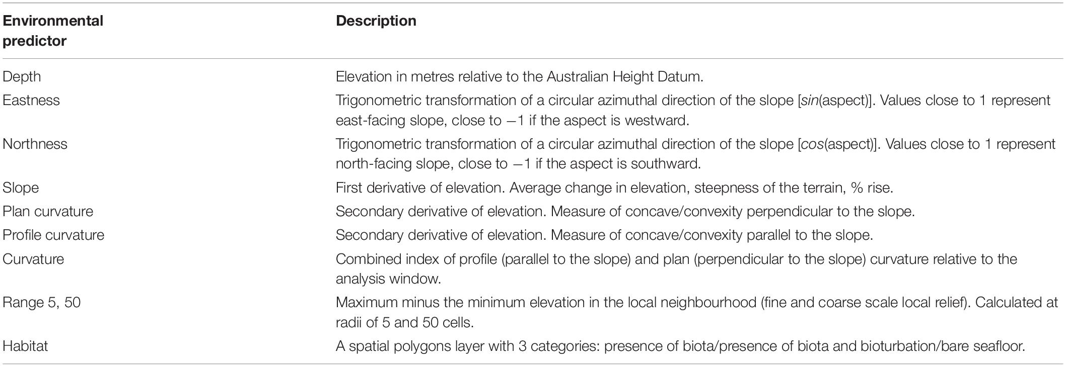
Table 1. Summary of the environmental predictors extracted from the hydroacoustic survey used for fitting boosted regression trees.
To determine the effect of environmental predictors and their importance on the probability of occurrence of four fish taxa, we fitted BRT models on training datasets for these taxa following the procedures outlined in Elith et al. (2008). Optimal model settings were chosen using 10-fold cross-validation by optimising learning rate, bagging rate and tree complexity (Leathwick et al., 2006). The optimal model was considered a model that produced the lowest cross-validated residual deviance with at least 1,000 fitted trees. Selected models were then simplified to remove less informative predictors which achieved more parsimonious models without degradation of model fits (Elith et al., 2008). The importance of predictor variables in the simplified BRT models was determined using the variable importance score based on the improvements of all splits associated with a given variable across all trees when this variable was added in the model (Leathwick et al., 2006).
To assess the predictive performance, and discrimination and accuracy of fitted models, a set of common evaluation metrics of predictive performance was calculated on the test datasets. We used Receiver Operating Characteristic (ROC) and the area under the curve (AUC) as graphical means to test the sensitivity (true positive rate) and specificity (false positive rate) of a model output (Fielding and Bell, 1997). The AUC is a measure of the ability of a model to discriminate between a presence or absence observation (Elith et al., 2006). In addition, we calculated a threshold dependent Kappa statistic which is commonly used in ecological studies with presence-absence data and provides an index between 0 and 1 of how much a model predicted actual classes versus a guess (Cohen, 1960). A probability threshold that balances sensitivity and specificity was chosen as it provides a measure of how well the model predicts both presences and absences (Liu et al., 2005). After evaluation, the final models for individual taxa were predicted on 4 × 4 m grid using all available observations.
Results
Oceanographic Situation
The CTD profiles revealed a steady decline in water temperature with depth across all Areas, from ∼25°C at the surface to ∼6°C at the deepest point (∼800 m) (Figure 3A). Salinity increased from ∼35 ppt at the surface to a maximum of ∼35.5 ppt at ∼150–200 m, and then decreased to a minimum of ∼34.6 ppt at depths greater than ∼500 m across all three surveyed Areas (Figure 3A).
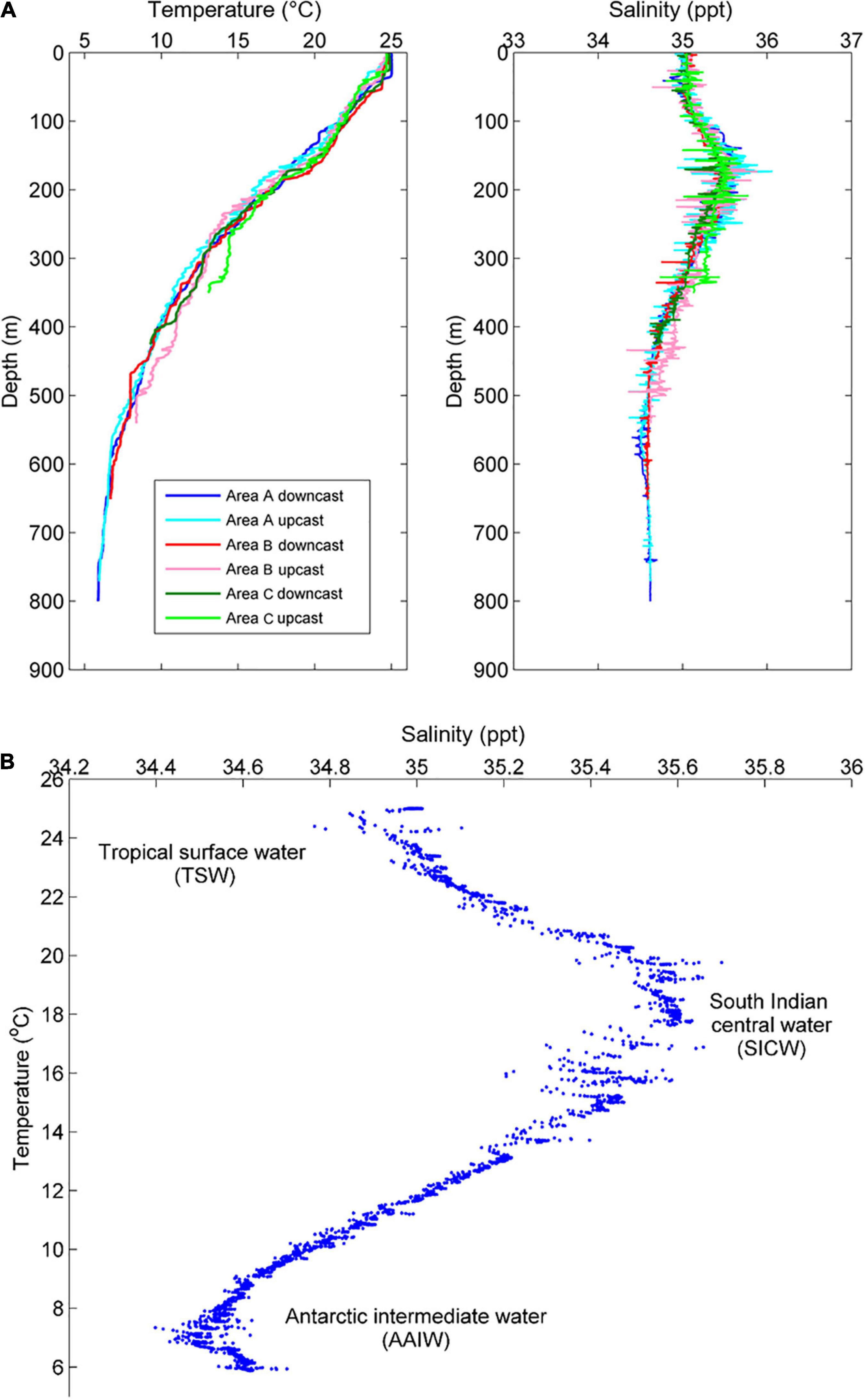
Figure 3. (A) Vertical profiles of temperature and salinity across all Areas, and (B) temperature-salinity measured on the downcast at Area A.
The relationship between temperature and salinity (T-S plot; Figure 3B) at the deepest site (Area A) was used to evaluate the localised water masses, with reference to recent evaluations of deep-water hydrography off the Gascoyne region (Woo and Pattiaratchi, 2008). Based on the analyses of Woo and Pattiaratchi (2008), three water masses were identified. Firstly, a lower salinity tropical surface water (TSW) with a temperature range of ∼22–25°C was found in the upper ∼100 m of water column. Secondly, a higher salinity South Indian Central Water (SICW) with a temperature range of 12–22°C was centred on ∼200 m depth. Lastly, a lower salinity Antarctic Intermediate Water (AAIW) with a temperature range of ∼6–9°C was identified ∼550 m depth.
Near-bottom time series profile from Area A (depths ∼800–875 m) showed a temperature range of ∼5.7–6.3°C and relatively uniform salinity (∼34.6; Figure 4). At Area B, near-bottom (∼560–680 m) temperatures ranged ∼6.6–7.8°C and salinity was relatively uniform (∼34.6; Figure 4). The shallowest transect (∼350–560 m) in Area C showed a temperature range of ∼6.7–13°C and a salinity range of ∼34.6–35.1 (Figure 4). In general, the coldest, most dense water was found as the ROV traversed the deepest portions of the canyon-valley features.
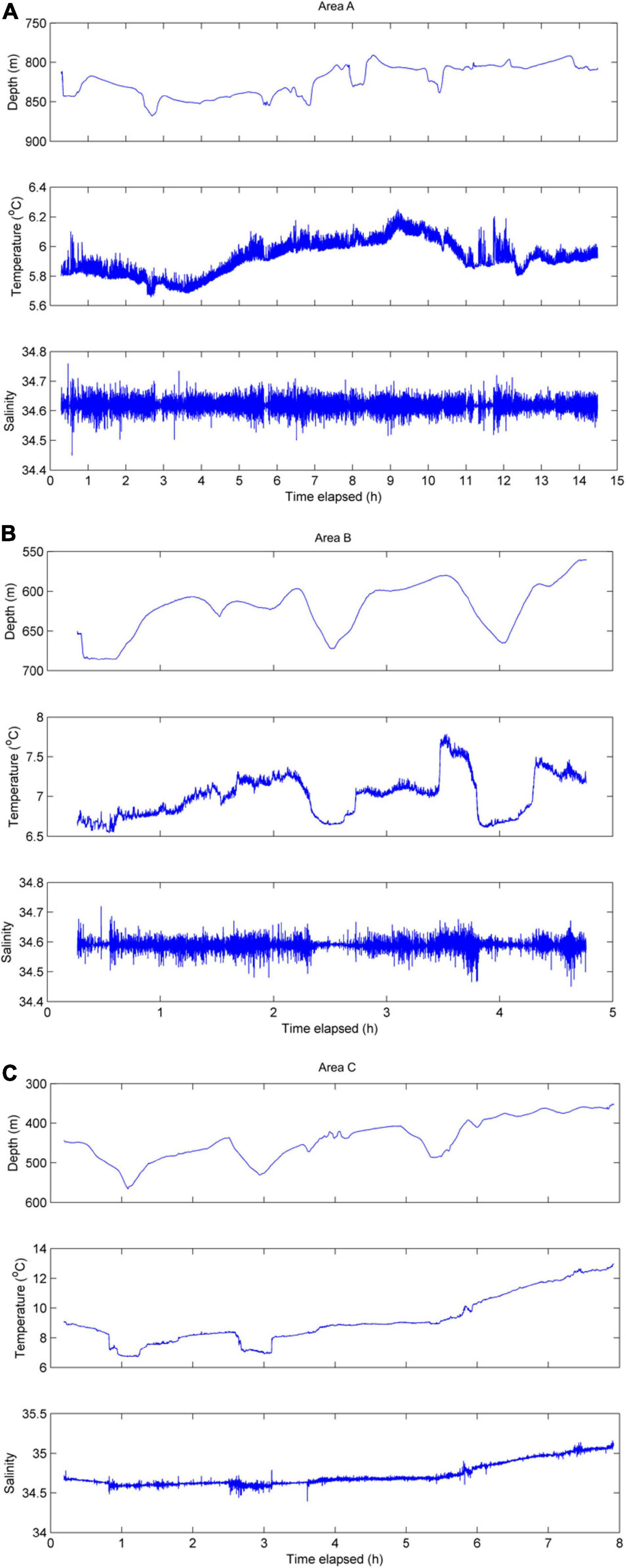
Figure 4. Time series of near-bottom data collected along Area A transect (A), Area B transect (B), and Area C transect (C).
General Description of Fish Assemblages
Across the three areas surveyed, the total transect length was ∼20,790 m giving a total transect area of 103,950 m2 or 10.4 hectares. Along the entire transect, a total of 610 individual fish were recorded belonging to 80 unique taxa and 41 families. A full list of the taxa recorded by area, the total number of each taxa and their mean lengths are shown in Supplementary Table 1.2. Many of the taxa and individual fish recorded were small bodied (<30 cm fork length; Supplementary Table 1.2), however, a large 63 cm morid cod (Moridae sp3), was recorded, along with a number of larger bodied elasmobranchs. A 1.3 m whaler shark (Carcharhinus sp1) was the largest elasmobranch identified. The western gulper shark (Centrophorus westraliensis) had the largest mean fork length (86 ± 2.5 cm SE). The indigo legskate (Sinobatis caerulea) was the second largest taxa recorded on average at 74 ± 11.3 cm disc length (excluding the tail). One large 71 cm Chimaera Hydrolagus lemures (blackfin ghost shark) was also measured (Supplementary Table 1.2).
Approach 1, Assemblage Analysis
For total number of fish, a significant difference was found (at α = 0.05) between Areas and between Habitats, but there was no interaction between the two factors (Table 2). On average, the greatest number of fish per transect (1,250 m2) was recorded at Area B (Figure 5; Area B vs. Area A t(18) = 2.56, p = 0.003, Area B vs. Area C t(12) = 2.20, p = 0.04). The total number of fish recorded per transect were similar at Areas A and C (Figure 5, t(14) = 1.59, p = 0.134). On average, a significantly greater number of fish were recorded in canyon-valley Habitats compared to non-canyon Habitats (Table 2; Figure 5). Canyon-valley Habitats were also found to support a significantly greater number of taxa on average than non-canyon Habitats (Table 2; Figure 5). No significant difference was found in number of taxa between the survey Areas (Table 2), although the composition of the assemblages did vary.
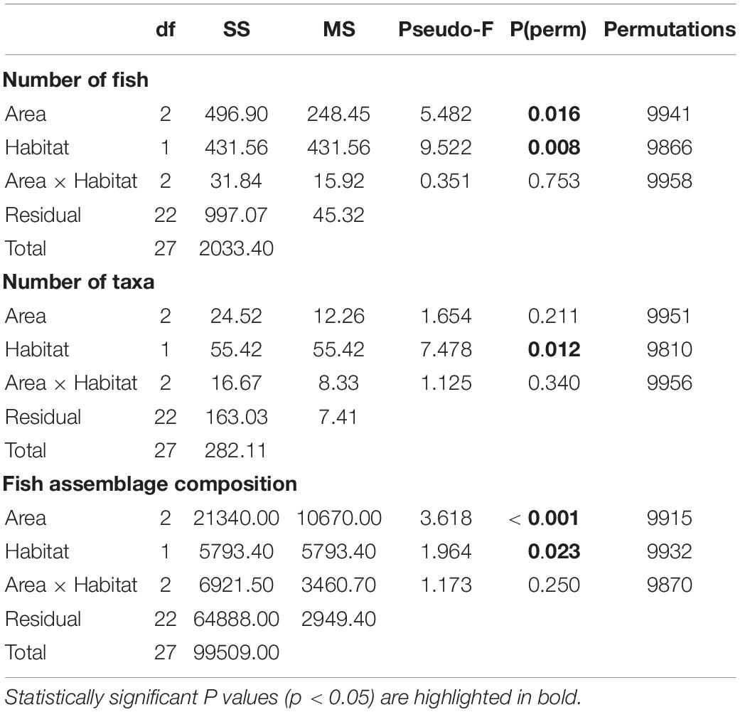
Table 2. PERMANOVA test results for the statistical analysis of the fish assemblage composition between Areas (A, B, C) and Habitat (canyon, non-canyon).
Figure 5. The mean ± SE of (A) number of fish recorded (1,250 m– 2) at each Area, (B) the number of fish recorded (1,250 m– 2) in each Habitat, and (C) number of taxa recorded (transect−1) in each Habitat.
Significant differences in the multivariate fish assemblage composition were found between both Areas and Habitats, but no interaction between these factors (Table 2). Post hoc tests on the factor Area revealed that all Areas differed to one another (all t > 1.14, all p < 0.03). The multivariate PCO showed three distinct groupings (Figure 6). The PCO shows transects at Area A clustered to the left of the plot were correlated to unidentified anguilliform (eel-like) fishes, and Paraliparis sp1 (a snail fish), as both fish were abundant in this area. In comparison, Paraliparis sp1 made up only 2% of the individuals recorded at Area B and were absent at Area C (Supplementary Table 1.2). Samples to the right side of the PCO plot are arranged into two clusters (Figure 6). The bottom grouping is characterised by four Macrouridae (rat tail) taxa which were characteristic of Areas B and C. The grouping toward the upper right side of the plot is characterised by a mixed grouping of taxa. Chaunax sp1 (a coffin fish) were more abundant at both Areas B and C than at Area A. Ariosoma sp1 (a conger eel), Coelorinchus sp1 (a rat tail), and Moridae sp2 (a morid cod) were recorded only at Area B (Supplementary Table 1.2). One sample from Area C is grouped to the left of the plot with Area A samples. This transect contained a single fish, an unidentified anguilliform fish.
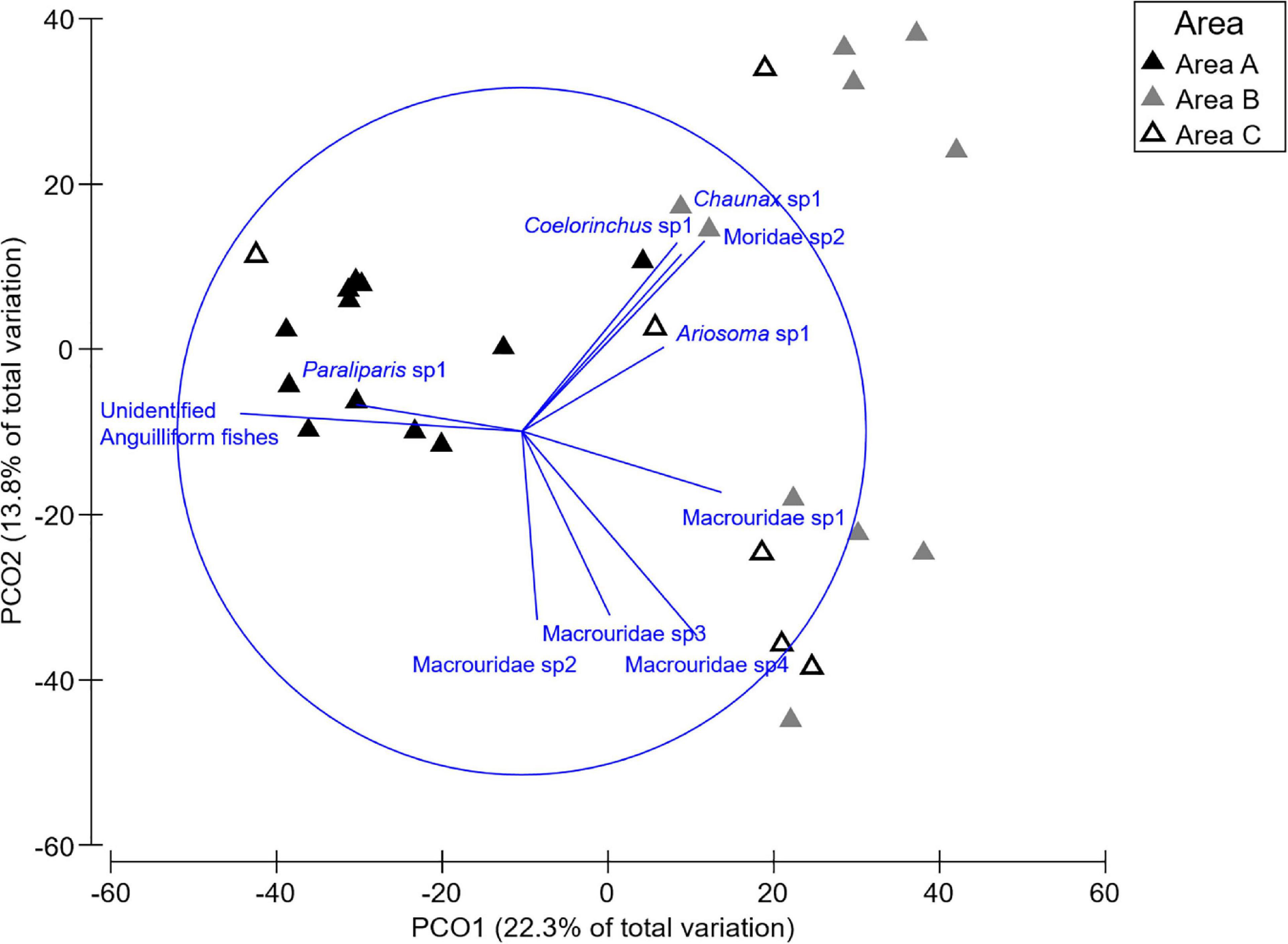
Figure 6. Principle component ordination (PCO) illustrating the variation between transects by Area. The overlaid vectors illustrate the strength and the direction of the correlation to the PCO axes of influential fish species.
Approach 2, Species Distribution Models
Model Performance
Boosted regression trees models provided “good” model predictions (AUC = 0.80–0.89) for two taxa and “poor” predictions (AUC = 0.60–0.69; Table 3) for the other two taxa according to the criteria of Hosmer et al. (2013). Similar trends in the performance of fitted models were evident for all the other evaluation metrics with sensitivity, specificity and the total proportion of correct predictions being highest for the Macrouridae sp5 and Paraliparis sp1. These performance measures were further corroborated by Kappa statistics with models for Macrouridae sp2 and Macrouridae sp4 performing “fair” (Kappa = 0.21–0.40) and models developed for Macrouridae sp5 and Paraliparis sp1 providing “substantial” (Kappa = 0.61–0.80; Table 3) predictions (Landis and Koch, 1977).
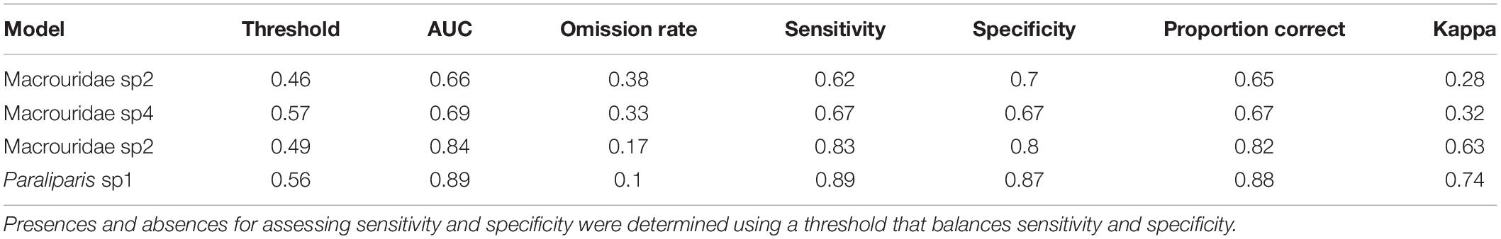
Table 3. Summary of model predictive performance for each fish species.
Habitat Associations
Depth had the greatest influence on the probability of occurrence of all taxa (Figure 7). For Macrouridae sp2, Macrouridae sp5 and Paraliparis sp1, higher probability of occurrence was associated with water depth over 600 m. In contrast, Macrouridae sp4 was predicted to be most likely to occur at depths between 500 and 600 m (Figure 7). Various indices of topographic complexity of the relief (plan, profile, curvature and range 50) were also important in influencing the probability of occurrence of Macrouridae sp2, Macrouridae sp4 and Macrouridae sp5. Higher probability of occurrence of Macrouridae sp2 and Macrouridae sp4 was predicted on the seabed surrounding the canyon-valley slopes, whereas Macrouridae sp5 was predicted to be deeper and associated with both flat areas of low structural complexity, and within the feature on canyon-valley slopes and the canyon floor (Figures 7, 8). A higher probability of occurrence of Paraliparis sp1 was predicted on deep non-canyon habitats (Figures 7, 8).
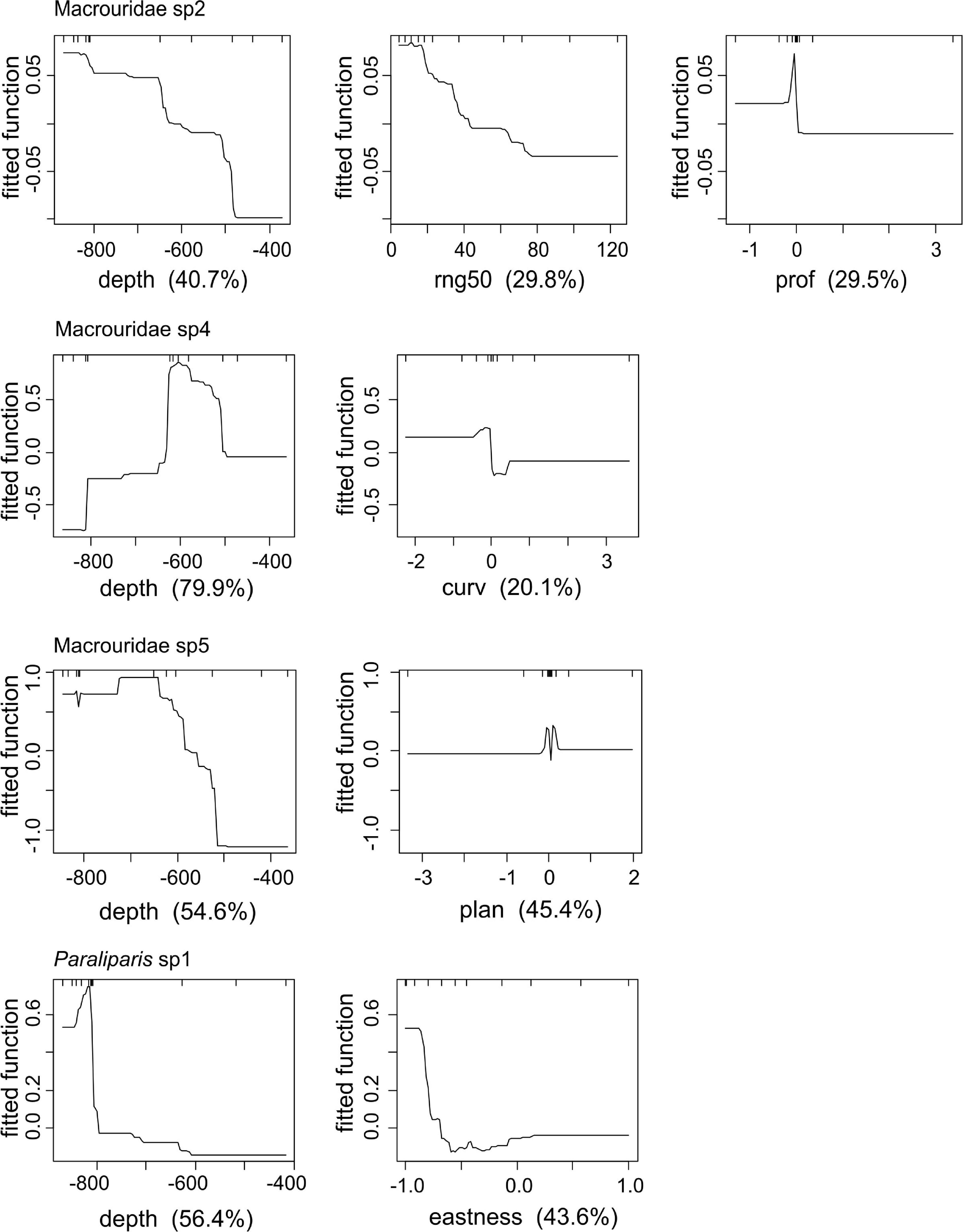
Figure 7. Partial dependence plots for Boosted Regression Tree (BRT) analyses relating species occurrence to the environmental predictors. The relative importance of each variable is shown in parentheses on the x-axis.
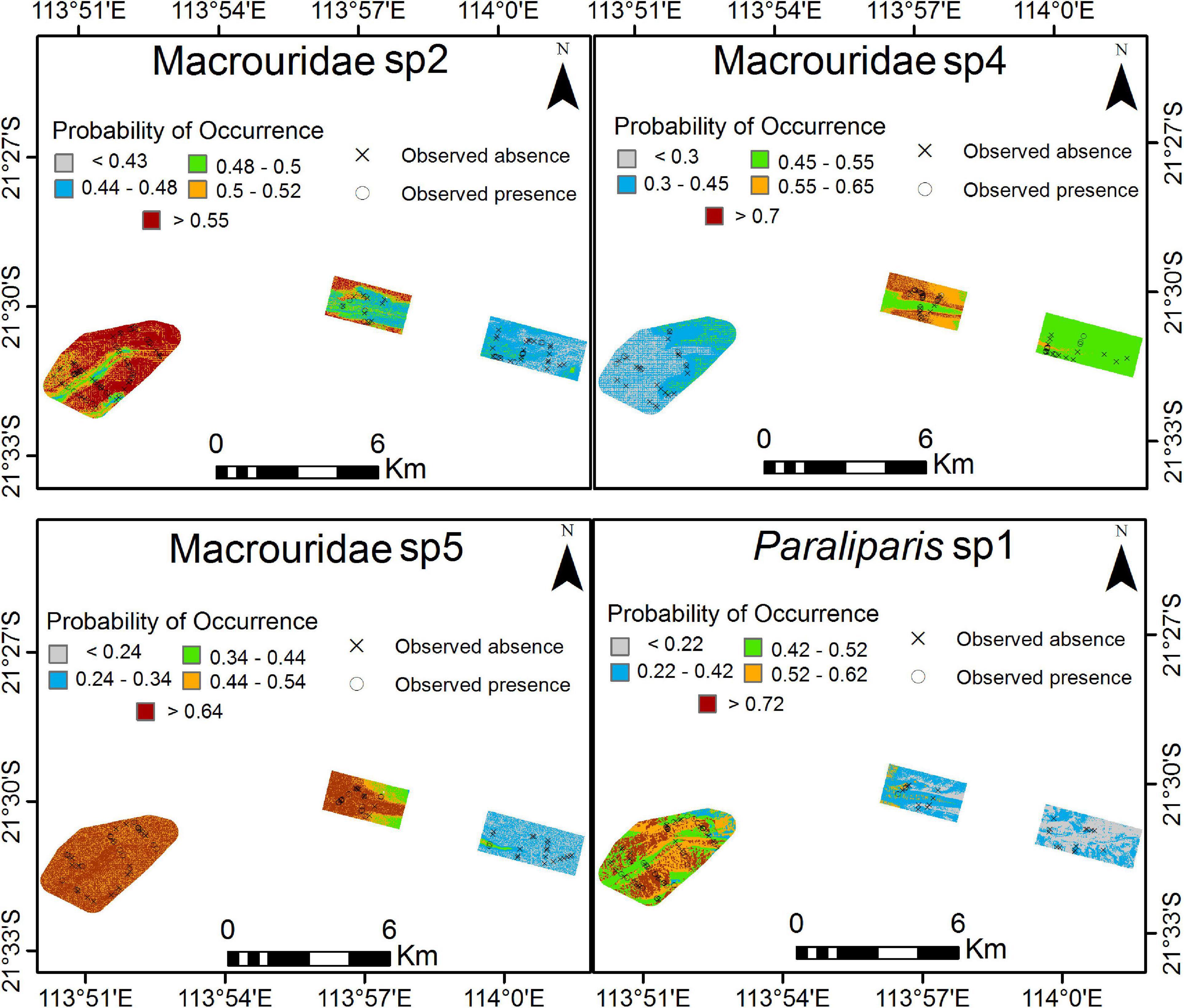
Figure 8. Predicted probability of occurrence for each species across 3 Areas as a result of Boosted Regression Trees analysis. Higher probability of occurrence is in red. For high resolution images please see Supplementary Materials 2 through 5.
Spatial Patterns of Distributions
A high probability of occurrence of Macrouridae sp2, Paraliparis sp1 and Macrouridae sp5 was predicted in the deepest area A (Figure 8; Supplementary Material 2, 3, 5). A high probability of occurrence of Macrouridae sp5 was predicted in Area A, and also over the deeper areas (>500 m) and within the canyon-valley of Area B. In contrast, higher probability of occurrence of Macrouridae sp2 and Macrouridae sp4 in area B was predicted for regions outside the canyon-valley and on its slopes, respectively (Figure 8). Macrouridae sp4 was also predicted to occur within the deeper canyon-valley of Area C and the shallower regions of Area A, reflecting its predicted relationship with depth (Figure 8; Supplementary Material 4).
Discussion
Deep-water environments and subsea canyons support diverse fish assemblages which are different to nearby shallow water assemblages (Williams et al., 2001; Fernandez-Arcaya et al., 2017). Here, we combined novel survey methods and advanced analytical approaches to document patterns of deep-water fish assemblage composition and spatial distributions. We also showed that subsea canyon environments support fish assemblages characterised by a higher number of taxa and overall number of individuals when compared to the areas outside the canyon, which likely reflects the heterogeneity of habitat and oceanographic conditions within the canyon (Klinck, 1996; McClain and Barry, 2010). A combination of non-extractive survey methods and SDMs provided a useful tool for improving our understanding of fine-scale spatial distribution patterns of deep-water fishes and the associated environmental drivers.
The survey area had a high diversity of taxa for a deep-sea environment with 80 taxa of fish from 41 families recorded, which is consistent with previous observations of fish diversity in this region (Williams et al., 1996, 2001). The family Macrouridae (rat tails) dominated the fish assemblage across the survey area, which is also supported by earlier research (Williams et al., 1996, 2001). We recorded 11 Macrouridae taxa whereas Williams et al. (1996) reported 16 species of Macrouridae using trawls within the same latitudinal and depth range (21–22°S, 300–900 m depth). There was a consistent pattern between areas in that the canyon-valley features supported a greater number of fish and a higher diversity of taxa than non-canyon habitat. This is likely due to variation in the habitat structure of the canyon-valley feature (McClain and Barry, 2010). At Areas A and B, the canyon-valley habitat was wide (250–500 m) and topographically shallow (20–50 m) in comparison to Area C which was a more typical canyon feature. Submarine canyon habitats can support higher abundances of benthic feeding fishes than nearby continental shelf slopes (De Leo et al., 2010). Greater prey availability in sediment infauna and epifauna may support the increased abundance of fishes, particularly Macrouridae, which were characteristic of canyon-valley habitats (De Leo et al., 2010).
A different fauna characterised the deeper Area A compared to Areas B and C. This was likely to be due to the influence of the AAIW deep water current at area A. Submarine canyons are important in linking continental slope and shelf areas and water masses. Canyon features change nutrient dynamics through increased upwelling and interactions with alongshore currents (Klinck, 1996), and are important for supplying nutrients to deep ocean through down-canyon transport (Fernandez-Arcaya et al., 2017). Area A was differentiated from Areas B and C by a higher abundance of the species group of unidentified anguilliform fishes and also a higher abundance of Paraliparis sp1 (a snail fish). Species from the genus Paraliparis generally inhabit the deep sea, and have been recorded in this region at depths of 1,030 m (Williams et al., 1996), and 2,821 m in New Zealand (Roberts et al., 2015). A similar pattern of a faunal break between fish assemblages on the upper and the mid-slope was reported by Last et al. (2011), which can be attributed to the influence of the AAIW (Williams et al., 2001). This deep-water current has a significant influence on the distribution of fish communities in the south-west region between the Great Australian Bight and north of the Ningaloo Reef where its core is known to fluctuate with depth from approximately 875 m at 27.50°S to 520 m around 21.50°S (Williams et al., 1996, 2001; Woo and Pattiaratchi, 2008). A full assessment of the influence of this current on fish assemblages within our study area would require further specifically targetted research.
Our study contributes additional information to understanding fish communities and their relationship to benthic habitats in two KEFs for the Australian northwest marine region; Canyons linking the Cuvier Abyssal Plain and the Cape Range Peninsula and Continental Slope Demersal Fish Communities (DSEWPaC, 2012). Deep-sea KEFs are often data-poor and their definition is often based on limited data (Falkner et al., 2009). The Canyons linking the Cuvier Abyssal Plain and the Cape Range Peninsula are representative features of the region but are not unique in a wider Australian context (Falkner et al., 2009). In terms of the Continental Slope Demersal Fish Communities KEF, Last et al. (2005) recorded 500 species making it the most biodiverse slope region in Australia. In comparison, we recorded 80 taxa, but our study focus was on a tributary to a canyon system, and not the entire continental slope assessed by Last et al. (2005).
We elucidated the distribution patterns of the four most abundant taxa within the assemblages using SDMs. SDMs are a useful tool for exploring habitat associations of the deep-sea fishes because they provide insights into the ecology of these rarely observed taxa and data can be extrapolated into unsurveyed areas. Often depth and habitat complexity drive environmental niche associations of demersal fishes (Monk et al., 2010; Moore et al., 2013; Galaiduk et al., 2018). This was observed in our study, where depth was the most important environmental predictor for all modelled taxa. Our models identified Paraliparis sp1 to be primarily associated with water depth over 800 m. In contrast, the three other taxa were predicted to occur at water depth greater than 500 m with Macrouridae sp4 predicted to mainly occupy depths between 500 and 600 m. Habitat complexity calculated at different scales was also an important predictor of habitat associations of the modelled taxa, suggesting that these taxa use various sized nooks and crevices (as estimated from the bathymetry derivatives) for shelter and protection from predation (Kelley et al., 2006). Macrouridae sp2 and Macrouridae sp4 were predicted to occupy the canyon slopes, whereas Macrouridae sp5 was predicted to be more associated with areas within the canyon and the canyon floor, suggesting within-family partitioning of the available environmental niche space to avoid resource overlap (Ross, 1986).
Biological data collection in deep-sea environments is expensive and labour-intensive. Large vessels capable of deploying multiple data collection platforms (e.g., ROVs, CTD probes, sediment corers, and camera systems) through the water column to the seabed, often to depths of 1,000’s of metres, are required (McLean et al., 2020). In this study, we streamlined the collection of multiple data types simultaneously (stereo-video imagery of fishes, benthic habitat imagery, and CTD) by deploying multiple instruments on a single ROV platform. This efficient configuration is recommended for future environmental studies of both shallow and deep seas as it minimises the time required to collect data. The methods are particularly applicable to baseline studies that support environmental impact assessments for offshore facilities (e.g., oil and gas) and inform the planning and management of marine reserves.
Remotely Operated Vehicle operated surveys are an industry-supported method with potential for large data collection in remote marine environments rarely accessible to researchers (McLean et al., 2017, 2018a; Macreadie et al., 2018). ROVs present a platform which can be fitted with multiple tools to collect a variety of environmental data from challenging remote environments (McLean et al., 2017, 2018a; Macreadie et al., 2018). Previously, sampling has relied on extractive trawls, or more recently deep-water baited cameras (Priede and Bagley, 2000; Jamieson et al., 2009; Marouchos et al., 2011; Wellington et al., 2021). These techniques are better suited to describing broader-scale spatial patterns (100 s of m) than the fine-scale sampling (<10 s of m) using the transect and SDM approach described in this study. The ROV transect approach allows for the in situ observation of fishes (Macreadie et al., 2018), and the investigation of fine-scale fish-habitat relationships through SDMs. It also eliminates the bias associated with the use of baited video systems (i.e., the bait plume effect; see Galaiduk et al. (2017b) and Monk et al. (2012) for a comparison between methods and applications in SDMs).
The ROV, however, has its own biases associated with noise, and the bright lighting required to collect quality video footage in dark environments which may affect the behaviour of mobile fauna (Ryer et al., 2009). We did not observe adverse behavioural reactions or fleeing, however, it is possible that certain taxa may simply avoid the ROV entirely and were thus not recorded (Linley et al., 2013). It is likely that avoidance by mobile fauna is greatest over soft sediment habitats such as those sampled during this study (Schramm et al., 2020a). These artefacts and avoidance may have implications for SDMs, however, they were consistent throughout the survey and should not affect statistical comparisons between Habitats or Areas. Traditional extractive methods for sampling deep-sea environments have biases and limitations relating to the gear and the spatial resolution of samples obtained. Previous studies from the region used a large netted paired-warp trawl rig (Williams et al., 1996, 2001) that may have under-sampled small species (Williams et al., 2001). Smaller meshed nets used in this region have caught a different suite of fishes, including more Ophidiidae (cusk eels) and Congridae (conger eels) (Williams et al., 2001). Many of the fishes measured during our ROV survey were between 10 and 30 cm in length, and so may have been under represented in previous trawl surveys. Similarly, in our stereo-video ROV survey the positive identification of many small bodied (<10 cm) individuals was difficult because morphological features were indistinct. Therefore, both stereo-video ROV and trawl methods may under sample the diversity of small bodied fishes.
Conclusion
The submarine canyon-valley feature sampled here supports a characteristically rich fish assemblage with a greater number of taxa and individuals than areas outside the feature. This canyon-valley feature is a tributary to the larger Cape Range canyon system which may play an ecological role in linking the Cuvier Abyssal Plain and the Cape Range Peninsula (Huang et al., 2018). Here, we present a novel application of ROV stereo-video transects in deep water, demonstrating the utility of this technique for facilitating fine-scale fish species distribution modelling that has the potential to feed into spatial management of deeper offshore waters.
Data Availability Statement
The datasets presented in this article are not readily available because the data are commercial in confidence. Requests to access the datasets should be directed to environment@bmtglobal.com.
Ethics Statement
Ethical review and approval was not required for the animal study because at the time that the study was conducted ethical review and approval was not required for observational studies.
Author Contributions
BS, EH, LT, MW, KI, and DM conceived and designed the study. BS, KI, and LT collected the data. BS, RG, and KI analysed the data. BS, RG, EM, JG, and KI developed the initial version of the manuscript. All authors contributed to interpreting the data and developing the full manuscript.
Funding
This research was supported by funding and data from the Woodside-operated Greater Enfield Project, a Joint Venture between Woodside Energy Ltd. and Mitsui E&P Australia Pty Ltd.
Conflict of Interest
KI, MW, and LT was employed by the company BMT Commercial Australia. DM was employed by the company Woodside Energy Ltd.
The remaining authors declare that the research was conducted in the absence of any commercial or financial relationships that could be construed as a potential conflict of interest.
Publisher’s Note
All claims expressed in this article are solely those of the authors and do not necessarily represent those of their affiliated organizations, or those of the publisher, the editors and the reviewers. Any product that may be evaluated in this article, or claim that may be made by its manufacturer, is not guaranteed or endorsed by the publisher.
Supplementary Material
The Supplementary Material for this article can be found online at: https://www.frontiersin.org/articles/10.3389/fmars.2021.608665/full#supplementary-material
References
Adams, P. B., Butler, J. L., Baxter, C. H., Laidig, T. E., Dahlin, K. A., and Waldo Wakefield, W. (1995). Population estimates of Pacific coast groundfishes from video transects and swept-area trawls. Fish. Bull. 93, 446–455.
Agapova, G. V., Budanova, L. Y., Zenkevich, N. L., Larina, N. I., Litvin, V. M., Marova, N. A., et al. (1979). Geomorphology of the ocean floor, Geofizika okeana. Moscow: Geofizika okeanskogo dna, Neprochnov, Izd.
Anderson, M. J. (2006). Distance-based tests for homogeneity of multivariate dispersions. Biometrics 62, 245–253. doi: 10.1111/j.1541-0420.2005.00440.x
Anderson, M. J., Gorley, R. N., and Clarke, K. R. (2008). PERMANOVA+ for PRIMER: Guide for Software and Statistical Methods. Plymouth: University of Auckland and Plymouth Marine Laboratory.
Appeltans, W., Ahyong, S. T., Anderson, G., Angel, M. V., Artois, T., Bailly, N., et al. (2012). The magnitude of global marine species diversity. Curr. Biol. 22, 2189–2202.
Armstrong, C. W., Foley, N. S., Tinch, R., and van den Hove, S. (2012). Services from the deep: Steps towards valuation of deep sea goods and services. Ecosyst. Serv. 2, 2–13. doi: 10.1016/j.ecoser.2012.07.001
Bo, M., Bava, S., Canese, S., Angiolillo, M., Cattaneo-Vietti, R., and Bavestrello, G. (2014). Fishing impact on deep Mediterranean rocky habitats as revealed by ROV investigation. Biol. Conserv. 171, 167–176. doi: 10.1016/j.biocon.2014.01.011
Bond, T., Partridge, J. C., Taylor, M. D., Cooper, T. F., and McLean, D. L. (2018). The influence of depth and a subsea pipeline on fish assemblages and commercially fished species. PLoS One 13:e0207703.
Boutros, N., Shortis, M. R., and Harvey, E. S. (2015). A comparison of calibration methods and system configurations of underwater stereo-video systems for applications in marine ecology. Limnol. Oceanogr. Methods 13, 224–236. doi: 10.1002/lom3.10020
Boyce, M. S., Vernier, P. R., Nielsen, S. E., and Schmiegelow, F. K. (2002). Evaluating resource selection functions. Ecolog. Model. 157, 281–300. doi: 10.1016/s0304-3800(02)00200-4
Cappo, M., Speare, P., and De’ath, G. (2004). Comparison of baited remote underwater video stations (BRUVS) and prawn (shrimp) trawls for assessments of fish biodiversity in inter-reefal areas of the Great Barrier Reef Marine Park. J. Exp. Mar. Bio. Ecol. 302, 123–152. doi: 10.1016/j.jembe.2003.10.006
Clark, M. (2001). Are deepwater fisheries sustainable?—the example of orange roughy (Hoplostethus atlanticus) in New Zealand. Fish. Res. 51, 123–135. doi: 10.1016/s0165-7836(01)00240-5
Clarke, K. R., Chapman, M. G., Somerfield, P. J., and Needham, H. R. (2006a). Dispersion-based weighting of species counts in assemblage analyses. Mar. Ecol. Prog. Ser. 320, 11–27. doi: 10.3354/meps320011
Clarke, K. R., Somerfield, P. J., and Chapman, M. G. (2006b). On resemblance measures for ecological studies, including taxonomic dissimilarities and a zero-adjusted Bray–Curtis coefficient for denuded assemblages. J. Exp. Mar. Biol. Ecol. 330, 55–80. doi: 10.1016/j.jembe.2005.12.017
Cohen, J. (1960). A coefficient of agreement for nominal scales. Educ. Psychol. Meas. 20, 37–46. doi: 10.1177/001316446002000104
Cruz-Acevedo, E., Tolimieri, N., and Aguirre-Villaseñor, H. (2018). Deep-sea fish assemblages (300-2100 m) in the eastern Pacific off northern Mexico. Mar. Ecol. Prog. Ser. 592, 225–242. doi: 10.3354/meps12502
Danovaro, R., Snelgrove, P. V. R., and Tyler, P. (2014). Challenging the paradigms of deep-sea ecology. Trends Ecol. Evol. 29, 465–475. doi: 10.1016/j.tree.2014.06.002
De Leo, F. C., Smith, C. R., Rowden, A. A., Bowden, D. A., and Clark, M. R. (2010). Submarine canyons: hotspots of benthic biomass and productivity in the deep sea. P. Roy. Soc. B-Biol. Sci. 277, 2783–2792. doi: 10.1098/rspb.2010.0462
DSEWPaC. (2012). Marine bioregional plan for the North-West Marine Region prepared under the Environment Protection and Biodiversity Conservation Act 1999. Canberra: Australian Government Department of Sustainability Environment Water Populations and Communities.
Elith, J., Graham, C. H., Anderson, R. P., Dudík, M., Ferrier, S., Guisan, A., et al. (2006). Novel methods improve prediction of species’ distributions from occurrence data. Ecography 29, 129–151.
Elith, J., Leathwick, J. R., and Hastie, T. (2008). A working guide to boosted regression trees. J. Animal Ecology 77, 802–813.
Falkner, I., Whiteway, T., Przeslawski, R., and Heap, A. D. (2009). Review of Ten Key Ecological Features (KEFs) in the North-west Marine Region. Geoscience Australia, Record 2009/13. Canberra: Geoscience Australia, 117.
Fernandez-Arcaya, U., Ramirez-Llodra, E., Aguzzi, J., Allcock, A. L., Davies, J. S., Dissanayake, A., et al. (2017). Ecological Role of Submarine Canyons and Need for Canyon Conservation: A Review. Front. Mar. Sci. 4:5.
Fielding, A. H., and Bell, J. F. (1997). A review of methods for the assessment of prediction errors in conservation presence/absence models. Environ. Conserv. 1997, 38–49. doi: 10.1017/s0376892997000088
Franklin, J. (2010). Mapping species distributions: spatial inference and prediction. Cambridge, MA: Cambridge University Press.
Galaiduk, R., Radford, B. T., and Harvey, E. S. (2018). Utilizing individual fish biomass and relative abundance models to map environmental niche associations of adult and juvenile targeted fishes. Sci. Rep. 8:9457.
Galaiduk, R., Radford, B. T., Saunders, B. J., Newman, S. J., and Harvey, E. S. (2017a). Characterizing ontogenetic habitat shifts in marine fishes: advancing nascent methods for marine spatial management. Ecol. Appl. 27, 1776–1788. doi: 10.1002/eap.1565
Galaiduk, R., Radford, B. T., Wilson, S. K., and Harvey, E. S. (2017b). Comparing two remote video survey methods for spatial predictions of the distribution and environmental niche suitability of demersal fishes. Sci. Rep. 7:17633.
Gates, A. R., Morris, K. J., Jones, D. O. B., and Sulak, K. J. (2017). An association between a cusk eel (Bassozetus sp.) and a black coral (Schizopathes sp.) in the deep western Indian Ocean. Mar. Biodivers. 47, 971–977. doi: 10.1007/s12526-016-0516-z
Goetze, J. S., Bond, T., McLean, D. L., Saunders, B. J., Langlois, T. J., Lindfield, S., et al. (2019). A field and video analysis guide for diver operated stereo-video. Methods Ecol. Evol. 10, 1083–1090. doi: 10.1111/2041-210x.13189
Harvey, E., Fletcher, D., and Shortis, M. (2001). A comparison of the precision and accuracy of estimates of reef-fish lengths determined visually by divers with estimates produced by a stereo-video system. Fish. Bull. 99, 63–71.
Harvey, E., and Shortis, M. (1995). A system for stereo-video measurement of sub-tidal organisms. Mar. Technol. Soc. J. 1995:6318.
Harvey, E. S., Fletcher, D., Shortis, M., and Kendrick, G. (2004). A comparison of underwater visual distance estimates made by scuba divers and a stereo-video system: implications for underwater visual census of reef fish abundance. Mar. Freshwater Res. 55, 573–580. doi: 10.1071/mf03130
Harvey, E. S., Goetze, J. S., McLaren, B., Langlois, T., and Shortis, M. R. (2010). Influence of range, angle of view, image resolution and image compression on underwater stereo-video measurements: high-definition and broadcast-resolution video cameras compared. Mar. Technol. Soc. J. 44, 75–85. doi: 10.4031/mtsj.44.1.3
Heap, A. D., and Harris, P. T. (2008). Geomorphology of the Australian margin and adjacent seafloor. Aust. J. Earth Sci. 55, 555–585. doi: 10.1080/08120090801888669
Hoegh-Guldberg, O., and Bruno, J. F. (2010). The impact of climate change on the world’s marine ecosystems. Science 328, 1523–1528. doi: 10.1126/science.1189930
Hosmer, J. D. W., Lemeshow, S., and Sturdivant, R. X. (2013). Applied Logistic Regression. Hoboken, NJ: John Wiley & Sons, Inc., 528.
Huang, Z., Nichol, S. L., Harris, P. T., and Caley, M. J. (2014). Classification of submarine canyons of the Australian continental margin. Mar. Geol. 357, 362–383. doi: 10.1016/j.margeo.2014.07.007
Huang, Z., Schlacher, T. A., Nichol, S., Williams, A., Althaus, F., and Kloser, R. (2018). A conceptual surrogacy framework to evaluate the habitat potential of submarine canyons. Prog. Oceanogr. 169, 199–213. doi: 10.1016/j.pocean.2017.11.007
Hudson, I. R., Jones, D. O. B., and Wigham, D. B. (2005). A review of the uses of work-class ROVs for the benefits of science: Lessons learned from the SERPENT project. Underwat. Technol. 26, 83–88. doi: 10.3723/175605405784426637
Jamieson, A. J., Fujii, T., Solan, M., and Priede, I. G. (2009). HADEEP: Free-Falling Landers to the Deepest Places on Earth. Mar. Technol. Soc. J. 43, 151–160. doi: 10.4031/mtsj.43.5.17
Jobstvogt, N., Hanley, N., Hynes, S., Kenter, J., and Witte, U. (2014). Twenty thousand sterling under the sea: Estimating the value of protecting deep-sea biodiversity. Ecol. Econ. 97, 10–19. doi: 10.1016/j.ecolecon.2013.10.019
Jones, D. O. B. (2009). Using existing industrial remotely operated vehicles for deep-sea science. Zool. Scr. 38, 41–47.
Kelley, C., Moffitt, R. B., and Smith, J. R. (2006). Mega-to micro-scale classification and description of bottomfish essential fish habitat on four banks in the Northwestern Hawaiian Islands. Available online at: https://repository.si.edu/bitstream/handle/10088/33874/Atoll_2006_18.pdf (accessed August 27, 2018).
Klinck, J. M. (1996). Circulation near submarine canyons: A modeling study. J. Geophys. Res. 101, 1211–1223. doi: 10.1029/95jc02901
Landis, J. R., and Koch, G. G. (1977). An application of hierarchical kappa-type statistics in the assessment of majority agreement among multiple observers. Biometrics 1977, 363–374. doi: 10.2307/2529786
Last, P. R., Lyne, V. D., Yearsley, G. K., Gledhill, D. C., Gomon, M. F., Rees, A. J. J., et al. (2005). Validation of national demersal fish datasets for the regionalisation of the Australian continental slope and outer shelf (>40m depth). Hobart: National Oceans Office.
Last, P. R., White, W. T., Gledhill, D. C., Pogonoski, J. J., Lyne, V., and Bax, N. J. (2011). Biogeographical structure and affinities of the marine demersal ichthyofauna of Australia. J. Biogeogr. 38, 1484–1496. doi: 10.1111/j.1365-2699.2011.02484.x
Leathwick, J. R., Elith, J., Francis, M. P., Hastie, T., and Taylor, P. (2006). Variation in demersal fish species richness in the oceans surrounding New Zealand: an analysis using boosted regression trees. Mar. Ecol. Prog. Ser. 321, 267–281. doi: 10.3354/meps321267
Levin, L. A., Etter, R. J., Rex, M. A., Gooday, A. J., Smith, C. R., Pineda, J., et al. (2001). Environmental Influences on Regional Deep-Sea Species Diversity. Annu. Rev. Ecol. Syst. 32, 51–93. doi: 10.1146/annurev.ecolsys.32.081501.114002
Linley, T. D., Alt, C. H. S., Jones, D. O. B., and Priede, I. G. (2013). Bathyal demersal fishes of the Charlie-Gibbs Fracture Zone region (49°--54° N) of the Mid-Atlantic Ridge: III. Results from remotely operated vehicle (ROV) video transects. Deep Sea Res. Part 2 Top. Stud. Oceanogr. 98, 407–411. doi: 10.1016/j.dsr2.2013.08.013
Liu, C., Berry, P. M., Dawson, T. P., and Pearson, R. G. (2005). Selecting thresholds of occurrence in the prediction of species distributions. Ecography 28, 385–393. doi: 10.1111/j.0906-7590.2005.03957.x
Lorance, P., Souissi, S., and Uiblein, F. (2002). Point, alpha and beta diversity of carnivorous fish along a depth gradient. Aquat. Living Resour. 15, 263–271. doi: 10.1016/s0990-7440(02)01189-0
Lorance, P., and Trenkel, V. M. (2006). Variability in natural behaviour, and observed reactions to an ROV, by mid-slope fish species. J. Exp. Mar. Bio. Ecol. 332, 106–119. doi: 10.1016/j.jembe.2005.11.007
Macreadie, P. I., McLean, D. L., Thomson, P. G., Partridge, J. C., Jones, D. O. B., Gates, A. R., et al. (2018). Eyes in the sea: Unlocking the mysteries of the ocean using industrial, remotely operated vehicles (ROVs). Sci. Total Environ. 634, 1077–1091. doi: 10.1016/j.scitotenv.2018.04.049
Marouchos, A., Sherlock, M., Barker, B., and Williams, A. (2011). “Development of a stereo deepwater Baited Remote Underwater Video System (DeepBRUVS),”. OCEANS 2011 IEEE - Spain. New York, NY: IEEE 2011, 1–5.
McClain, C. R., and Barry, J. P. (2010). Habitat heterogeneity, disturbance, and productivity work in concert to regulate biodiversity in deep submarine canyons. Ecology 91, 964–976. doi: 10.1890/09-0087.1
McClatchie, S., Millar, R. B., Webster, F., Lester, P. J., Hurst, R., and Bagley, N. (1997). Demersal fish community diversity off New Zealand: Is it related to depth, latitude and regional surface phytoplankton? Deep Sea Res. Part I 44, 647–667. doi: 10.1016/s0967-0637(96)00096-9
McLean, D. L., Green, M., Harvey, E. S., Williams, A., Daley, R., and Graham, K. J. (2015). Comparison of baited longlines and baited underwater cameras for assessing the composition of continental slope deepwater fish assemblages off southeast Australia. Deep Sea Res. Part I 98, 10–20. doi: 10.1016/j.dsr.2014.11.013
McLean, D. L., Macreadie, P., and White, D. J. (2018a). Understanding the Global Scientific Value of Industry ROV Data, to Quantify Marine Ecology and Guide Offshore Decommissioning Strategies. Offshore Technol. 2018:28312.
McLean, D. L., Parsons, M. J. G., Gates, A. R., Benfield, M. C., Bond, T., Booth, D. J., et al. (2020). Enhancing the Scientific Value of Industry Remotely Operated Vehicles (ROVs) in Our Oceans. Front. Mar. Sci. 2020:7.
McLean, D. L., Partridge, J. C., Bond, T., Birt, M. J., Bornt, K. R., and Langlois, T. J. (2017). Using industry ROV videos to assess fish associations with subsea pipelines. Cont. Shelf Res. 141, 76–97.
McLean, D. L., Taylor, Partridge, J. C., Gibbons, B., Langlois, T. J., Malseed, B. E., et al. (2018b). Fish and habitats on wellhead infrastructure on the north west shelf of Western Australia. Cont. Shelf Res. 164, 10–27. doi: 10.1016/j.csr.2018.05.007
Mindel, B. L., Neat, F. C., Trueman, C. N., Webb, T. J., and Blanchard, J. L. (2016). Functional, size and taxonomic diversity of fish along a depth gradient in the deep sea. PeerJ 4:e2387. doi: 10.7717/peerj.2387
Monk, J., Ierodiaconou, D., Harvey, E., Rattray, A., and Versace, V. L. (2012). Are we predicting the actual or apparent distribution of temperate marine fishes? PLoS One 7:e34558. doi: 10.1371/journal.pone.0034558
Monk, J., Ierodiaconou, D., Versace, V. L., Bellgrove, A., Harvey, E., Rattray, A., et al. (2010). Habitat suitability for marine fishes using presence-only modelling and multibeam sonar. Mar. Ecol. Prog. Ser. 420, 157–174. doi: 10.3354/meps08858
Moore, C. H., Drazen, J. C., Kelley, C. D., and Misa, W. F. X. E. (2013). Deepwater marine protected areas of the main Hawaiian Islands: establishing baselines for commercially valuable bottomfish populations. Mar. Ecol. Prog. Ser. 476, 167–183. doi: 10.3354/meps10132
Moore, C. H., Van Niel, K., and Harvey, E. S. (2011). The effect of landscape composition and configuration on the spatial distribution of temperate demersal fish. Ecography 34, 425–435. doi: 10.1111/j.1600-0587.2010.06436.x
Moranta, J., Stefanescu, C., Massutí, E., Morales-Nin, B., and Lloris, D. (1998). Fish community structure and depth-related trends on the continental slope of the Balearic Islands (Algerian basin, western Mediterranean). Mar. Ecol. Prog. Ser. 171, 247–259. doi: 10.3354/meps171247
Newman, S. J., Williams, D. M., and Russ, G. R. (1997). Patterns of zonation of assemblages of the Lutjanidae, Lethrinidae and Serranidae (Epinephelinae) within and among mid-shelf and outer-shelf reefs in the central Great Barrier Reef. Mar. Freshwater Res. 48, 119–128. doi: 10.1071/mf96047
Oyafuso, Z. S., Drazen, J. C., Moore, C. H., and Franklin, E. C. (2017). Habitat-based species distribution modelling of the Hawaiian deepwater snapper-grouper complex. Fish. Res. 195, 19–27. doi: 10.1016/j.fishres.2017.06.011
Phillips, S. J., Dudík, M., Elith, J., Graham, C. H., Lehmann, A., Leathwick, J., et al. (2009). Sample selection bias and presence-only distribution models: implications for background and pseudo-absence data. Ecol. Appl. 19, 181–197. doi: 10.1890/07-2153.1
Pittman, S. J., Christensen, J. D., Caldow, C., Menza, C., and Monaco, M. E. (2007). Predictive mapping of fish species richness across shallow-water seascapes in the Caribbean. Ecol. Model. 204, 9–21. doi: 10.1016/j.ecolmodel.2006.12.017
Priede, I. G., and Bagley, P. M. (2000). In situ studies on deep-sea demersal fishes using autonomous unmanned lander platforms. Oceanogr. Mar. Biol. 38, 357–392.
Puig, P., Canals, M., Company, J. B., Martín, J., Amblas, D., Lastras, G., et al. (2012). Ploughing the deep sea floor. Nature 489, 286–289. doi: 10.1038/nature11410
R Core Team. (2014). R: A Language and Environment for Statistical Computing. Vienna: R Foundation for Statistical Computing.
Roberts, C. D., Stewart, A. L., and Struthers, C. D. (eds) (2015). The fishes of New Zealand, Vol. 4. New Zealand: Te Papa Press.
Rogers, A. D. (2015). Environmental Change in the Deep Ocean. Ann. Rev. Env. Resour. 2015:21415. doi: 10.1146/annurev-environ-102014-021415
Ross, S. T. (1986). Resource Partitioning in Fish Assemblages: A Review of Field Studies. Copeia 1986, 352–388. doi: 10.2307/1444996
Ryer, C. H., Stoner, A. W., Iseri, P. J., and Spencer, M. L. (2009). Effects of simulated underwater vehicle lighting on fish behavior. Mar. Ecol. Prog. Ser. 391, 97–106. doi: 10.3354/meps08168
Schramm, K. D., Harvey, E. S., Goetze, J. S., Travers, M. J., Warnock, B., and Saunders, B. J. (2020b). A comparison of stereo-BRUV, diver operated and remote stereo-video transects for assessing reef fish assemblages. J. Exp. Mar. Bio. Eco. 524, 151273. doi: 10.1016/j.jembe.2019.151273
Schramm, K. D., Marnane, M. J., Elsdon, T. S., Jones, C., Saunders, B. J., Goetze, J. S., et al. (2020a). A comparison of stereo-BRUVs and stereo-ROV techniques for sampling shallow water fish communities on and off pipelines. Mar. Env. Res. 162:105198. doi: 10.1016/j.marenvres.2020.105198
Schramm, K. D., Marnane, M. J., Elsdon, T. S., Jones, C. M., Saunders, B. J., Newman, S. J., et al. (2021). Fish associations with shallow water subsea pipelines compared to surrounding reef and soft sediment habitats. Sci. Rep. 11:6238.
SeaGIS (2014). TransectMeasure – Single camera biological analysis tool. http://www.seagis.com.au/transect.html [Accessed November 28, 2015].
Stamoulis, K. A., Delevaux, J. M., Williams, I. D., Poti, M., Lecky, J., Costa, B., et al. (2018). Seascape models reveal places to focus coastal fisheries management. Ecol. Appl. 28, 910–925. doi: 10.1002/eap.1696
Sward, D., Monk, J., and Barrett, N. (2019). A Systematic Review of Remotely Operated Vehicle Surveys for Visually Assessing Fish Assemblages. Front. Mar. Sci. 6:134.
Tolimieri, N. (2007). Patterns in species richness, species density, and evenness in groundfish assemblages on the continental slope of the U.S. Pacific coast. Environ. Biol. Fishes 78, 241–256. doi: 10.1007/s10641-006-9093-5
Tolimieri, N., and Anderson, M. J. (2010). Taxonomic distinctness of demersal fishes of the California current: moving beyond simple measures of diversity for marine ecosystem-based management. PLoS One 5:e10653. doi: 10.1371/journal.pone.0010653
Watson, D. L., Harvey, E. S., Fitzpatrick, B. M., Langlois, T. J., and Shedrawi, G. (2010). Assessing reef fish assemblage structure: how do different stereo-video techniques compare? Mar. Biol. 157, 1237–1250. doi: 10.1007/s00227-010-1404-x
Watson, M., and Ormond, R. F. G. (1994). Effect of an artisanal fishery on the fish and urchin populations of a Kenyan coral reef. Mar. Ecol. Prog. Ser. 1994, 115–129. doi: 10.3354/meps111115
Wellington, C. M., Harvey, E. S., Wakefield, C. B., Abdo, D., and Newman, S. J. (2021). Latitude, depth and environmental variables influence deepwater fish assemblages off Western Australia. J. Exp. Mar. Biol. Ecol. 539:151539. doi: 10.1016/j.jembe.2021.151539
Wellington, C. M., Harvey, E. S., Wakefield, C. B., Langlois, T. J., Williams, A., White, W. T., et al. (2018). Peak in biomass driven by larger-bodied meso-predators in demersal fish communities between shelf and slope habitats at the head of a submarine canyon in the south-eastern Indian Ocean. Cont. Shelf Res. 167, 55–64. doi: 10.1016/j.csr.2018.08.005
Westera, M., Lavery, P., and Hyndes, G. (2003). Differences in recreationally targeted fishes between protected and fished areas of a coral reef marine park. J. Exp. Mar. Bio. Ecol. 294, 145–168. doi: 10.1016/s0022-0981(03)00268-5
White, H. K., Hsing, P.-Y., Cho, W., Shank, T. M., Cordes, E. E., Quattrini, A. M., et al. (2012). Impact of the Deepwater Horizon oil spill on a deep-water coral community in the Gulf of Mexico. Proc. Natl. Acad. Sci. U. S. A. 109, 20303–20308.
Williams, A., Koslow, J. A., and Last, P. R. (2001). Diversity, density and community structure of the demersal fish fauna of the continental slope off western Australia (20 to 35°S). Mar. Ecol. Prog. Ser. 212, 247–263. doi: 10.3354/meps212247
Williams, A., Last, P. R., Gomon, M. F., and Paxton, J. R. (1996). Species composition and checklist of the demersal ichthyofauna of the continental slope off Western Australia (20-35 S). Rec. West. Aust. Mus. 18, 135–156.
Woo, M., and Pattiaratchi, C. (2008). Hydrography and water masses off the western Australian coast. Deep Sea Res. Part I 55, 1090–1104. doi: 10.1016/j.dsr.2008.05.005
Woodall, L. C., Sanchez-Vidal, A., Canals, M., Paterson, G. L. J., Coppock, R., Sleight, V., et al. (2014). The deep sea is a major sink for microplastic debris. R. Soc. Open Sci. 1:140317.
Keywords: deep-water, habitat, ROV, stereo-video, CTD, species distribution model, submarine canyon, north-western Australia
Citation: Saunders BJ, Galaiduk R, Inostroza K, Myers EMV, Goetze JS, Westera M, Twomey L, McCorry D and Harvey ES (2021) Quantifying Patterns in Fish Assemblages and Habitat Use Along a Deep Submarine Canyon-Valley Feature Using a Remotely Operated Vehicle. Front. Mar. Sci. 8:608665. doi: 10.3389/fmars.2021.608665
Received: 21 September 2020; Accepted: 16 August 2021;
Published: 07 September 2021.
Edited by:
Pierre Petitgas, Institut Français de Recherche pour l’Exploitation de la Mer (Ifremer), FranceReviewed by:
Chih-Lin Wei, National Taiwan University, TaiwanMarta M. Varela, Spanish Institute of Oceanography, Spain
Copyright © 2021 Saunders, Galaiduk, Inostroza, Myers, Goetze, Westera, Twomey, McCorry and Harvey. This is an open-access article distributed under the terms of the Creative Commons Attribution License (CC BY). The use, distribution or reproduction in other forums is permitted, provided the original author(s) and the copyright owner(s) are credited and that the original publication in this journal is cited, in accordance with accepted academic practice. No use, distribution or reproduction is permitted which does not comply with these terms.
*Correspondence: Benjamin J. Saunders, Ben.Saunders@curtin.edu.au