Spatial-Related Community Structure and Dynamics in Phytoplankton of the Ross Sea, Antarctica
 Francesco Bolinesi1
  Maria Saggiomo2
  Francisco Ardini3 Pasquale Castagno4
  Angelina Cordone1 Giannetta Fusco4 Paola Rivaro3
  Vincenzo Saggiomo2
  Olga Mangoni1,5*
- 1Department of Biology, Università degli Studi di Napoli Federico II, Naples, Italy
- 2Department of Research Infrastructures for Marine Biological Resources, Stazione Zoologica Anton Dohrn, Naples, Italy
- 3Department of Chemistry and Industrial Chemistry, Università degli Studi di Genova, Genoa, Italy
- 4Department of Science and Technology, Università degli Studi di Napoli Parthenope, Naples, Italy
- 5Consorzio Nazionale Interuniversitario delle Scienze del Mare, Rome, Italy
The Ross Sea exhibits the largest continental shelf and it is considered to be the most productive region in Antarctica, with phytoplankton communities that have so far been considered to be driven by the seasonal dynamics of the polynya, producing the picture of what is considered as the classical Antarctic food web. Nevertheless, the Ross Sea is made up of a complex mosaic of sub-systems, with physical, chemical, and biological features that change on different temporal and spatial scales. Thus, we investigated the phytoplankton community structure of the Ross Sea with a spatial scale, considering the different ecological sub-systems of the region. The total phytoplankton biomass, maximum quantum efficiency (Fv/Fm), size classes, and main functional groups were analyzed in relation to physical–chemical properties of the water column during the austral summer of 2017. Data from our study showed productivity differences between polynyas and other areas, with high values of biomass in Terra Nova Bay (up to 272 mg chl a m–2) and the south-central Ross Sea (up to 177 mg chl a m–2) that contrast with the HNLC nature of the off-shore waters during summer. Diatoms were the dominant group in all the studied subsystems (relative proportion ≥ 50%) except the southern one, where they coexisted with haptophytes with a similar percentage. Additionally, the upper mixed layer depth seemed to influence the level of biomass rather than the dominance of different functional groups. However, relatively high percentages of dinoflagellates (∼30%) were observed in the area near Cape Adare. The temporal variability observed at the repeatedly sampled stations differed among the sub-systems, suggesting the importance of Long-Term Ecological Research (L-TER) sites in monitoring and studying the dynamics of such an important system for the global carbon cycle as the Ross Sea. Our results provide new insights into the spatial distribution and structure of phytoplankton communities, with different sub-systems following alternative pathways for primary production, identifiable by the use of appropriate sampling scales.
Introduction
The Southern Ocean is the dominant anthropogenic carbon sink of the world’s oceans and extremely important for the global carbon cycle (Caldeira and Duffy, 2000; Arrigo et al., 2008b; Smith and Comiso, 2008; Iudicone et al., 2011; Gruber et al., 2019) and thermohaline circulation (Gordon, 1986; Carter et al., 2008; Iudicone et al., 2008). However, geographical factors and the related logistic constraints have largely contributed to the history and sectorial development of Antarctic research. Within the Southern Ocean, the Ross Sea exhibits the largest continental shelf in Antarctica and is considered the most productive region (Arrigo and McClain, 1994; Smith and Gordon, 1997; Arrigo et al., 1998, 2008a; Smith et al., 2006; Catalano et al., 2010) as well as a crucial site where the annual formation of sea ice drives considerable rates of deep-water formation, representing a critical region with respect to the global climate regulation and ocean circulation (Jacobs et al., 1970, 2002; Orsi et al., 1999; Jacobs, 2004; Tamura et al., 2008; Orsi and Wiederwohl, 2009; Budillon et al., 2011; Mathiot et al., 2012; Castagno et al., 2019; Silvano et al., 2020).
The uptake and storage of atmospheric CO2 is essentially driven by phytoplankton production (e.g., Arrigo et al., 1999; Smith and Asper, 2001; Smith et al., 2014), supporting a food web with multiple trophic pathways. Therefore, phytoplankton attracts the scientific interest of a large sector of Antarctic research. In the Ross Sea, the phytoplankton community has been studied by several authors in the last three decades and some paradigms have emerged, such as the classical food web that, via phytoplankton and through krill, supports higher levels of the web and the depending benthic sector (Williams, 1985; Arrigo et al., 2000; Saino and Guglielmo, 2000; Siegel, 2005; Smith et al., 2007, Smith et al., 2011; Mangoni et al., 2009; Pinkerton et al., 2010). Meanwhile, important information is available for improving and strengthening our knowledge on phytoplankton community dynamics, particularly regarding the influence of the different coastal typologies and contributions of adjoining ice systems (Sedwick and DiTullio, 1997). However, a satisfactory understanding of their structure, functional groups, and spatial and temporal dynamics has yet to be achieved (DiTullio and Smith, 1996; Smith et al., 1998, Smith et al., 2010, 2014; DiTullio et al., 2003; Mangoni et al., 2004, 2017; Peloquin and Smith, 2007; Liu and Smith, 2012; Xavier et al., 2016). The base of this ecosystem is remarkably simple, with two main phytoplankton groups that typically dominate the community, haptophytes (Phaeocystis antarctica) and diatoms (e.g., Fragilariopsis curta, Fragilariopsis cylindrus, and Chaetoceros spp.) (Gibson et al., 1990; DiTullio and Smith, 1996; Alderkamp et al., 2012). The two functional groups show a different trophic fate and different spatial–temporal patterns, with P. antarctica dominating the larger Ross Sea polynya during spring and early summer, while diatoms dominate the open waters of the western Ross Sea during summer and the marginal ice zones (DiTullio and Smith, 1996; Arrigo et al., 1999; Sweeney et al., 2000; Mangoni et al., 2004; Sedwick et al., 2011; Smith et al., 2014; Misic et al., 2017). However, the drivers regulating shifts from a P. antarctica-to a diatom-dominated community are still debated. The dominance of both groups has been correlated to different environmental conditions, including macro-nutrients, micro-nutrients, and CO2 concentrations, as well as sea surface temperature (e.g., Smith and Jones, 2015). However, recent changes observed in the Ross Sea complicate our understanding of the bloom dynamics regulation reported by several studies (Franck et al., 2000; Bertrand et al., 2007; Arrigo et al., 2010; Feng et al., 2010; Koch et al., 2011; Xu et al., 2014; Mangoni et al., 2017, 2019; Rivaro et al., 2017). It has been hypothesized, for example, that the ability of P. antarctica cells to continue growing even when the bloom depletes the available iron in surface waters can favor their dominance over diatoms owing to their lower iron half-saturation constant for growth relative to that of diatoms (Garcia et al., 2009). Furthermore, episodic inputs of iron into a developing bloom of colonial P. antarctica could be quickly scavenged by luxury uptake into the colonial matrix, thereby sequestering the iron away from diatom cells (Schoemann et al., 2005; Sedwick et al., 2011; Bender et al., 2018). However, the phytoplankton component with the ability to reduce its photosynthetic iron requirements could be selected as the growing season progresses, which may drive the well-documented progression from P. antarctica- to diatom-dominated phytoplankton (Ryan-Keogh et al., 2017). Beyond these debates, the different sub-systems of the Ross Sea have been studied in discontinuous ways, often on the basis of a single sampling scale imposed by logistic or environmental constraints. A large part of the data published to date derives from samples collected in polynya areas, which are certainly the most studied areas of the region, and the spatial–temporal pattern describing the Ross Sea community dynamics arose in a large part from research conducted in these systems. Considering that climate change affects the Ross Sea shelf largely through physical environmental forcing (e.g., Turner et al., 2013; Constable et al., 2014) and that some ecological and oceanographic changes observed in the West Antarctic Peninsula (Montes-Hugo et al., 2009) may occur in the Ross Sea with substantial regional differences (Deppeler and Davidson, 2017), primary production processes need to be investigated in the different Ross Sea sub-systems.
This work is intended to be a contribution to define phytoplankton standing stock levels in terms of total biomass and its quantum efficiency, size classes, and main functional groups in relation with physical–chemical properties of the water column at the scale of different sub-systems of the Ross Sea sampled during the austral summer of 2017.
Materials and Methods
Field work was carried out in the frame of the Italian project for Antarctic Research (PNRA). The oceanographic cruise was conducted on board the R/V Italica as part of P-ROSE project—(Plankton biodiversity and functioning of the Ross Sea ecosystems in a changing Southern Ocean), and CELEBeR project—(CDW Effects on glacial mElting and on Bulk of Fe in the Western Ross sea), from January 9 to February 11, 2017 along a track reported in Figure 1 and Supplementary Table 1. Owing to the Italian Long-Term Ecological Research Network (L-TER Italy) and the presence of Moorings (B, D, G, and L) of MORSea (Marine Observatory in the Ross Sea) project, a marine observatory established in the Ross Sea since 1994, in accordance with logistic activities we had the opportunity to sample some stations repeatedly during the cruise (red dots in Figure 1). The positioning of the stations considered those of a previous cruise performed in the same areas, and different sub-systems of the Ross Sea. At each station, water samples were collected using a carousel sampler (Sea-Bird Electronics 32) equipped with 24 Niskin bottles (12 L) and a CTD sensor (9/11 Plus; Sea-Bird Electronics) with a fluorometer. To investigate the vertical distribution of phytoplankton biomass in the first 100 m of the water column, sampling depths (6-7 per station) were chosen according to the fluorescence profile and the physical structure of the water column, producing physical and chemical vertical profiles down to 100 m. At each depth, seawater (5 L) was collected and sub-sampled for the on-board evaluation of the maximum quantum yield (Fv/Fm), total phytoplankton biomass, and size classes, diagnostic pigments to assess chemotaxonomic composition and grazing activity by herbivores, inorganic nutrient concentrations, and dissolved iron.
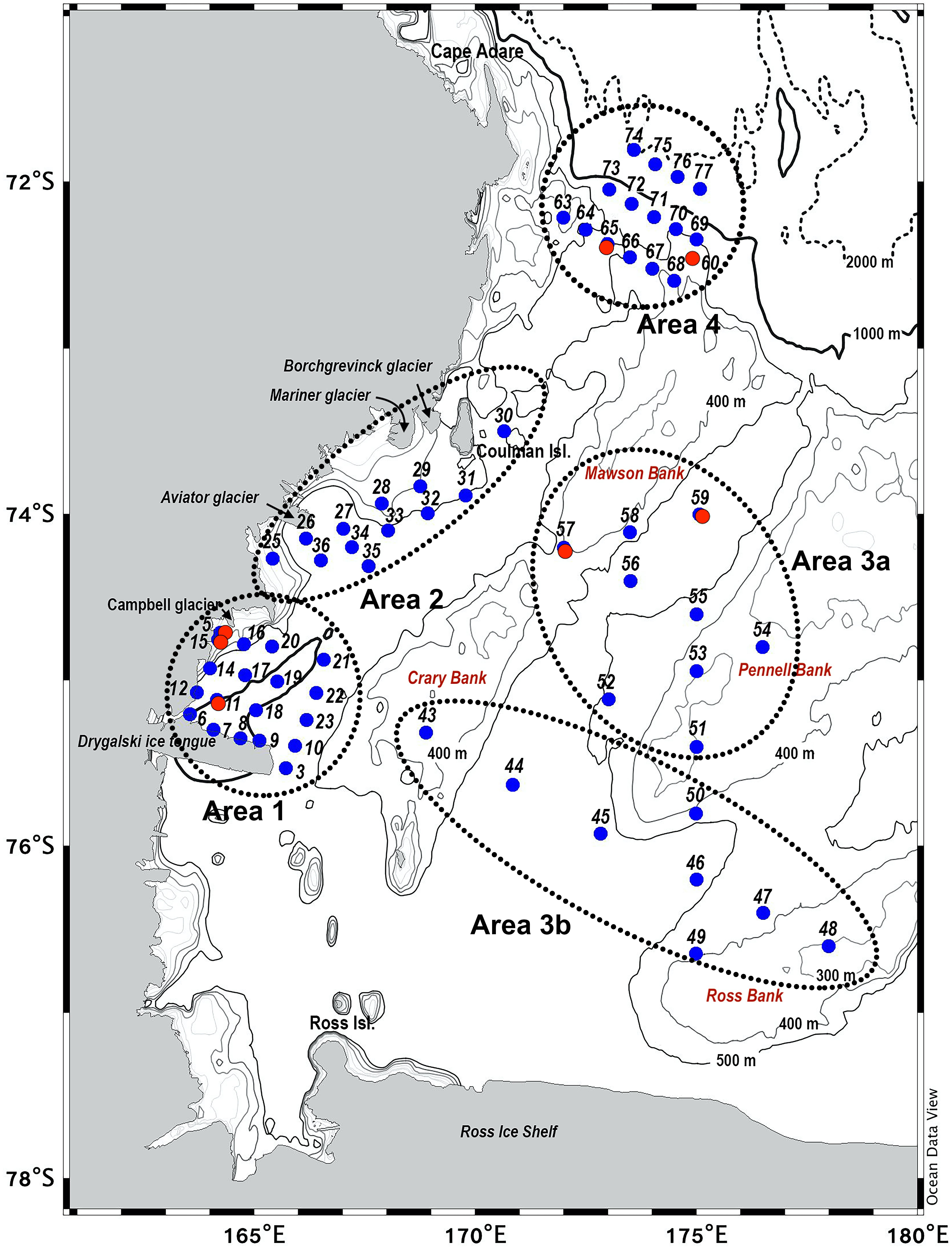
Figure 1. Stations sampled in P-ROSE and CELEBeR projects. Dotted lines indicate: Area 1, St. 3–23; Area 2, St. 25–36; Area 3a, St. 43–50; Area 3b, St. 51–59; Area 4, St. 63–77. Red points indicate repeated stations.
The maximum PSII photochemical efficiency (Fv/Fm) was determined on board using a Phyto PAM ED (Walz, Heinz Walz GmbH, Eichenring 6-91090 Effeltrich-Germany). All samples were acclimated in the dark for 30 min before analysis to minimize the non-photochemical dissipation of excitation, and measurements were blank corrected by filtering the sample through 0.2 μm filter (Cullen and Davis, 2003). For Fv/Fm analysis, samples were illuminated with a saturating pulse as reported in Maxwell and Johnson (2000), and values derived from the formula Fv/Fm = (Fm − F0)/Fm.
For the analysis of the total phytoplankton biomass and the micro, nano, and pico size fractions (> 20, 2-20, and < 2 μm, respectively), 500 mL of sea water were filtered on board through Whatman GF/F and Nuclepore membrane filters (25 mm diameter) and rapidly frozen at −80°C. Sample fractionation was performed following a protocol of serial filtration as reported by Mangoni et al. (2017). Frozen filters were processed in Italy for the determination of chl a and phaeopigments (phaeo) content, using a solution of 90% acetone according to Holm-Hansen et al. (1965), with a spectrofluorometer (Shimadzu, Mod.RF–6000; Shimadzu Corporation-Japan) checked daily with a chl a standard solution (Sigma-Aldrich). The pheao:chl a ratio was used as proxy of grazing activity on phytoplankton cells (Shuman and Lorenzen, 1975; Collos et al., 2005).
For the determination of phytoplankton functional groups by chemotaxonomic criteria (Mackey et al., 1996; Wright et al., 2010), 2 L of seawater were filtered on board onto Whatman GF/F filters (47 mm diameter) and stored at −80°C until pigments HPLC analysis were performed back in Italy. HPLC pigments separations were made on an Agilent 1100 HPLC (Agilent technologies, United States) according to the method outlined in Vidussi et al. (1996) as modified by Brunet and Mangoni (2010). The system was equipped with an HP 1050 photodiode array detector and a HP 1046A fluorescence detector for the determination of chlorophyll degradation products. Instrument calibration was carried out with external standard pigments provided by the International Agency for 14C determination-VKI Water Quality Institute. The relationship between spectrofluorimetric chl a and HPLC chl a for all samples was strong (p < 0.001, y = 1.28 ⋅ x + 0.26, R2 = 0.82, n = 198). Pigment concentrations were used to estimate the contributions of the main functional groups to the total chl a (Supplementary Table 2) using the matrix factorization program CHEMTAX 1.95.
For the determination of macronutrient concentrations, i.e., NO3–, NO2–, NH4+, Si(OH)4, PO43–, samples were taken directly from the Niskin bottles and stored at −20°C in 20 mL low-density polyethylene (LDPE) containers until laboratory analysis. The analyses were performed using a five-channel continuous flow autoanalyzer (Technicon Autoanalyser II, Systea S.p.A. Analytical Technologies, Italy), according to the method described by Hansen and Grasshoff (1983) adapted to current instrumentation. The accuracy and precision of the method were checked by Certified Reference Material (CRM) MOOS-3 (Seawater Certified Reference Material for Nutrients1). The measured nutrient concentrations in CRM were not significantly different from the certified values (p < 0.05).
For the analysis of total dissolved iron, seawater samples were filtered through 0.4 μm pore-size PC membranes, collected in 200 mL poly propylene bottles and stored at −20°C until analysis. At selected stations, seawater samples were collected by a 5 L Teflon-lined GO-FLO bottle (which was deployed on a kevlar 6 mm diameter line and closed using a polyvinyl chloride messenger) at ∼20 and ∼100 m depth. Seawater was transferred in acid-cleaned 2 L LDPE bottles and immediately treated as reported by Rivaro et al. (2019). Total dissolved iron was determined by ICP-MS after a metal pre-concentration procedure through co-precipitation with Mg(OH)2 based on a work by Wu and Boyle (1998) and Rivaro et al. (2019), with seawater transferred in acid-cleaned 2 L LDPE bottles and immediately treated as reported by the above mentioned authors.
Statistical Analysis
In order to investigate the relationship between inorganic nutrient concentrations (NO3, PO4, Si), salinity, temperature, upper mixed layer (UML), total phytoplankton biomass (chl a) and the percentage contribution of diatoms and haptophytes in different sub-systems, a principal component analysis (PCA) based on a Spearman’s correlation matrix was performed dealing missing data with pairwise deletion. For a synthetic interpretation of data, the UML value in the PCA was considered assigning the score 1 when the observations fall within the upper mixed layer, and the score 0 when the observations fall below the upper mixed layer. The analyses were made using XLSTAT-Ecology 2019 software, and results are presented using diagrams of factor loadings (projection of the variables on the factor-plane described by the 1st and 2nd principal factors) in a correlation circle chart. In Supplementary Table 3 are reported Spearman’s correlation matrix with values in bold different to 0 with a significant level alpha (p = 0.95).
Results
To better define physical, chemical, and biological features, sampling areas (Figure 1 and Supplementary Table 1) will be discussed separately in the following subsections. Additionally, repeated stations will be considered in a separate subsection to highlight their temporal variability (Figures 1, 10, 11). The principal abbreviation used in the text are reported in Table 1.

Table 1. Abbreviations used in the text.
Area 1 (January 9–15, 2017)
Area 1 includes stations located in Terra Nova Bay (TNB) within an area extending from Cape Washington to the northern shores of the Drygalski Ice Tongue (DIT) a littoral feature that must be considered when evaluating the forcing factors influencing the structural and functional characters of phytoplankton communities. UML depth (Supplementary Table 1) was not homogeneous, varying from 9 to 57 m, and was particularly shallow near DIT, especially at the tongue’s edge (station 3) where it was ∼1 m. UML deepens north-westward reaching its maximum at stations 14 and 15, close to the coast. These stations were also characterized by the highest surface temperature measured in TNB and in all areas considered in this study. At the DIT edge, stations presented the lowest salinity observed in TNB. Θ/S diagrams (Figures 2A–E) highlight significant temperature and salinity differences in the surface layer among areas. Moreover, the TNB Θ/S diagram showed the typical summer vertical structure of this area, with the Dense Shelf Water (DSW) at the bottom and the lightest Antarctic Surface water (AASW) occupying the top 100 m layer.
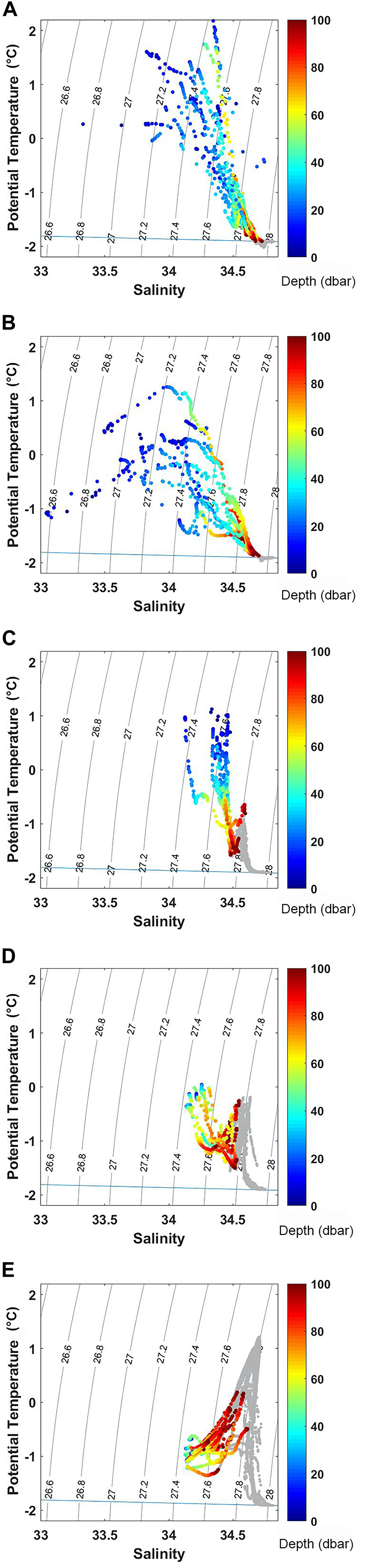
Figure 2. Θ/S diagram for each sub-system: Area 1 (A), Area 2 (B), Area 3a (C), Area 3b (D), Area 4 (E). The color bar indicates the first 100 m depth, deeper layers are reported in gray.
Considering the distribution of integrated chl a for the 0–100 m layer, high biomass levels were reported particularly near the coastline, with a maximum of 271.81 mg chl a m–2 at station 14 (Figure 3). Furthermore, there was an evident eastward decreasing concentration gradient except for station 3, in proximity of DIT, with a relative maximum of 174.42 mg chl a m–2. The mean vertical profile of chl a (Figures 4A–E), showed a linear decrease toward the bottom with values ranging from ∼2.15 to 0.32 μg L–1 (at 0 and 100 m, respectively). In the first 20 m, mean values always exceeded 2 μg L–1, and the highest values in the first 0–40 m was found at coastal station 14, with the maximum of 4.59 μg L–1. Mean chl a and phaeo:chl a ratio (Figures 5A–E) in Area 1 were 1.45 μg L–1 and 0.87, respectively. The percentage contribution of the main functional groups to the total biomass (Figures 6A–E) showed diatoms as the dominant group with a mean of 67%, followed by haptophytes with 26%, and among other minor groups, chlorophytes reached 3% and the rest were almost absent. Regarding the community size structure (Figures 7A–E), micro- and nano-phytoplankton both showed a percentage of 39%, and pico-phytoplankton accounted for 22%. Photosynthetic maximum quantum efficiency (Figures 8A–E) (Fv/Fm) was 0.33 for the entire area, with values greater than 0.4 within and below UML and the maximum of 0.58 in surface waters at coastal station 5.
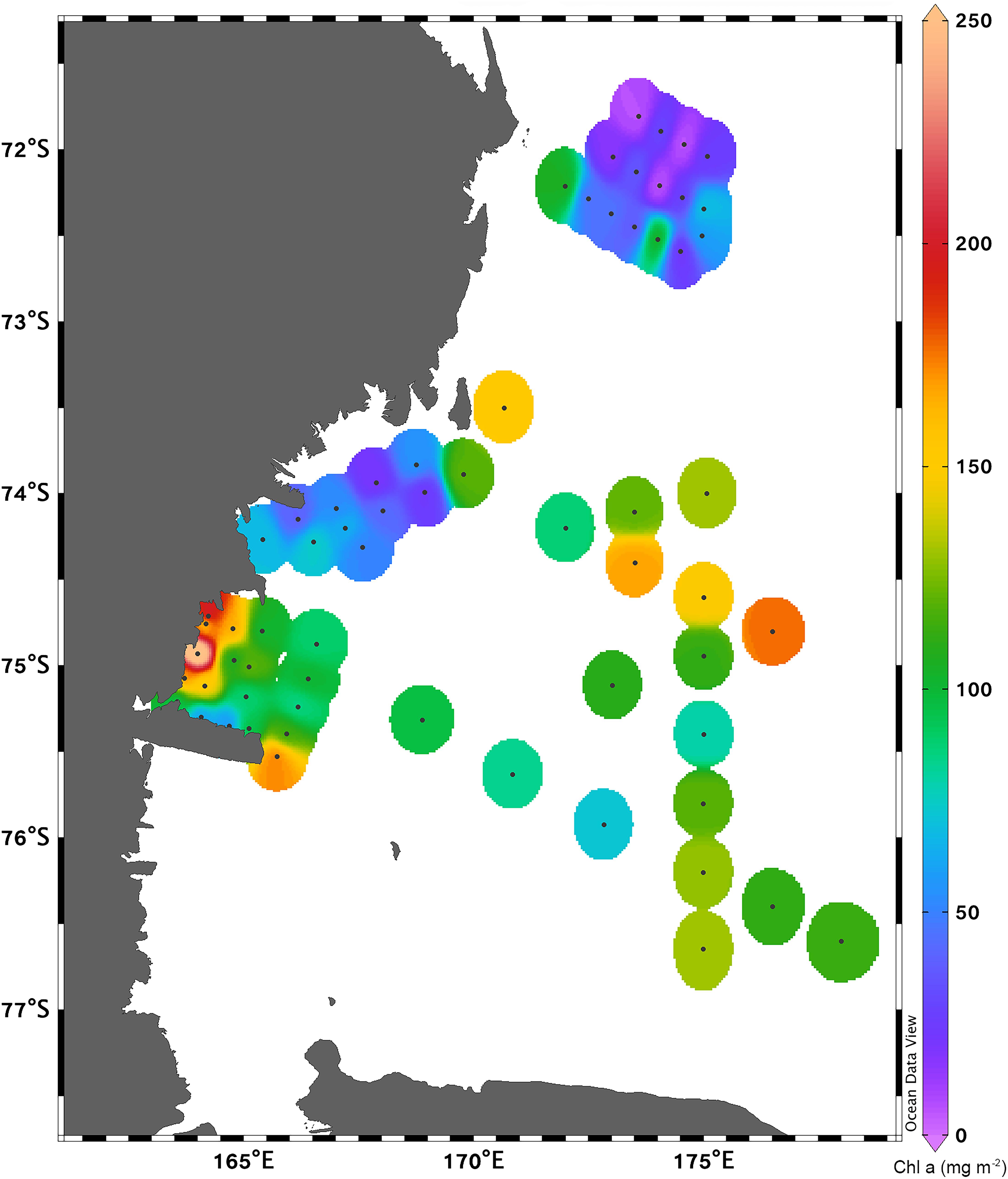
Figure 3. Spatial distribution of integrated phytoplankton biomass (mg chl a m– 2) in the 0—100 m layer.
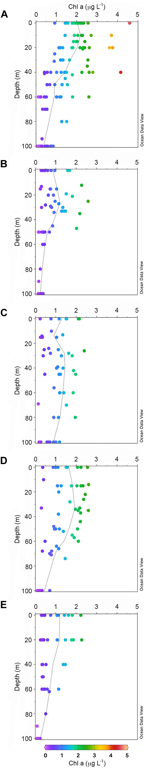
Figure 4. Mean vertical profiles and scatter plot of chl a (mg L–1) for each sub-system: Area 1 (A), Area 2 (B), Area 3a (C), Area 3b (D), Area 4 (E). The black line indicates the mean chl a concentration of the entire area.
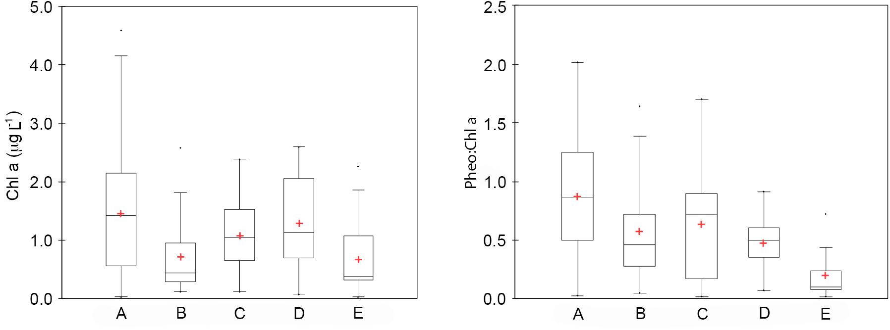
Figure 5. Boxplots of chl a (mg L–1) and phaeo:chl a ratio for each sub-system: Area 1 (A), Area 2 (B), Area 3a (C), Area 3b (D), Area 4 (E). The black line is the median and the red cross is the mean.
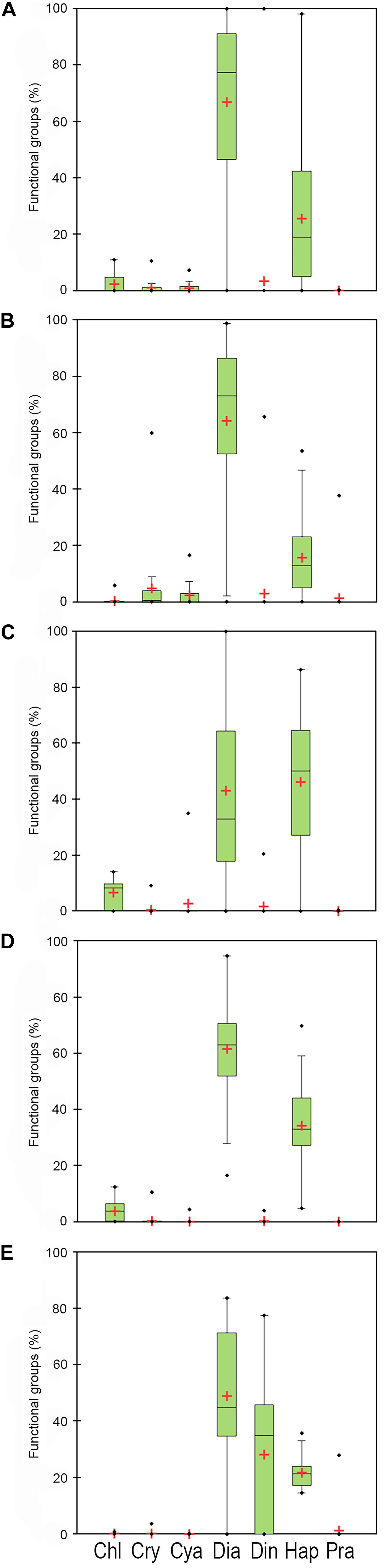
Figure 6. Percentage contribution of the main functional groups to total biomass; i.e., chlorophytes (Chl), cryophytes (Cry), cyanophytes (Cya), diatoms (Dia), dinoflagellates (Din), haptophytes (Hap), prasinophytes (Pra), in Area 1 (A), 2 (B), 3a (C), 3b (D), and 4 (E). The black line is the median and the red cross is the mean.
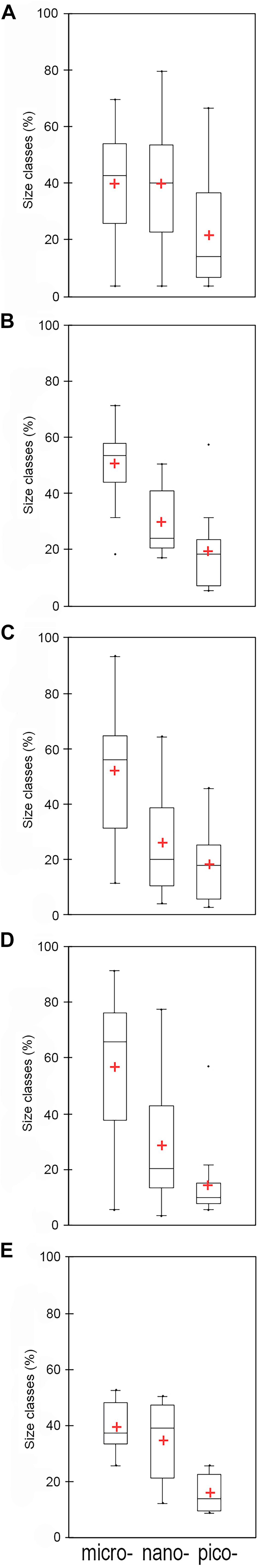
Figure 7. Percentage contribution of size classes, i.e., micro- (> 20 μm), nano- (20–2 μm), pico- (< 2 μm), in Area 1 (A), 2 (B), 3a (C), 3b (D), and 4 (E). The black line is the median and the red cross is the mean.
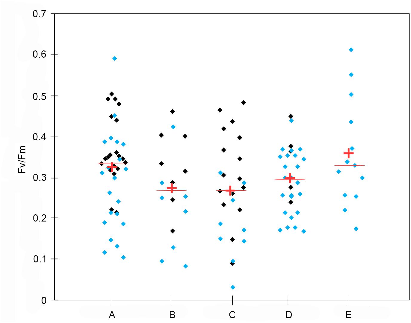
Figure 8. Scattergram of photosynthetic maximum quantum efficiency (Fv/Fm) for different sub-systems: Area 1 (A), 2 (B), 3a (C), 3b (D), and 4 (E). Light blue dots indicate samples within UML, and black dots indicate samples below UML. The line is the median and the cross is the mean.
Regarding the vertical distribution of inorganic nutrients (data not shown) DIN varied from 9.1 to 20.0 μmol L–1 in the upper 20 m; below this layer, DIN exceeded 27.0 μmol L–1. PO43– ranged from 0.45 to 1.69 μmol L–1 in UML, reaching concentrations up to 2.29 μmol L–1 below UML. Si(OH)4 ranged from 23 to 63 μmol L–1 in UML, increasing to 79 μmol L–1 below UML. The mean value of dissolved iron concentration in the entire area at ∼30 m was 0.90 ± 0.37 nM.
PCA analyses (Figures 9A–E) explained 76.33% of the total variance, with F1 and F2 axis representing 64.65 and 11.68% of total variance, respectively. UML and temperature overlapped with positive F1, and chl a and diatoms displayed a high correlation factor with F1 (0.77 and 0.8, respectively). Haptophytes, salinity, DIN, and PO43– presented similar (negative) correlation factors with F1, and haptophytes were inversely correlated with diatoms. Si(OH)4 was the only variable highly (0.9) correlated with F2.
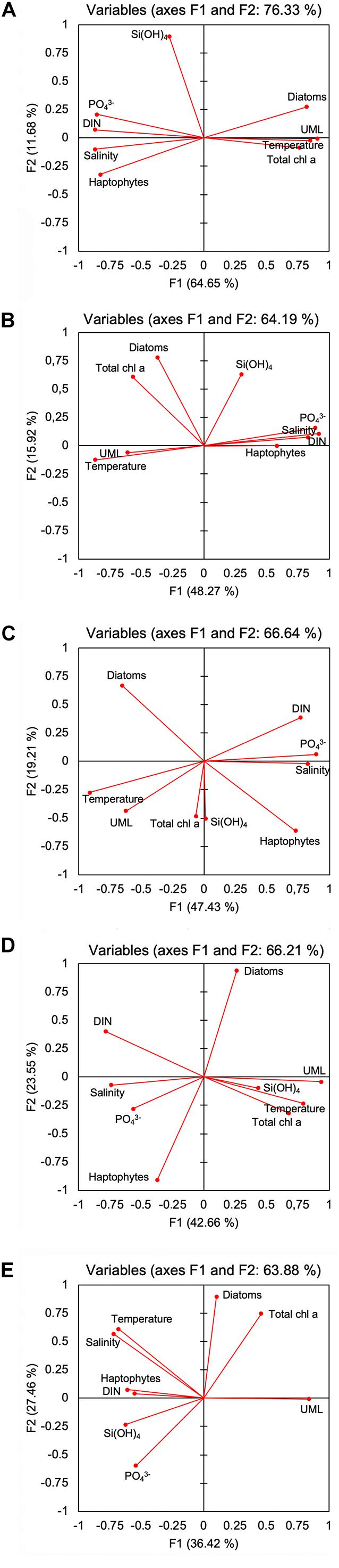
Figure 9. Correlation plot from Principal Component Analysis (PCA) on axes F1 and F2, with projection of variables biological (chl a; percentage contribution of diatoms and haptophytes to total biomass) and environmental variables (salinity; temperature; dissolved inorganic nitrogen, NO2 + NO3–, silicate, Si(OH)4; phosphate, PO43–; upper mixed layer, UML) for Area 1 (A), 2 (B), 3a (C), 3b (D), and 4 (E) in the factors space.
Area 2 (January 12–22, 2017)
Area 2 was surveyed by a cruise track stretching from the Aviator ice tongue to Coulman Island (Figure 1). This sub-system was characterized by a shallow UML (Supplementary Table 1) especially at stations 25, 26, 27 near the edge of Aviator ice tongue (UML < 1 m), and the deepest UML depth (32 m) was observed at station 30 situated east of Coulman Island. Stations near Aviator ice tongue were characterized by the intrusion of relatively warm water (salinity ∼34) into the subsurface layer. Station 30 was characterized by the coldest (−1.21°C) and densest surface layer in this region, indicating that its physical characteristics were completely different from those of other stations in the area. Moreover, Θ/S diagrams (Figures 2A–E) evidenced that this area was characterized by the lowest surface salinity. The integrated chl a in the first 100 m was 20.92-69.40 mg chl a m–2 except at stations 30 and 31, where values reached 152.40 and 119.56 mg chl a m–2, respectively (Figure 3). In the entire Area 2, a slight decreasing concentration gradient was observed from coastal stations to those located northward. Mean chl a values (Figures 4A–E) exceeded 1 μg L–1 between 10 and 25 m, and were lower than 0.6 μg L–1 below this depth, reaching a minimum of 0.24 μg L–1 at 100 m. The points exceeding 2.58 μg L–1 in the first 30 m belonged to station 31. Mean chl a concentration and phaeo:chl a ratio for the entire area were 0.72 μg L–1 and 0.57, respectively (Figures 5A–E). The percentage contribution of the main functional groups to the total biomass (Figures 6A–E), showed a dominance of diatoms with 64%, while haptophytes accounted for 16% of the total biomass. Other groups were nearly absent, except cryptophytes (4.7%), and cyanophytes (2.3%). Regarding the community size structure, biomass was mainly dominated by micro-phytoplankton (51%), while nano- and pico-phytoplankton represented 30 and 19%, respectively (Figures 7A–E). Photosynthetic maximum quantum efficiency (Figures 8A–E) was represented by a mean Fv/Fm value of 0.27 for the entire area, and a maximum of 0.46 at station 30 (0 m), being over 0.4 only at stations 30 and 31.
DIN concentration increased from the surface to deeper waters (12.94–24.35 μmol L–1) except at station 30, where it was more homogeneously distributed along the water column ranging between 25 and 30 μmol L–1. PO43– reached 0.82–1.64 μmol L–1 at the surface and increased up to 2.08 μmol L–1 at deeper levels, displaying a similar trend to that of DIN. Si(OH)4 concentration was 33–58 μmol L–1 within UML, and rapidly increased below this layer, reaching 80 μmol L–1. Mean dissolved iron concentration was 1.02 ± 0.40 nM at ∼30 m.
PCA (Figures 9A–E) explained 64.19% of the total variance, with the F1 and F2 axis accounting for 48.27 and 15.92% of the total variance, respectively. PCA highlighted a strong correlation between temperature and UML, both inversely correlated with DIN, salinity, haptophytes, and PO43–. Chl a and diatoms, in the fourth quadrant of the PCA biplot, had similar correlation factors with F1 and F2. Si(OH)4 placed in the first PCA quadrant, showed a similar factor of correlation with F2 to that of chl a and diatoms.
Area 3
Stations of this area were distributed on a track along 175°E within a large area of the south-central Ross Sea, representing an off-shore system divided by us into two sub-systems (Areas 3a and 3b), which we discussed separately owing to the different sampling time imposed by adverse meteorological conditions. Areas 3a and 3b include stations 43–50 and 51–59, respectively.
Area 3a (January 26–27, 2017)
The UML depth (Supplementary Table 1) highlights the presence of a shallow mixed layer < 25 m excluding station 50, where UML was 32 m. Stations located between Crary and Pennell banks were characterized by a shallow UML, with depth of 7 and 1 m (station 44 and 46, respectively). The Θ/S diagram (Figures 2A–E) characterized this area by a vertically quasi-homogeneous salinity in the top 100 m at all stations, except for the easternmost station (43), where a fresher and more stratified surface layer was observed.
The distribution of integrated chl a in the first 100 m ranged from 132.13 to 71.74 mg chl a m–2 (station 49 and 45, respectively), with relatively higher values moving south-eastward (Figure 3). Chl a distribution was rather homogeneous in the first 70 m (Figures 4A–E), with the mean vertical profile showing values of ∼1.2 μg L–1, except at 10 m (0.8 μg L–1). The highest phytoplankton biomass recorded in this area was 2.39 μg L–1 chl a at 26 m, while the mean total biomass and phaeo:chl a ratio in the entire area were 0.8 μg L–1 chl a and 0.63, respectively (Figures 5A–E). Haptophytes and diatoms displayed similar percentage, representing 46 and 43% of the phytoplankton community, respectively (Figures 6A–E), while chlorophytes and cyanophytes accounted for 6 and 2.5% of total biomass, respectively. Regarding size structure, micro-phytoplankton dominated the community with a mean of 57%, while nano- and pico-phytoplankton represented instead 29 and 15% of phytoplankton biomass, respectively (Figures 7A–E). The maximum quantum yield (Figures 8A–E), showed a mean of 0.27, with low values below UML and high values at deeper layers.
DIN vertical distribution ranged between 21.58 and 26.67 μmol L–1 in the first 50 m, and increased to 32.07 μmol L–1 at 100 m. PO43– in the 0–50 m layer ranged from 1.10 to 2.01 μmol L–1, and reached 2.47 μmol L–1 at deeper levels. The mean dissolved iron concentration at ∼30 m was 0.73 ± 0.40 nM.
PCA (Figures 9A–E) explained 66.64% of variance, with the F1 and F2 axis accounting for 47.43 and 19.21% of total variance, respectively. Chl a and Si(OH)4 almost overlapped with negative axis F2 (factor loading of −0.043 and −0.503, respectively). Haptophytes, UML, and temperature correlated in a similar manner with F2 and differently with F1. In particular, haptophytes, salinity, PO43–, and DIN showed the same correlation with F1, and were inversely correlated with diatoms. Temperature, UML, and diatoms were negatively correlated with F1 (−0.91, −0.63, −0.66, respectively).
Area 3b (January 29-30, 2017)
In Area 3b the weather condition led to a deepening of UML compared to that of Area 3a, with depths ranging between 38 and 69 m and a mean depth of 56 m (Supplementary Table 1). The presence of a deeper UML was also highlighted by the Θ/S diagram (Figures 2A–E), with the salinity and potential temperature values of the first 50 m concentrated in a small region of the Θ/S diagram. Figures 2A–E also showed the influence of the modified Circumpolar Deep Water in this area on the lower part of the top 100 m layer, as shown by the potential temperature increase from 80 to 100 m depth.
The integrated chl a ranged from 176.59 to 79.39 mg chl a m–2 (station 54 and 51, respectively), with the presence of an increasing gradient of concentrations moving from stations in the north-western part to those in the south-east (Figure 3). The integrated value of chl a concentration at station 54 was the highest observed in the south-central Ross Sea during this cruise. The vertical distribution of chl a (Figures 4A–E) showed higher levels of biomass in the first 50 m than in lower levels, with values up to 2.55 μg L–1 (14 m), and a mean profile that exceed 1.77 μg L–1 in the 10–40 m layer. Below 50 m, chl a decreased to 0.20 μg L–1 at 100 m. The mean total chl a and phaeo:chl a ratio for this area were 1.30 μg L–1 and 0.47, respectively (Figures 5A–E). Diatoms represented 62% of the community, and haptophytes represented 36% (Figures 6A–E). Among minor groups, chlorophytes reached 3.5%. Approximately 51% of the phytoplankton community was represented by micro-phytoplankton, while nano- and pico-phytoplankton represented 30 and 19%, respectively (Figures 7A–E). The mean Fv/Fm was 0.30, with single values reaching 0.45 within and below UML (Figures 8A–E) and a minimum of 0.17 at 0 m (station 57).
DIN concentrations ranged between 15.04 and 22.63 μmol L–1 in the first 50 m, while at deeper levels they increased up to 31.56 μmol L–1. PO43– displayed the same pattern of distribution as DIN, ranging from 0.86 to 1.97 μmol L–1 in the first 50 m, and increasing up to 2.5 μmol L–1 at 100 m. Regarding dissolved iron concentration, the mean value observed in this area at ∼30 m was 1.07 ± 0.40 nM.
PCA (Figures 9A–E) explained 66.21% of the variance, with axes F1 and F2 accounting for 42.66 and 23.55% of total variance, respectively. The distribution of active variables highlights the inverse correlation between diatoms and haptophytes. Chl a, temperature, UML and to a lesser extent, also Si(OH)4, showed a similar correlation with F1. Salinity was inversely correlated with UML, showing a negative correlation with F1 similar to that of DIN (−0.78 and −0.74, respectively), while PO43– and haptophytes presented correlation factors of −0.57 and −0.37.
Area 4 (February 6–8, 2017)
Area 4 represents the northernmost sampled area of the cruise, with stations distributed along three short transects at the interface with the open Southern Ocean waters. In this area, UML depth (Supplementary Table 1) showed a pronounced variability, with high values in the transect registered over the shelf. Here the mean UML depth was 82 m and reached the maximum of 133 m at station 78, in the center of the Drygalski Through. The shallowest UML at the transect was observed close to the shelf break and was characterized by a mean value of 48 m ranging from 45 to 58 m. UML depth over the continental slope, was 67 m on average, with the maximum of 90 m measured at the westernmost station. Θ/S diagram in this region (Figures 2A–E) showed cold and fresh AASW in UML, and warm and salty Circumpolar Deep Water (CDW) in the layer below it.
The integrated chl a concentration in the first 100 m ranged from 106.80 to 6.63 mg chl a m–2 at station 63 and 74, respectively (Figure 3). Biomass levels in the southern zone of the area were relatively higher than those in the northern zone. The distribution of chl a slightly decreased from the surface, with a recorded a maximum of 2.27 μg L–1 at 20 m and a mean maximum of 0.83 μg L–1, to the deeper layer, with a recorded mean value of 0.22 μg L–1 (Figures 4A–E). Total biomass and the phaeo:chl a ratios in this area are reported in Figure 5. Mean chl a and phaeo:chl a ratio were 0.68 μg L–1 and 0.20, respectively, representing the lowest values among areas in this study. Diatoms were the most abundant group (53%), while dinoflagellates and haptophytes showed percentage of 24 and 23%, respectively (Figures 6A–E). Micro- and nano-phytoplankton represented 43 and 37% of biomass, respectively, while pico-phytoplankton accounted only for 20% (Figures 7A–E). Regarding photosynthetic maximum quantum efficiency (Figures 8A–E), the mean Fv/Fm value in the area was 0.36, and all data fell within UML owing to the width of this layer.
DIN ranged between 21.5 and 27.0 μmol L–1 except at station 65, where its concentration increased up to 31.8 μmol L–1. PO43– showed a distribution analogous to that of DIN, both in terms of extent of variation and depth profile. Si(OH)4 ranged between 51 and 69 μmol L–1 within UML, while below UML, it increased to 100 μmol L–1. The mean dissolved iron concentration was 0.67 ± 0.33 nM.
PCA analysis explained 63.88% of the variance, with axes F1 and F2 accounting for 36.42 and 27.36% of total variance, respectively (Figures 9A–E). Chl a and diatoms showed a similar correlation with F2 (0.75 and 0.98, respectively), and chl a was inversely correlated with PO43–. UML overlapped with axis F1, and was inversely correlated with haptophytes and DIN. Temperature and salinity were strongly correlated (fourth quadrant), showing correlation factors similar to those of Si(OH)4, PO43–, DIN, and haptophytes with axis F2.
Repeated Stations
Area 1: Stations 5 (January 10 and 22), 11 (January 13 and February 11) and 15 (January 14, 23 an February 11)
At station 5, which corresponds to “Mooring L,” chl a concentration was ∼2.20 μg L–1 in the 0–20 m layer on January 10 (Figure 10). Below this depth, values decreased to 1.27 μg L–1 (50 m) reaching a minimum of 0.77 μg L–1 at 100 m. On January 22, chl a showed a general decrease, ranging from 1.20 to 0.28 μg L–1 (at 15 and 100 m, respectively), with a distribution pattern similar to that observed during the first sampling. Diatoms represented more than 90% of biomass in the 0–20 m layer on January 10, while haptophytes reached a relative high percentage (57%) below 50 m. In the second sampling, diatoms still dominated the community, although haptophytes were distributed more homogeneously in the water column than those in the first sampling. The ratio phaeo:chl a in the first sampling ranged from 0.6 to 1 (at 0 and 100 m, respectively), while on January 22, values ranged from 0.9 to 2 below 15 m, and were 0.7 in the surface layer. Surface temperature reached 2.33°C on January 10, and a thermocline was present below 15 m with values that decreased down to −0.92°C at 35 m. Below this depth, temperature slightly decreased to −1.67°C at 100 m. After 12 days, temperature displayed a general decrease ranging from 1.20 to −1.85°C, although the distribution pattern was similar to that observed in the first sampling. Salinity distribution on January 10 was almost homogeneous in the entire water column, with values that slightly increased from the surface to the bottom. After 12 days, salinity significantly decreased in the first 18 m ranging from 34.34 to 34.36 (at 0 and 18 m, respectively). Below 18 m, the vertical profile was similar to that observed before (Figure 10).
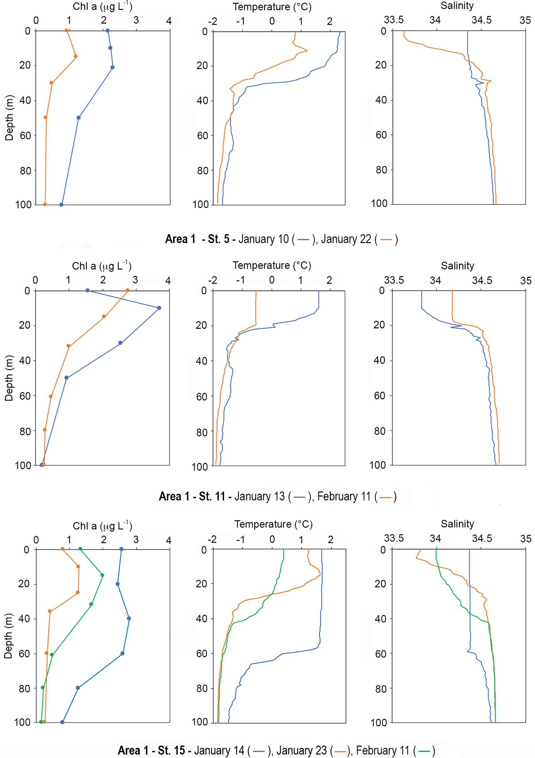
Figure 10. Vertical profiles of chl a (μg L–1), temperature, and salinity at resampled stations in Area 1. Stations 5, 11, 15.
At station 11, representing Mooring D near DIT, on January 13, chl a was the highest in the first 30 m of the water column, with a maximum of 3.70 μg L–1 at 10 m and values < 1 μg L–1 below 30 m (Figure 10). On February 11, biomass was still higher in the first 15 m than below that depth, ranging from 2.76 to 2.06 μg L–1 (at 0 and 15 m, respectively). During the first sampling, diatoms represented more than 90% of the community in the first 30 m and haptophytes reached 55% below this layer. On February 11, diatoms strongly dominated (80%) in the entire water column, both with high and low biomass levels, and haptophytes represented ∼20% of the community. The phaeo:chl a ratios were always close to 0.5 in the entire water column in both sampling periods. Water temperature on January 13 was ∼1.41°C in the first 10 m and showed positive values until 20 m. Below 30 m, values ranged between −1.20 and −1.80°C. During the second sampling, temperature was always below 0, and the first 20 m were characterized by values of −0.54°C that decreased to −1.80°C at 100 m. Salinity showed a similar pattern between January 13 and February 11, with homogeneous values in the first 10 m lower than those in deeper layers, which showed a significant salinity increase during the second sampling (Figure 10).
Station 15 is an LTER station (MOA-TNB LTER_EU_IT_17-005-M) in TNB, indicated with name Santa Maria Novella (SMN), sampled three time during the cruise (Figure 10). On January 14, chl a was distributed rather homogeneously in the first 60 m with a mean of 2.55 μg L–1. On January 23, a net decrease was observed in the 0–40 m layer (mean of 1.11 μg L–1) with concentrations ∼ 0.34 μg L–1 from 40 to 100 m. On February 2, a second bloom was observed with concentration increasing in the first 60 m, reaching a subsurface maximum of 2 μg L–1 at 15 m, and slightly decreasing from this depth to 0.25μg L–1 at 100 m. The phaeo:chl a ratio in the first sampling ranged between 0.5 and 0.8 (at 0 and 80 m, respectively), reaching the maximum of 1.2 at 100 m. During the second sampling, ratios were low until 25 m (∼0.5), and exceeded 1 below this depth. On February 2, values were ∼0.5 until 30 m depth, increasing below that depth and reaching 1.7. Regarding phytoplankton functional groups, diatoms strongly dominated on January 14 especially in the first 60 m, while haptophytes increased below this depth to up to 43%. During the second sampling, diatoms dominated in the first 40 m, while haptophytes increased below this depth and became dominant group with percentages exceeding 50%. On February 2, diatoms dominated homogeneously in the entire water column ranging from 66 to 87%, while haptophytes represented the second most abundant group showing a complementary pattern of distribution to that of diatoms. Regarding temperature, the water column displayed homogeneous values in the first 60 m (∼1.65°C) during the first sampling, with a net thermocline between 58 and 65 m. On January 23, a significant temperature decrease was observed below 30 m, with a shallower thermocline between 18 and 30 m, and values that slightly increased from the surface to 15 m. On February 2, temperature further decreased in the first 30 m ranging from 0.38 to −0.84°C (at 0 and 40 m, respectively). Below this depth, temperature was similar to that observed on January 23. The vertical salinity profile on January 14 was characterized by values ∼ 34.37 in the first 60 m, reaching 34.61 at 100 m. On January 23, salinity ranged from 33.82 to 34.55 (at 0 and 30 m, respectively), and slightly increased below this depth to 34.66 at 100 m. On February 2, the water column showed a different profile, with values increasing in the first 40 m (from 33.99 to 34.45) and displaying a similar profile to that observed on January 23 below 40 m (Figure 10).
Area 3b: Stations 59 (January 17 and 30) and 57 (January 30 and February 9)
Station 59, in the north-central Ross Sea as part of Joides Basin, represents the Mooring B site (LTER_EU_IT_17-002-M). On January 17, Chl a ranged between 2.49 and 2.45 μg L–1 in the first 20 m, and from 1.79 to 1.22 μg L–1 between 40 and 100 m (Figure 11). On January 30, biomass decreased especially in the surface layer, varying from 1.56 to 1.961 μg L–1 (at 0 and 34 m, respectively) and reaching 0.195 μg L–1 at 100 m. Regarding the phaeo:chl a ratio, values were 0.4 on January 17 at all depths, except at 100 m (1.5). During the second sampling, ratios were 0.3 in the first 55 m, ranging between 0.7 and 0.8 below this depth. Diatoms and haptophytes coexisted with similar percentage throughout the water column during the first sampling, with a slight prevalence of haptophytes at 100 m. On January 30, diatoms were the dominant group with percentages up to 73%, with haptophytes distributed homogeneously along the water column as the second most abundant group. Regarding temperature, the vertical distribution displayed a wide homeothermic profile in both samplings, although values increased on January 30 (∼0.3°C increase) and the weak thermocline sunk from 50 to 60 m. Below this depth values increased toward the bottom on January 17, while this trend was less evident on January 30. Regarding salinity, vertical profiles were similar in both samplings, with the first ∼50 m characterized by homogeneous values that increased toward the bottom below this depth (Figure 11).
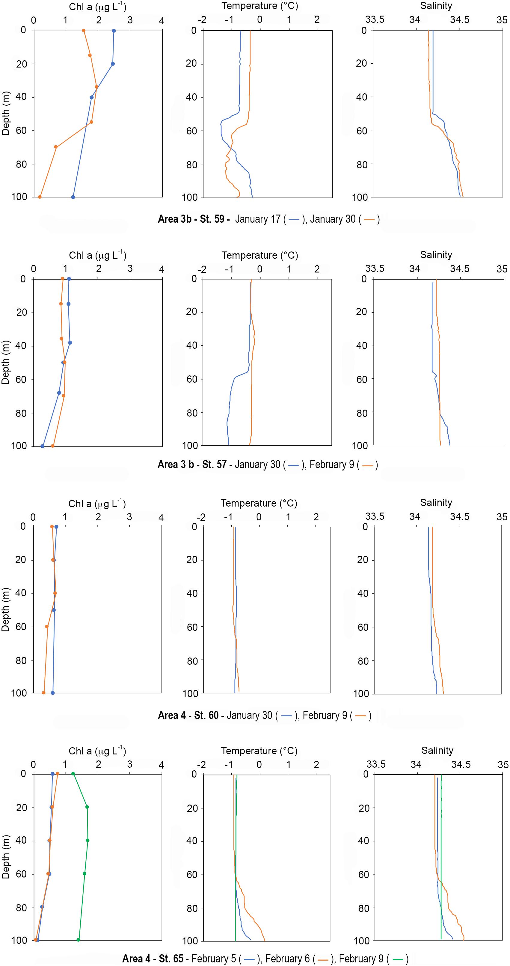
Figure 11. Vertical profiles of chl a (μg L–1), temperature, and salinity at resampled stations in Area 3b, stations 57 and 59, and in Area 4, stations 60 and 65.
Station 57 was located between Mawson Bank and Crary Bank (Figure 1). Vertical profiles of chl a were similar on January 30 and February 9, with values ranging between 1.13 and 0.9 μg L–1 in the 0–50 m layer with a net dominance of diatoms. Below 50 m, diatoms still dominated the community and chl a decreased to 0.28 and 0.603 μg L–1 on January 30 and February 9, respectively. Regarding the phaeo:chl a ratio, values ranged between 0.39 and 0.67 in the first 50 m on January 9, and exceeded 1 below 69 m, while ratios were lower than 0.5 in the first 50 m on February 9, increasing up to 0.89 at 100 m. Temperature did not vary much between sampling times, ranging between −0.33 and −0.39 in the first 50 m. Below this depth, on January 30 temperature decreased to −1.09°C, with a weak thermocline near 58 m, while values on February 9 were similar to those observed at the surface. The distribution of salinity was nearly homogeneous in the water column on both sampling times, being ∼34.17 and ∼34.22 on January 30 and February 9, respectively (Figure 11).
Area 4: Stations 60 (January 30 and February 9) and 65 (February 5, 6 and 9)
At station 60, on January 30 and February 9 the distribution of chl a was homogeneous in the entire water column, and values ranged from ∼0.73 to ∼0.61 μg L–1 at 0 and 100 m (Figure 11), respectively. The phaeo:chl a ratio was 0.3 in the entire water column both sampling times. The phytoplankton community was dominated by diatoms, exceeding 60%, while haptophytes and dinoflagellates represented 20 and 18%, respectively. Temperature and salinity were homogeneous in the entire water column, with values around −0.85°C and 34.18, respectively (Figure 11).
Station 65 represents the Mooring G site. The distribution of chl a was similar between February 5 and February 6, ranging from ∼0.58 to 0.49 μg L–1 in the first 60 m, showing values close to 0.20 μg L–1 between 80 and 100 m (Figure 11). On February 9, a net increase of chl a was observed in the entire water column, and values ranged from 1.245 to 1.69 μg L–1 (at 0 and 40 m, respectively) reaching 1.41 μg L–1 at 100 m. Despite this increase, the phaeo:chl a ratio (0.5) was similar to that of previous samplings. On February 5, diatoms were dominant, and dinoflagellates represented the second most abundant group (close to 30%). Haptophytes represented between 15 and 35% of community. On February 6, group distribution did show much variation, although dinoflagellates became dominant at 100 m, representing 55% of biomass. On February 9, diatoms dominated with percentages between 61 and 82%, while dinoflagellates were the second most abundant group only at 0 m (22%). Below the surface, haptophytes reached 16–20% and dinoflagellates less than 10%. Regarding salinity and temperature distribution, both were distributed rather homogeneously in the first 60 m of the water column in the first two samplings, with values of ∼34.24 and −0.85°C, respectively. Below this depth, temperature increased up to −0.33 and 0.18°C at 100 m on February 5 and 6, respectively, while on February 9 temperature was −0.85 in the entire water column. Salinity increased to 34.42 and 34.54 at 100 m on February 5 and 6, respectively, while it remained 34.28 in the entire water column on February 9 (Figure 11).
Discussion
This study has confirmed some fundamental points on which the present paradigm about the role of the primary component in structuring the Ross Sea food web is based at different spatial and temporal scales. Phytoplankton community dynamics in the Ross Sea have been well documented in the past two decades, with massive blooms of haptophytes (P. antarctica) and diatoms showing different temporal and spatial pattern (DiTullio and Smith, 1996; Arrigo et al., 1999; Smith et al., 2014) and influencing the trophodynamics of the Ross Sea in different ways (DiTullio et al., 2000; Schoemann et al., 2005; Peloquin and Smith, 2007). In fact, diatoms are grazed at significant rates by zooplankton, such as copepods and krill, representing a crucial ecological link between primary production and higher trophic levels, while P. antarctica shows a different fate. This species can exist as a solitary cell, preyed by heterotrophic microplankton, or as mucilaginous colonies that mostly sink to the bottom largely without being grazed upon, except by some pteropods (Caron et al., 2000; DiTullio et al., 2000; Lonsdale et al., 2000; Dennett et al., 2001; Smith et al., 2003; Tagliabue and Arrigo, 2003; Tang et al., 2008; Elliott et al., 2009). Other functional groups are poorly represented, such as dinoflagellates, cryptophytes, cyanophytes, and chlorophytes, and are considered to have a minor role in the Antarctic food web (Andreoli et al., 1995; Arrigo et al., 2000; Smith et al., 2014; Mangoni et al., 2017; Phan-Tan et al., 2018). Nevertheless, we need to consider that a large part of the biological and physical information on the Ross Sea derive from studies performed in polynya areas or tracks repeated over the year to study the inter-annual variability of the system (DiTullio and Smith, 1996; Smith et al., 1996, Smith et al., 2006, 2010; Smith and Gordon, 1997; Saggiomo et al., 1998, 2002; Arrigo et al., 2000; DiTullio et al., 2000; Peloquin and Smith, 2007). In recent years, studies on the timing of productivity, distribution of main functional groups, as well as responses of key species to different environmental conditions have generated new questions on the drivers regulating primary production processes in the Ross Sea (e.g., Montes-Hugo and Yuan, 2012; Deppeler and Davidson, 2017; Mangoni et al., 2018, 2019; Park et al., 2019). Data obtained in this study during the summer 2017, clearly reveal that the Ross Sea is made up by a complex mosaic of sub-systems with physical, chemical, and biological features that change at different temporal and spatial scales.
Areas 1 (TNB) and 2, although neighboring coastal systems, presented different biological, chemical, and physical properties. In TNB, the mean integrated value of chl a was 127 ± 54 mg chl a m–2, while that of Area 2 was significantly lower (64 ± 38 mg chl a m–2), with only stations located near Coulman Island displaying similar concentrations to those of TNB (120 and 152 mg chl a m–2). The mean UML depth in TNB was 23 ± 13 m, being extremely shallow (1 m) at station 3 near DIT. Area 2 presented a shallower UML, with a mean depth of 12 ± 8 m, and values of ∼1 m at stations located in the inner part of the area (stations 25, 26, and 27). The slope of the nitrite plus nitrate plotted against phosphate [(NO3 + NO2):PO4] varied between areas, being 13.08 (R2 = 0.886) in TNB, and 14.37 in Area 2 (R2 = 0.179) (Figure 12). A previous study performed by Saggiomo et al. (2002) in TNB reported y = 11 in presence of diatom dominance during the summer 1996. In both areas, diatoms dominated the phytoplankton community. However, while PCA revealed that the higher levels of biomass in TNB were related with UML, where diatoms reached percentages up to 98% (in co-occurrence with low nutrient concentration, probably owing to biological uptake); in Area 2, chl a and diatoms were distributed more homogeneously along the water column, notwithstanding a shallow UML. In summary, the position of active variables in Area 1 suggests a net dominance of diatoms in UML, where biomass reached the highest concentration causing a macronutrient depletion. Below UML, haptophytes reached higher percentage, and the micronutrient availability increased together with salinity. On the contrary, the arrangement of active variables in Area 2, indicated that despite a strong stratification, chl a was distributed homogeneously along the water column, with diatoms reaching higher percentage in presence of higher values of chl a. Haptophytes were more abundant below UML, where salinity and nutrient availability increased.
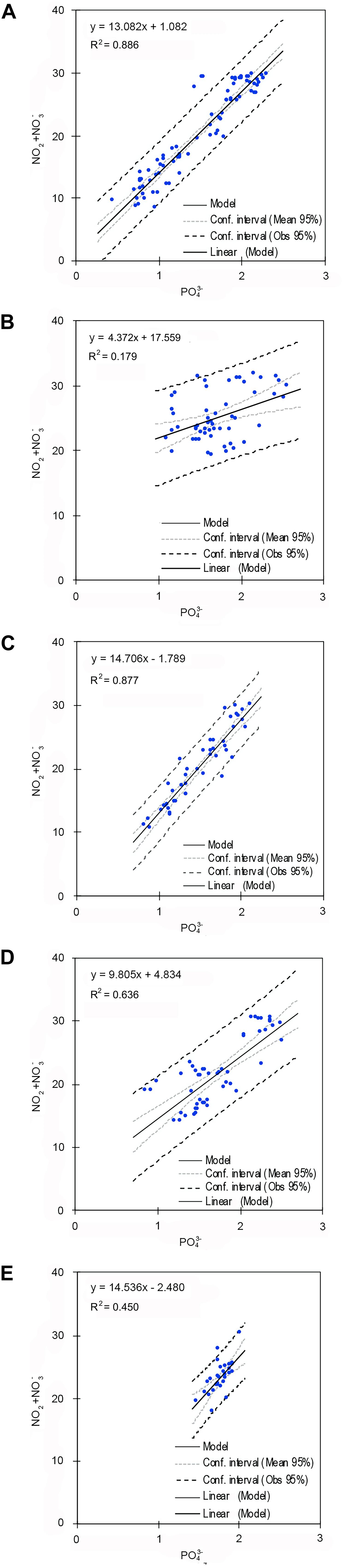
Figure 12. Correlation between nitrate + nitrite and phosphate for each sub-systems sampled: Area (A) 1, Area 2 (B), Area 3a (C), Area 3b (D), Area 4 (E).
This overall picture, together with data emerging from repeated stations, highlights the productivity and dynamism of TNB. By also taking into account previous studies, TNB appears to be characterized by a recurrent stratification of the water column during summer with large accumulation of biomass within UML and repeated blooms. The net dominance of diatoms we found agrees with several studies (e.g., Saggiomo et al., 2002; Mangoni et al., 2004, 2017; Fonda Umani et al., 2005; Rivaro et al., 2012), but differs to that reported by Mangoni et al. (2019), who observed an intense colonial P. antarctica summer bloom in stratified coastal waters of TNB. In this sense, the high productivity of UML during summer could be sustained by melting processes as well as episodic events that cause short-lived variations in the main environmental factors, contributing to the nutrient enrichment and fueling the species present within this layer (Bromwich and Kurtz, 1984; Kurtz and Bromwich, 1985; Arrigo et al., 2000; Mack et al., 2017).
Regarding Area 2, results cannot be compared with those of previous studies owing to the lack of previous data. However, productivity differences with TNB demonstrate even more clearly that phytoplankton growth and biomass accumulation within polynyas areas are higher than in adjacent waters (Arrigo and van Dijken, 2003), also in coastal systems and during the summer. Nutrients were not fully depleted in both areas and the net nutrient utilization (estimated by subtracting the nutrient concentration measured in UML from that measured in the deeper layers) was as those previously found for TNB (Rivaro et al., 2012, 2019). The differences found between Area 1 and 2 cannot be caused by different iron input, because the ranges measured for this micronutrient were comparable, even if the mean value in Area 1 was slightly higher than that in Area 2. Furthermore, dissolved iron concentrations were comparable with values reported for Antarctic coastal waters, reflecting the iron input either from land or from ice melting (Rivaro et al., 2019). Thus, taking into account all datasets and previous studies, we are inclined to consider that UML depth could probably regulate the productivity level rather than the net dominance of functional groups.
Compared to other sub-systems, the south-central Ross Sea (Area 3) exhibited biomass levels similar to those of TNB, especially Area 3b, showing a marked short-term variability in chemical and physical properties of the water column, as well as in percentages of functional groups. In Area 3a, the mean chl a was 104 mg chl a m–2, and P. antarctica displayed similar abundance to diatoms (46.03 and 42.05%, respectively). Meanwhile, in Area 3b, the mean chl a was 132 mg chl a m–2, and diatoms and P. antarctica represented 61.40 and 34.2% of the community, respectively. This shift was accompanied by a deepening of UML from 17 ± 10 m (Area 3a) to 56 ± 10 m depth (Area 3b) owing to atmosphere forcing, and by a different slope of [(NO3 + NO2):PO4], being 14.70 (R2 = 0.877) in Area 3a, and 9.80 (R2 = 0.636) in Area 3b. PCAs suggest that changes in UML depth led to a redistribution of chl a and Si(OH)4, although diatoms and haptophytes were inversely correlated in both sub-areas. In particular, the distribution of active variables in Area 3a suggests the presence of high diatom percentages in UML, characterized by high temperature and low salinity. Chl a showed a rather homogeneous distribution between UML and deeper layers. Contrastingly, haptophytes were more abundant below than within UML. As concerns the Area 3b, the overall picture from PCA indicated the presence of higher chl a within UML, in presence of warmer temperature, and a relatively higher percentages of diatoms, although the distribution of the two functional groups did not shows a net separation with respect to UML.
Data from the repeated stations seem to confirm that biomass between Mawson Bank and Crary Bank was higher than that at station LTER_EU_IT_17-002-M in the north-central Ross Sea, part of Joides Basin. The south-central Ross Sea has been considered to be a high-nutrient, low-chlorophyll (HNLC) area during the summer (El-Sayed, 1987; Nelson and Tréguer, 1992; Tréguer and Jacques, 1992; DiTullio and Smith, 1996; Smith et al., 1996; Saggiomo et al., 2002) although the timing of this condition strongly varies among years, and the bloom amplitude tended to increase since 2002 (Park et al., 2019). Early studies between 1990 and 1992 reported values of chl a reaching 3.1 μg L–1 in mid-January that decreased markedly by mid-February (Smith et al., 1996), while others have reported maximum values close to 1 μg L–1 in mid-late January 1996 (Saggiomo et al., 2002). In 2001, Mangoni et al. (2004), reported an integrated value of 102 mg chl a m–2 in late January at station 59 of this study, with a maximum of 1.78 μg L–1 with summer ice-coverage. In summer 2011, Kohut et al. (2017) reported a diatom bloom with chl a concentration exceeding 15 μg L–1 in presence of a UML of about 40 m depth over the Pennell Bank. In 2014, Mangoni et al. (2017) reported concentrations up to 202 mg chl a m–2 in the south-central Ross Sea in late January, with a maximum of 4.71 μg L–1 and a UML about 48 m deep and a net dominance of diatoms. The high biomass concentrations reported in this study confirm those reported by Park et al. (2019), providing additional information on the timing of productivity and temporal and spatial variability in the central Ross Sea at different scales during summer.
Area 4 was completely different to other sub-systems. This aspect is highlighted by PCA, showing the decoupling between UML and temperature/salinity, and the non-inverse correlation between haptophytes, diatoms, and chl a depict a completely different arrangement of variables of this sub-systems compared to those of the rest. Biomass and UML depth showed a pronounced variation between the southern and northern part, with chl a values ranging from 106.80 to 6.63 mg chl a m–2 at stations located on the continental shelf and those in the northern part, respectively, while UML depth ranged from 45 to 90 m (in the South and North, respectively). The lowest biomass level was found at stations that interface with the open Southern Ocean system, where bathymetry exceeds 2,000 m. This should be taken into account as Reddy and Arrigo (2006), who reported that the spring bloom duration in the Ross Sea is linked to the underlying bank and trough bathymetry of the outer shelf. The slope of [(NO3 + NO2):PO4] was 14.53 (R2 = 0.450), displaying lower variability than those of other areas and a lower nutrient utilization than those of coastal areas (Figure 12). The community was mainly dominated by diatoms, but dinoflagellates were the second most abundant group representing 40% of total biomass in some stations. The presence of dinoflagellates in this area was also reported by Mangoni et al. (2004), although with lower percentages. Dinoflagellates include mixotrophic forms (Gast et al., 2018) and have been reported in the Ross Sea by several authors in both spring and summer, although they are considered to have a minor role on the Antarctic food web and biogeochemistry (Stoecker et al., 1995; DiTullio and Smith, 1996; Phan-Tan et al., 2018). In addition, an intense bloom of loricate choanoflagellates in the central Ross Sea has been reported by Escalera et al. (2019) and a discovery of a novel dinoflagellate species (Prorocentrum sp.) associated with mucilaginous Phaeocystis antarctica colonies has been reported by Bolinesi et al. (2020). Therefore, these findings could help to reevaluate the role of the planktonic mixotrophic and heterotrophic compartment in the Antarctic food web, also in relation with recently reported changes within phytoplankton communities (e.g., Montes-Hugo et al., 2009; Kaufman et al., 2017; Mangoni et al., 2019).
Furthermore, data from repeated stations showed an increased chl a concentration at Mooring G station on February 9, with values ∼1.8 μg L–1 in the first 100 m and low phaeo:chl a ratios, which suggested the absence of grazers and an active phytoplankton biomass growth. Thus, some considerations must be made to explain the chl a concentration distribution and variation in relation to, not only to the availability of nutrients, but also the factors regulating grazing influence and the biological fate of the population. A synthetic representation of this ecological dynamic is shown in Figures 5, 7. Although the dominance of large cells was reported in all sub-systems, the percentages of micro- and nano-phytoplankton were similar in Area 1 and Area 4 (the most and least productive sub-areas, respectively). These data were accompanied by a different phaeo:chl a ratio, which indicated the similarity between classes could be a consequence of high removal by grazers in Area 1.
Conclusion
Besides the results presented in the section “Discussion,” some aspects of more general importance have emerged by our activity in Antarctica that deserve to be remarked. The Ross Sea phytoplankton communities have so far been considered as driven by the seasonal dynamics of the polynya, depicting the classical Antarctic food web. However, in addition to polynyas, others sub-systems are present, which follow alternative pathways for the primary production mechanisms. For example, the high percentage of dinoflagellates near Cape Adare and bloom of choanoflagellates in the central Ross Sea (Escalera et al., 2019) could lead to the reevaluation of the role of the planktonic mixotrophic and heterotrophic compartment in the trophodynamics of this region. The relative high biomass levels in polynya areas, together with diatom and micro-phytoplankton dominance, contrast with the HNLC feature of this area during summer (Sedwick et al., 2000). Diatoms dominated the community and reached higher percentage in occurrence with high concentration of chl a, with UML depth seeming to influence the biomass level rather than the dominance of different functional groups. This general picture points to an active accumulation of primary biomass in the upper levels of the water column, while phaeopigments, as indicators of different mechanisms of consumption, increased only in the lower parts of the water column. The high variability in timing of production and physical constraints of different sub-systems, highlights the importance to include areas interfacing with continental inputs and off-shore waters of the Southern Ocean in understanding the ecological dynamics of the Ross Sea, as well as the importance of L-TER sites in the study of such a critical system for the global carbon cycle. Thus, we believe that the information reported herewith contributes to understanding phytoplankton dynamics, which should be considered not only for marine physical and biological forcing, but, in a more general perspective, as a precious monitoring tool of the already ongoing climatic changes.
Data Availability Statement
The raw data supporting the conclusions of this article will be made available by the authors, without undue reservation, to any qualified researcher.
Ethics Statement
All samples were obtained during the projects in the framework of the Italian National Antarctic Program (PNRA16_00239; PNRA16_00207) coordinated by the Ministry of Education, University and Research (MIUR). The permission to collect samples was authorized by the National Environmental Officer of the National Agency for New Technologies, Energy and the Sustainable Economic Development (ENEA) on the base of Environmental Evaluation (Impact) Assessment of the Project, following the “Protocol on Environmental Protection of the Antarctic Treaty,” Annex II, art. 3.
Author Contributions
OM, PR, and VS designed the study. OM, FA, PC, AC, and PR carried out fieldwork. FB, MS, FA, PC, AC, GF, PR, and OM contributed to the laboratory measurements, data analysis, and interpreted the data. FB performed the statistical analysis. FB and OM wrote the manuscript with input and approval from all co-authors. VS contributed to the article conceptualization. All authors contributed to the article and approved the submitted version.
Funding
This study was funded by the Italian National Program for Antarctic Research, in the framework of the Projects P-ROSE (PNRA16_00239) and CELEBeR (PNRA16_00207).
Conflict of Interest
The authors declare that the research was conducted in the absence of any commercial or financial relationships that could be construed as a potential conflict of interest.
Acknowledgments
We express our gratitude to Italian Antarctic National Program (PNRA) and the scientific personnel and crew of the research vessel Italica for logistical support. We are also grateful to CoNISMa for general and continuous administrative support. We are grateful to Antonino De Natale for the support in Italy and invaluable efforts during the field activity and Gianluca Zazo for sampling during the cruise. We thank Augusto Passarelli for nutrient analysis of project P-ROSE. We wish to thank the kind collaboration of Prof. Gian Carlo Carrada, for his valuable criticism and constructive comments during the phase of manuscript writing. We would thank the reviewers for their constructive comments toward improving the manuscript.
Supplementary Material
The Supplementary Material for this article can be found online at: https://www.frontiersin.org/articles/10.3389/fmars.2020.574963/full#supplementary-material
Footnotes
References
Alderkamp, A.-C., Kulk, G., Buma, A. G. J., Visser, R. J. W., Van Dijken, G. L., Mills, M. M., et al. (2012). The effect of iron limitation on the photophysiology of Phaeocystis antarctica (Prymnesiophyceae) and Fragilariopsis cylindrus (Bacillariophyceae) under dynamic irradiance. J. Phycol. 48, 45–59. doi: 10.1111/j.1529-8817.2011.01098.x
Andreoli, C., Tolomio, C., Moro, I., Radice, M., Moschin, E., and Bellato, S. (1995). Diatoms and dinoflagellates in Terra Nova Bay (Ross Sea-Antarctica) during austral summer 1990. Polar Biol. 15, 465–475. doi: 10.1007/BF00237460
Arrigo, K. R., DiTullio, G. R., Dunbar, R. B., Robinson, D. H., vanWoert, M., Worthen, D. L., et al. (2000). Phytoplankton taxonomic variability in nutrient utilization and primary production in the Ross Sea. J. Geophys. Res. 105, 8827–8846. doi: 10.1029/1998JC000289
Arrigo, K. R., and McClain, C. R. (1994). Spring phytoplankton production in the western Ross Sea. Science 266, 261–263. doi: 10.1126/science.266.5183.261
Arrigo, K. R., Mills, M. M., Kropuenske, L. R., Van Dijken, G. L., Alderkamp, A.-C., and Robinson, D. H. (2010). Photophysiology in two major Southern Ocean taxa: photosynthesis and growth of Phaeocystis antarctica and Fragilariopsis cylindrus under different irradiance levels. Integr. Comp. Biol. 50, 950—966. doi: 10.1093/icb/icq021
Arrigo, K. R., Robinson, D. H., Worthen, D. L., Dunbar, R. B., DiTullio, G. R., van Woert, M., et al. (1999). Phytoplankton community structure and the drawdown of nutrients and CO2 in the Southern Ocean. Science 283, 365–367. doi: 10.1126/science.283.5400.365
Arrigo, K. R., and van Dijken, G. L. (2003). Phytoplankton dynamics within 37 Antarctic coastal polynya systems. J. Geophys. Res. 108:3271. doi: 10.1029/2002JC001739
Arrigo, K. R., van Dijken, G. L., and Bushinsky, S. (2008a). Primary production in the Southern Ocean, 1997–2006. J. Geophys. Res. 113:C08004. doi: 10.1029/2007JC004578
Arrigo, K. R., van Dijken, G. L., and Long, M. (2008b). Coastal Southern Ocean: a strong anthropogenic CO2 sink. Geophys. Res. Lett. 35:L21602. doi: 10.1029/2008GL035624
Arrigo, K. R., Worthen, D. L., Schnell, A., and Lizotte, M. P. (1998). Primary production in Southern Ocean waters. J. Geophys. Res. 103, 587–600. doi: 10.1029/98JC00930
Bender, S. J., Moran, D. M., McIlvin, M. R., Zheng, H., McCrow, J. P., Badger, J., et al. (2018). Colony formation in Phaeocystis antarctica: connecting molecular mechanisms with iron biogeochemistry. Biogeosciences 15, 4923–4942. doi: 10.5194/bg-15-4923-2018
Bertrand, E. M., Saito, M. A., Rose, J. M., Riesselman, C. R., Lohan, M. C., Noble, A. E., et al. (2007). Vitamin B12 and iron co-limitation of phytoplankton growth in the Ross Sea. Limnol. Oceanogr. 52, 1079–1093. doi: 10.4319/lo.2007.52.3.1079
Bolinesi, F., Saggiomo, M., Aceto, S., Cordone, A., Serino, E., Valoroso, M. C., et al. (2020). On the Relationship between a Novel Prorocentrum sp. and Colonial Phaeocystis antarctica under Iron and Vitamin B12 limitation: ecological implications for antarctic waters. Appl. Sci. 10:6965. doi: 10.3390/app10196965
Bromwich, D. H., and Kurtz, D. D. (1984). Katabatic wind forcing of the Terra Nova Bay polynya. J. Geophys. Res. 89, 3561–3572. doi: 10.1029/JC089iC03p03561
Brunet, C., and Mangoni, O. (2010). “Determinazione quali-quantitativa dei pigmenti fitoplanctonici mediante HPLC,” in Metodologie di Studio del Plancton marino, Vol. 56, eds G. Socal, I. Buttino, M. Cabrini, O. Mangoni, A. Penna, and C. Totti, (Roma: Ispra), 379–385.
Budillon, G., Castagno, P., Aliani, S., Spezie, G., and Padman, L. (2011). Thermohaline variability and Antarctic bottom water formation at the Ross Sea shelf break. Deep Sea Res. I 1002–1018. doi: 10.1016/j.dsr.2011.07.002
Caldeira, K., and Duffy, P. B. (2000). The role of the Southern Ocean in uptake and storage of anthropogenic carbon dioxide. Science 287, 620—622. doi: 10.1126/science.287.5453.620
Caron, D. A., Dennett, M. R., Lonsdale, D. J., Moran, D. M., and Shalapyonok, L. (2000). Microzooplankton herbivory in the Ross Sea, Antarctica. Deep Sea Res. II 47, 3249–3272.
Carter, L., Mccave, I., and Williams, M. (2008). Chapter 4. Circulation and water masses of the southern ocean: a review. Dev. Earth Environ. Sci. 8, 85–114. doi: 10.1016/S1571-9197(08)00004-9
Castagno, P., Capozzi, V., DiTullio, G. R., Falco, P., Fusco, G., Rintoul, S. R., et al. (2019). Rebound of shelf water salinity in the Ross Sea. Nat. Commun. 10:5441. doi: 10.1038/s41467-019-13083-8
Catalano, G., Budillon, G., La Ferla, R., Povero, P., Ravaioli, M., Saggiomo, V., et al. (2010). “The Ross Sea,” in Carbon and Nutrient Fluxes in Continental Margins: A Global Synthesis. Part II(Global Change: The IGBP Series), eds K.-K. Liu, L. Atkinson, R. Quinϸones, and L. Talaue-McManus, (Berlin: Springer Verlag), 303–318.
Collos, Y., Husseini-Ratrema, J., Bec, B., Vaquer, A., Lam Hoai, T., Rougier, C., et al. (2005). Pheopigment dynamics, zooplankton grazing rates and the autumnal ammonium peak in a Mediterranean lagoon. Hydrobiologia 550, 83–93.
Constable, A. J., Melbourne-Thomas, J., Corney, S. P., Arrigo, K. R., Barbraud, C., Barnes, D. K., et al. (2014). Climate change and Southern Ocean ecosystems I: how changes in physical habitats directly affect marine biota. Glob. Chang. Biol. 20, 3004–3025. doi: 10.1111/gcb.12623
Cullen, J., and Davis, R. F. (2003). The blank can make a big difference in oceanographic measurements. Limnol. Oceanogr. Bull. 12, 29–35. doi: 10.1002/lob.200312229
Dennett, M. R., Mathot, S., Caron, D. A., Smith, W. O. Jr., and Lonsdale, D. (2001). Abundance and distribution of phototrophic and heterotrophic nano- and microplankton in the Southern Ross Sea. Deep Sea Res. II 48, 4019–4037. doi: 10.1016/S0967-0645(01)00079-0
Deppeler, S. L., and Davidson, A. T. (2017). Southern ocean phytoplankton in a changing climate. Front. Mar. Sci. 4:40. doi: 10.3389/fmars.2017.00040
DiTullio, G. R., Geesey, M. E., Leventer, A. R., and Lizotte, M. P. (2003). “Algal pigment ratios in the Ross Sea: implications for CHEMTAX analysis of Southern Ocean data,” in Biogeochemistry of the Ross Sea. Antarctic Research Series 78, eds G. R. DiTullio and R. B. Dunbar, (Washington, DC: American Geophysical Union), 279–293.
DiTullio, G. R., Grebmeier, J., Arrigo, K. R., Lizotte, M. P., Robinson, D. H., Leventer, A., et al. (2000). Rapid and early export of Phaeocystis antarctica blooms in the Ross Sea, Antarctica. Nature 404, 595–598. doi: 10.1038/35007061
DiTullio, G. R., and Smith, W. O. Jr. (1996). Spatial patterns in phytoplankton biomass and pigment distributions in the Ross Sea. J. Geophys. Res. 101, 18467–18477. doi: 10.1029/96JC00034
Elliott, D. T., Tang, K. W., and Shields, A. R. (2009). Mesozooplankton beneath the summer sea ice in McMurdo Sound, Antarctica: abundance, species composition, and DMSP content. Polar Biol. 32, 113–122. doi: 10.1007/s00300–008-0511-3
El-Sayed, S. Z. (1987). “Biological productivity of Antarctic waters: present paradoxes and emerging paradigms,” in Antarctic Aquatic Biology, eds S. Z. El-Sayed and A. P. Tomo, (Cambridge: SCAR), 1–21.
Escalera, L., Mangoni, O., Bolinesi, F., and Saggiomo, M. (2019). Austral summer bloom of loricate choanoflagellates in the central Ross Sea Polynya. J. Eukaryot. Microbiol. 66, 849–852. doi: 10.1111/jeu.12720
Feng, Y., Hare, C. E., Rose, J. M., Handy, S. M., DiTullio, G. R., Lee, P. A., et al. (2010). Interactive effects of iron, irradiance and CO2 on Ross Sea phytoplankton. Deep Sea Res. I 57, 368–383. doi: 10.1016/j.dsr.2009.10.013
Fonda Umani, S., Monti, M., Bergamasco, A., Cabrini, M., De Vittor, C., Burba, N., et al. (2005). Plankton community structure and dynamics versus physical structure from Terra Nova Bay to Ross Ice Shelf (Antarctica). J. Mar. Syst. 55, 31–46. doi: 10.1016/j.jmarsys.2004.05.030
Franck, V. M., Brzezinski, M. A., Coale, K. H., and Nelson, D. M. (2000). Iron and silicic acid concentrations regulate Si uptake north and south of the Polar Frontal Zone in the Pacific Sector of the Southern Ocean. Deep Sea Res. II 47, 3315–3338. doi: 10.1016/S0967-0645(00)00070–9
Garcia, N. S., Sedwick, P. N., and DiTullio, G. R. (2009). Influence of irradiance and iron on the growth of colonial Phaeocystis antarctica: implications for seasonal bloom dynamics in the Ross Sea, Antarctica. Aquat. Microb. Ecol. 57, 203–220.
Gast, R. J., Scott, F. A., and Sanders, W. R. (2018). Mixotrophic activity and diversity of Antarctic marine Protists in Austral Summer. Front. Mar. Sci. 5:13. doi: 10.3389/fmars.2018.00013
Gibson, J. A. E., Garrick, R. C., Burton, H. R., and McTaggart, A. R. (1990). Dimethylsulfide and the alga Phaeocystis poucheti in Antarctic coastal waters. Mar. Biol. 104, 339–346.
Gruber, N., Landschützer, P., and Lovenduski, N. S. (2019). The variable southern ocean carbon sink. Annu. Rev. Mar. Sci. 11, 159–186. doi: 10.1146/annurev-marine-121916-063407
Hansen, H. P., and Grasshoff, K. (1983). “Automated chemical analysis,” in Methods of Seawater Analysis, eds K. Grasshoff, M. Ehrardt, and K. Kremlin, (Weinheim: Verlag-Chemie), 347–379.
Holm-Hansen, O., Lorenzen, C. J., Holmes, R. W., and Strickland, J. D. H. (1965). Fluorometric determination of chlorophyll. J. Conseil Permanent Int. Explor. Mer. 30, 3–15.
Iudicone, D., Rodgers, K. B., Stendardo, I., Aumont, O., Madec, G., Bopp, L., et al. (2011). Water masses as a unifying framework for understanding the Southern Ocean Carbon Cycle. Biogeosciences 8, 1031–1052.
Iudicone, D., Speich, S., Madec, G., and Blanke, B. (2008). The global conveyor belt from a southern ocean perspective. J. Phys. Oceanogr. 38, 1401–1425. doi: 10.1175/2007JPO3525.1
Jacobs, S. (2004). Bottom water production and its links with the thermohaline circulation. Antarctic Sci. 16, 427–437. doi: 10.1017/S095410200400224X
Jacobs, S. S., Amos, A. F., and Bruchhausen, P. M. (1970). Ross Sea oceanography and Antarctic bottom water formation. Deep Sea Res. Oceanogr. Abstr. 17, 935–962. doi: 10.1016/0011-7471(70)90046-X
Jacobs, S. S., Giulivi, C. F., and Mele, P. A. (2002). Freshening of the Ross Sea during the late 20th century. Science 297, 386–389. doi: 10.1126/science.1069574
Kaufman, D. E., Friedrichs, M. A. M., Smith, W. O. Jr., Hofmann, E. E., Dinniman, M. S., and Hemmings, J. C. P. (2017). Climate change impacts on southern Ross Sea phytoplankton composition, productivity, and export. J. Geophys. Res. 122, 2339–2359. doi: 10.1002/2016JC012514
Koch, F., Marcoval, M. A., Panzeca, C., Bruland, K. W., Sañudo-Wilhelmy, S. A., and Gobler, C. J. (2011). The effect of vitamin B12 on phytoplankton growth and community structure in the Gulf of Alaska. Limnol. Oceanogr. 56, 1023–1034. doi: 10.4319/lo.2011.56.3.1023
Kohut, J. T., Kustka, A. B., Hiscock, M., Lam, P. J., Measures, C., Milligan, A., et al. (2017). Mesoscale variability of the summer bloom over the northern Ross Sea shelf: a tale of two banks. J. Mar. Syst. 166, 50—60. doi: 10.1016/j.jmarsys.2016.10.010
Kurtz, D. D., and Bromwich, D. H. (1985). “A recurring, atmospherically forced polynya in Terra Nova Bay,” in Oceanology of the Antarctic Continental Shelf, Antarctic Series 43, ed. S. S. Jacobs, (Washington, DC: American Geophysical Union), 177–201.
Liu, X., and Smith, W. O. Jr. (2012). Physiochemical controls on phytoplankton distributions in the Ross Sea, Antarctica. J. Mar. Syst. 94, 135–144. doi: 10.1016/j.jmarsys.2011.11.013
Lonsdale, D. J., Caron, D. A., Dennett, M. R., and SchaVner, R. (2000). Predation by Oithona spp. on protozooplankton in the Ross Sea, Antarctica. Deep Sea Res. II 47, 3273–3283. doi: 10.1016/S0967-0645(00)00068-0
Mack, S. L., Dinniman, M. S., McGillicuddy, D. J. Jr., Sedwick, P. N., and Klinck, J. M. (2017). Dissolved iron transport pathways in the Ross Sea: influence of tides and horizontal resolution in a regional ocean model. J. Mar. Syst. 166, 73–78. doi: 10.1016/j.jmarsys.2016.10.008
Mackey, M. D., Mackey, D. J., Higgin, H. W., and Wright, S. W. (1996). CHEMTAX-a program for estimating class abundances from chemical markers: application to HPLC measurements of phytoplankton. Mar. Ecol. Progr. Ser. 144, 265–283.
Mangoni, O., Modigh, M., Conversano, F., Carrada, G. C., and Saggiomo, V. (2004). Effects of summer ice coverage on phytoplankton assemblages in the Ross Sea, Antarctica. Deep Sea Res. I 51, 1601–1617. doi: 10.1016/j.dsr.2004.07.006
Mangoni, O., Saggiomo, M., Bolinesi, F., Castellano, M., Povero, P., Saggiomo, V., et al. (2019). Phaeocystis antarctica unusual summer bloom in stratified Antarctic coastal waters (Terra Nova Bay, Ross Sea). Mar. Environ. Res. 151:104733. doi: 10.1016/j.marenvres.2019.05.012
Mangoni, O., Saggiomo, M., Modigh, M., Catalano, G., Zingone, A., and Saggiomo, V. (2009). The role of platelet ice microalgae in seeding phytoplankton blooms in Terra Nova Bay (Ross Sea, Antarctica): a mesocosm experiment. Polar Biol. 3, 311–323. doi: 10.1007/s00300–008-0507-z
Mangoni, O., Saggiomo, V., Bolinesi, F., Escalera, L., and Saggiomo, M. (2018). A review of past and present summer primary production processes in the Ross Sea in relation to changing ecosystems. Ecol. Quest. 29, 75–85. doi: 10.12775/EQ.2018.024
Mangoni, O., Saggiomo, V., Bolinesi, F., Margiotta, F., Budillon, G., Cotroneo, Y., et al. (2017). Phytoplankton blooms during austral summer in the Ross Sea, Antarctica: driving factors and trophic implications. PLoS One 12:e0176033. doi: 10.1371/journal.pone.0176033
Mathiot, P., Jourdain, N. C., Barnier, B., Galleìe, H., Molines, J. M., Le Sommer, J., et al. (2012). Sensitivity of coastal polynyas and high-salinity shelf water production in the Ross Sea, Antarctica, to the atmospheric forcing. Ocean Dyn. 62, 701–723. doi: 10.1007/s10236-012-0531-y
Maxwell, K., and Johnson, G. N. (2000). Chlorophyll fluorescence – a practical guide. J. Exp. Bot. 51, 659–668. doi: 10.1093/jexbot/51.345.659
Misic, C., Covazzi Harriague, A., Mangoni, O., Cotroneo, Y., Aulicino, G., and Castagno, P. (2017). Different responses of the trophic features of particulate organic matter to summer constraints in the Ross Sea. J. Mar. Syst. 166, 132–143. doi: 10.1016/j.jmarsys.2016.06.012
Montes-Hugo, M., Doney, S. C., Ducklow, H. W., Fraser, W., Martinson, D., and Stammerjohn, S. E. (2009). Recent changes in phytoplankton communities associated with rapid regional climate change along the Western Antarctic Peninsula. Science 323, 1470—1473. doi: 10.1126/science.1164533
Montes-Hugo, M. A., and Yuan, X. (2012). Climate patterns and phytoplankton dynamics in Antarctic latent heat polynyas. J. Geophys. Res. 117:C05031. doi: 10.1029/2010JC006597
Nelson, D. M., and Tréguer, P. (1992). Role of silicon as a limiting nutrient to Antarctic diatoms: evidence from kinetic studies in the Ross Sea ice-edge zone. Mar. Ecol. Progr. Ser. 80, 255–264. doi: 10.3354/meps080255
Orsi, A. H., Johnson, G. C., and Bullister, J. L. (1999). Circulation, mixing and production of Antarctic bottom water. Progr. Oceanogr. 43, 55–109. doi: 10.1016/S0079-6611(99)00004-X
Orsi, A. H., and Wiederwohl, C. L. (2009). A recount of Ross Sea waters. Deep Sea Res. II 56, 778–795. doi: 10.1016/j.dsr2.2008.10.10.033
Park, J., Kim, J.-H., Kim, H.-C., Hwang, J., Jo, Y.-H., and Lee, S. H. (2019). Environmental forcing on the remotely sensed phytoplankton bloom phenology in the central Ross Sea Polynya. J. Geophys. Res. Oceans 124, 5400—5417. doi: 10.1029/2019JC015222
Peloquin, J. A., and Smith, W. O. Jr. (2007). Phytoplankton blooms in the Ross Sea, Antarctica: interannual variability in magnitude, temporal patterns, and composition. J. Geophys. Res. 112:C08013. doi: 10.1029/2006JC003816
Phan-Tan, L., Nguyen-Ngoc, L., Smith, W., and Doan, H. (2018). A new dinoflagellate species, Protoperidinium smithii H. Doan-Nhu, L. Phan-Tan et L. Nguyen-Ngoc sp. nov., and an emended description of Protoperidinium defectum (Balech 1965) Balech 1974 from the Ross Sea, Antarctica. Polar Biol. 41, 983–992. doi: 10.1007/s00300–018-2262-0
Pinkerton, M. H., Bradford-Grieve, J. M., and Hanchet, S. M. (2010). A balanced model of the food web of the Ross Sea, Antarctica. CCAMLR Sci. 17, 1–31.
Reddy, T. E., and Arrigo, K. R. (2006). Constraints on the extent of the Ross Sea phytoplankton bloom. J. Geophys. Res. 111:C07005. doi: 10.1029/2005JC003339
Rivaro, P., Abelmoschi, M. L., Grotti, M., Ianni, C., Magi, E., Margiotta, F., et al. (2012). Combined effects of hydrographic structure and iron and copper availability on the phytoplankton growth in Terra Nova Bay Polynya (Ross Sea, Antarctica). Deep Sea Res. I 62, 97–110. doi: 10.1016/j.dsr.2011.12.008
Rivaro, P., Ardini, F., Grotti, M., Aulicino, G., Cotroneo, Y., Fusco, G., et al. (2019). Mesoscale variability related to iron speciation in a coastal Ross Sea area (Antarctica) during summer 2014. Chem. Ecol. 35, 1–19. doi: 10.1080/02757540.2018.1531987
Rivaro, P., Ianni, C., Langone, L., Ori, C., Aulicino, G., Cotroneo, Y., et al. (2017). Physical and biological forcing of mesoscale variability in the carbonate system of the Ross Sea (Antarctica) during summer 2014. J. Mar. Syst. 166, 144–158. doi: 10.1016/j.jmarsys.2015.11.002
Ryan-Keogh, T. J., DeLizo, L. M., Smith, W. O. Jr., Sedwick, P. N., McGillicuddy, D. J., Moore, C. M., et al. (2017). Temporal progression of photosynthetic strategy in phytoplankton in the Ross Sea, Antarctica. J. Mar. Syst. 166, 87–96. doi: 10.1016/j.jmarsys.2016.08.014
Saggiomo, V., Carrada, G. C., Mangoni, O., Ribera d’Alcalà, M., and Russo, A. (1998). Spatial and temporal variability of size fractionated biomass and primary production in the Ross Sea (Antarctica) during the austral spring and summer. J. Mar. Syst. 17, 115–127.
Saggiomo, V., Catalano, G., Mangoni, O., Budillon, G., and Carrada, G. C. (2002). Primary production processes in ice-free waters of the Ross Sea (Antarctica) during the austral summer 1996. Deep Sea Res. II 49, 1787–1801. doi: 10.1016/S0967-0645(02)00012-7
Saino, N., and Guglielmo, L. (2000). “ROSSMZE expedition: distribution and biomass of bird and mammals in the western Ross Sea,” in Ross Sea Ecology, Italian Antarctic expeditions (1987-1995), eds F. M. Faranda, L. Guglielmo, and A. Ianora, (Berlin: Springer), 469–478.
Schoemann, V., Becquevort, S., Stefels, J., Rousseau, V., and Lancelotte, C. (2005). Phaeocystis blooms in the global ocean and their controlling mechanisms: a review. J. Sea Res. 53, 43–66. doi: 10.1016/j.seares.2004.01.008
Sedwick, P. N., and DiTullio, G. R. (1997). Regulation of algal blooms in Antarctic shelf waters by the release of iron from melting sea ice. Geophys. Res. Lett. 24, 2515–2518. doi: 10.1029/97GL02596
Sedwick, P. N., DiTullio, G. R., and Mackey, D. J. (2000). Iron and manganese in the Ross Sea, Antarctica: seasonal iron limitation in Antarctic shelf waters. J. Geophys. Res. 105, 11321–11336. doi: 10.1029/2000JC000256
Sedwick, P. N., Marsay, C. M., Sohst, B. M., Aguilar-Islas, A. M., Lohan, M. C., Long, M. C., et al. (2011). Early season depletion of dissolved iron in the Ross Sea polynya: implications for iron dynamics on the Antarctic continental shelf. J. Geophys. Res. 116:C12019. doi: 10.1029/2010JC006553
Shuman, F. R., and Lorenzen, C. J. (1975). Quantitative degradation of chlorophyll by a marine herbivore. Limnol. Oceanogr. 20, 580—586.
Siegel, V. (2005). Distribution and population dynamics of Euphausia superba: summary of recent findings. Polar Biol. 29, 1–22. doi: 10.1007/s00300–005-0058-5
Silvano, A., Foppert, A., Rintoul, S. R., Holland, S. R., Tamura, T., Kimura, N., et al. (2020). Recent recovery of Antarctic Bottom Water formation in the Ross Sea driven by climate anomalies. Nat. Geosci. 10:5441. doi: 10.1038/s41561-020–00655-3
Smith, W. O. Jr., Ainley, D. G., Arrigo, K. R., and Dinniman, M. S. (2014). The oceanography and ecology of the Ross Sea. Annu. Rev. Mar. Sci. 6, 469–487. doi: 10.1146/annurev-marine-010213-135114
Smith, W. O. Jr., Ainley, D. G., and Cattaneo-Vietti, R. (2007). Trophic interactions within the Ross Sea continental shelf ecosystem. Philos. Trans. R. Soc. B 362, 95–111. doi: 10.1098/rstb.2006.1956
Smith, W. O. Jr., and Asper, V. (2001). The influence of phytoplankton assemblage composition on biogeochemical characteristics and cycles in the southern Ross Sea, Antarctica. Deep Sea Res. I 48, 137–161. doi: 10.1016/S0967-0637(00)00045-5
Smith, W. O. Jr., Carlson, C. A., Ducklow, H. W., and Hansell, D. A. (1998). Growth dynamics of Phaeocystis antarctica-dominated plankton assemblages from the Ross Sea. Mar. Ecol. Progr. Ser. 168, 229–244. doi: 10.3354/meps168229
Smith, W. O. Jr., Dinnimanm, M., Klinckm, J., and Hoffmannm, E. (2003). Biogeochemical climatologies in the Ross Sea, Antarctica: seasonal patterns of nutrients and biomass. Deep Sea Res. Part II 50, 3083–3101. doi: 10.1016/j.dsr2.2003.07.010
Smith, W. O. Jr., and Gordon, L. I. (1997). Hyperproductivity of the Ross Sea (Antarctica) polynya during austral spring. Geophys. Res. Lett. 24, 233–236. doi: 10.1029/96GL03926
Smith, W. O. Jr., and Jones, R. M. (2015). Vertical mixing, critical depths, and phytoplankton growth in the Ross Sea. ICES J. Mar. Sci. 72, 1952–1960. doi: 10.1093/icesjms/fsu234
Smith, W. O. Jr., Shields, A. R., Dreyer, J. C., Peloquin, J. A., and Asper, V. (2011). Interannual variability in vertical export in the Ross Sea: magnitude, composition, and environmental correlates. Deep Sea Res. I 58, 147–159. doi: 10.1016/j.dsr.2010.11.007
Smith, W. O. Jr., Shields, A. R., Peloquin, J. A., Catalano, G., Tozzi, S., Dinniman, M. S., et al. (2006). Interannual variations in nutrients, net community production, and biogeochemical cycles in the Ross Sea. Deep-Sea Res. II 53, 815–833. doi: 10.1016/j.dsr2.2006.02.014
Smith, W. O. Jr., Tozzi, S., DiTullio, G. R., Dinnimand, M., Mangoni, O., Modigh, M., et al. (2010). Phytoplankton photosynthetic pigments in the Ross Sea: patterns and relationships among functional groups. J. Mar. Syst. 82, 177–185. doi: 10.1016/j.jmarsys.2010.04.014
Smith, W. O., and Comiso, J. C. (2008). Influence of sea ice on primary production in the Southern Ocean: a satellite perspective. J. Geophys. Res. 113:C05S93. doi: 10.1029/2007JC004251
Smith, W. O., Nelson, D. M., DiTullio, G. R., and Leventer, A. R. (1996). Temporal and spatial patterns in the Ross Sea: phytoplankton biomass, elemental composition, productivity and growth rates. J. Geophys. Res. 101, 18455–18465. doi: 10.1029/96JC01304
Stoecker, D. K., Putt, M., and Moisan, T. (1995). Nano- and micro-plankton dynamics during the spring Phaeocystis sp. bloom in McMurdo Sound, Antarctica. J. Mar. Biol. Assoc. U.K. 75, 815–832. doi: 10.1017/S0025315400038170
Sweeney, C., Smith, W. O. Jr., Hales, B., Bidigare, R. R., Carlson, C. A., Codispoti, L. A., et al. (2000). Nutrient and carbon removal ratios and fluxes in the Ross Sea, Antarctica. Deep Sea Res. II 47, 3395–3421. doi: 10.1016/S0967-0645(00)00073-4
Tagliabue, A., and Arrigo, K. R. (2003). Anomalously low zooplankton abundance in the Ross Sea: an alternative explanation. Limnol. Oceanogr. 48, 686–699. doi: 10.4319/lo.2003.48.2.0686
Tamura, T., Ohshima, K. I., and Nihashi, S. (2008). Mapping of sea ice production for Antarctic coastal polynyas. Geophys. Res. Lett. 35:L07606. doi: 10.1029/2007GL032903
Tang, K. W., Smith, W. O. Jr., Elliot, D. T., and Schields, A. R. (2008). Colony size of Phaeocystis antarctica (Prymnesiophyceae) as influenced by zooplankton grazers. J. Phycol. 44, 1372–1378. doi: 10.1111/j.1529-8817.2008.00595.x
Tréguer, P., and Jacques, G. (1992). Review Dynamics of nutrients and phytoplankton, and fluxes of carbon, nitrogen and silicon in the Antarctic Ocean. Polar Biol. 12, 149–162. doi: 10.1007/BF00238255
Turner, J., Barrand, N. E., Bracegirdle, T. J., Convey, P., Hodgson, D. A., Jarvis, M., et al. (2013). Antarctic climate change and the environment: an update. Polar Rec. 50, 237–259. doi: 10.1017/S0032247413000296
Vidussi, F., Claustre, H., Bustillos-Guzman, J., Cailliau, C., and Marty, J. C. (1996). Determination of chlorophylls and carotenoids of marine phytoplankton: separation of chlorophyll a from divinylchlorophyll a and zeaxanthin from lutein. J. Plankton Res. 18, 2377–2382.
Williams, R. (1985). “Trophic relationships between pelagic fish and euphausiids in Antarctic waters,” in Antarctic Nutrient Cycles and Food Webs, eds W. R. Siegfried, P. R. Condy, and R. M. Laws, (Berlin: Springer-Verlag), 452–459.
Wright, S. W., van den Enden, R. L., Pearce, I., Davidson, A. T., Scott, F. J., and Westwood, K. J. (2010). Phytoplankton community structure and stocks in the Southern Ocean (30—80 E) determined by CHEMTAX analysis determined by HPLC pigment signatures. Deep Sea Res. II 57, 758–778.
Wu, J., and Boyle, E. A. (1998). Determination of iron in seawater by high resolution isotope dilution inductively coupled plasma mass spectrometry after Mg(OH)2 co-precipitation. Anal. Chim. Acta 367, 183–191. doi: 10.1016/S0003-2670(98)00145-7
Xavier, J. C., Brandt, A., Ropert-Coudert, Y., Badhe, R., Gutt, J., Havermans, C., et al. (2016). Future challenges in Southern ocean ecology research. Front. Mar. Sci. 3:94. doi: 10.3389/fmars.2016.00094
Keywords: phytoplankton functional groups, size classes, pigments, chemotaxonomy, quantum efficiency, grazing index, austral summer
Citation: Bolinesi F, Saggiomo M, Ardini F, Castagno P, Cordone A, Fusco G, Rivaro P, Saggiomo V and Mangoni O (2020) Spatial-Related Community Structure and Dynamics in Phytoplankton of the Ross Sea, Antarctica. Front. Mar. Sci. 7:574963. doi: 10.3389/fmars.2020.574963
Received: 22 June 2020; Accepted: 19 November 2020;
Published: 18 December 2020.
Edited by:
Elif Eker-Develi, Mersin University, TurkeyReviewed by:
Sergei Danchenko, University of Cádiz, SpainCarmelo Tomas, University of North Carolina at Wilmington, United States
Copyright © 2020 Bolinesi, Saggiomo, Ardini, Castagno, Cordone, Fusco, Rivaro, Saggiomo and Mangoni. This is an open-access article distributed under the terms of the Creative Commons Attribution License (CC BY). The use, distribution or reproduction in other forums is permitted, provided the original author(s) and the copyright owner(s) are credited and that the original publication in this journal is cited, in accordance with accepted academic practice. No use, distribution or reproduction is permitted which does not comply with these terms.
*Correspondence: Olga Mangoni, olga.mangoni@unina.it