The Abundance of Kelp Is Modified by the Combined Impact of Depth, Waves and Currents

Introduction

Kelp forests are found on rocky seabed in the temperate and Arctic parts of the world (Mann, 2000; Bartsch et al., 2008). Laminaria hyperborea is the dominating kelp species in the northeast Atlantic, distributed from Portugal (∼37°N; Kain, 1971b) to the Murman coast (∼68°N; Schoschina, 1997). Along the Norwegian coast, L. hyperborea cover large parts of the shallow (down to approx. 30 m depth) subtidal rocky seabed in wave exposed and moderately exposed areas (Kain, 1971b; Bekkby et al., 2009), except for the sea urchin grazed barrens in the northernmost parts (Norderhaug and Christie, 2009; Rinde et al., 2014). The L. hyperborea forests have high production (Abdullah and Fredriksen, 2004), function as habitat for many different species of algae and fauna (Whittick, 1983; Norderhaug et al., 2005) and provide a wide range of ecosystem services (Gundersen et al., 2016).

Several studies have documented the effect of environmental variables on recruitment, survival, growth, size, biomass and density of L. hyperborea kelp. Within the salinity and temperature tolerance limit (Kain, 1971a; Bolton and Lüning, 1982), nutrient and light are key factors (Graham et al., 2016). The depth at which the kelp grows determines the light influx whereas water flow impacts the nutrient transport across the boundary layer (Raven, 1981) and the degree of lamina fouling by epiphytic growth (Strand and Weisner, 1996; Pihl et al., 1999). Water flow is also associated with wounding, breakage, dislodgement (de Bettignies et al., 2012; Graham et al., 2016) and morphological changes due to drag-reducing adaptation (Armstrong, 1989). Water flow may come in the form of wave induced exposure or ocean currents, with wave exposure being more orbital than the unidirectional ocean currents, with a large tidal component (Miller et al., 2011). The effect of wave exposure on L. hyperborea distribution, growth, density, production, biomass, mortality and morphology has been documented in several studies (e.g., Svendsen and Kain, 1971; Sjøtun and Fredriksen, 1995; Sjøtun et al., 1998; Gorman et al., 2012; Pedersen et al., 2012). However, the effect of current speed has been less studied for L. hyperborea (but see Bekkby et al., 2009, 2014 and the discussion in Kain, 1971a).

Already decades ago, Kain (1971a) suggested different effects of high currents than high wave exposures on kelp morphology. Eckman et al. (2003), and later Bekkby et al. (2014), studied the relative importance of these two different types of water flow on kelp size and biomass and found that the combined influence of these two types of water flow is not just a matter of total water flow. The aim of the present study was therefore to analyze the combined impact of the two types of water flow, wave exposure and ocean currents, on kelp abundance, taking the effect of other important environmental variables, such as depth, terrain, slope, salinity and temperature, into account. One of our other studies (Bekkby et al., 2009), located in a small area off the West coast of Norway, found little impact of current speed on kelp distribution, which was partly explained by the narrow range of current speed covered in the study. Our present study includes a large dataset, covering a wide range of wave exposures and ocean current levels, as well as several ecoregions along the NE Atlantic (Norwegian) coast, both Skagerrak, the North Sea and the southern part of the Norwegian Sea, from 58°N to 66°N, thereby avoiding areas further north that for the last decades have been heavily grazed by sea urchins, Strongylocentrotus droebachiensis (in the northern part of the Norwegian Sea; Norderhaug and Christie, 2009; Rinde et al., 2014).

Materials and Methods

Study Area and Field Sampling

The National program for mapping biodiversity – coast (Bekkby et al., 2011) has since 2004 registered kelp (L. hyperborea) forest abundances all along the Norwegian coast, resulting in a dataset consisting of 6,445 observations from the Swedish border in the south (58°N) to Brønnøysund in the north (66°N), see Figure 1. Kelp abundance in the canopy layer (i.e., not including the understory) was recorded at georeferenced (using a handheld GPS) sites during the summer season (from May to September), with the use of water goggles (in the very shallow areas) and underwater cameras from small boats. Kelp canopy abundance was semi-quantitatively classified, observed from above the canopy, into four classes based on the National program protocol (Bekkby et al., 2015), where 0 = absence; 1 = single kelp and scarce, i.e., 1–2 kelps per m²; 2 = moderately dense, i.e., it is possible to see the seabed through the canopy, 2–8 kelps per m²; or 3 = dense, i.e., impossible to see the seabed through the canopy, typically 8–10 kelps per m². Only observations on rocky seabed (i.e., suitable substrate for kelp growth) and observations covered by the predictors (see chapters below) were included in the analyses, resulting in 2,517 data points on kelp abundance (Figure 1).

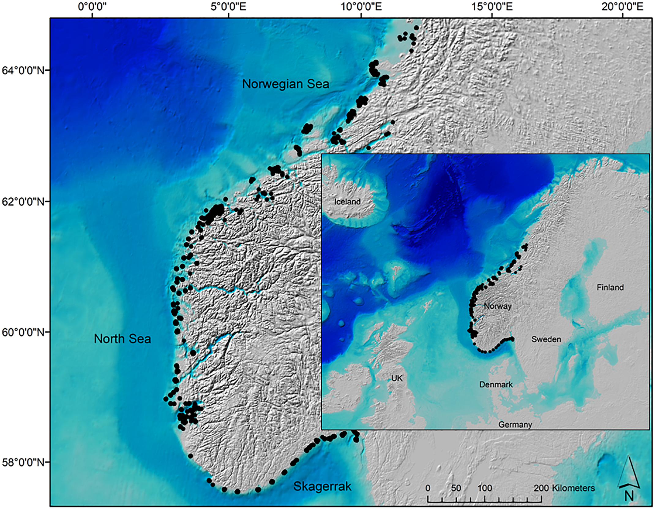
Figure 1. The study area covering the Skagerrak, the North Sea and the southern part of the Norwegian Sea, from 58°N to 66°N, with 2,517 observations (black dots) on kelp (Laminaria hyperborea) canopy abundance collected in the period 2004–2017. Background map: http://www.gebco.net.

Environmental Variables (Predictors)

Light, nutrient, salinity, temperature are all key factors for kelp growth (Kain, 1971a; Bolton and Lüning, 1982; Graham et al., 2016). Water flow impacts nutrient uptake, lamina fouling and the degree of wounding, breakage and dislodgement of the kelp (Raven, 1981; Strand and Weisner, 1996; Pihl et al., 1999; de Bettignies et al., 2012; Graham et al., 2016). Our observations on kelp canopy abundance were therefore linked to field measured data and models representing these factors. Depth was recorded in the field and serves as a finer-scaled proxy for light at the seabed than the modeled information. Information on light at the seabed, wave exposure, ocean currents, salinity and temperature were available as models. In order to capture smaller scaled differences in ocean currents than what is captured by the coarse ocean current model available, modeled terrain curvature was included. Steep slopes may provide challenges when it comes to the attachment of kelp, thus, modeled slope was also included in the analyses. More details on the environmental variables are provided below.

Wave exposure (m²/s) was modeled with a horizontal resolution of 25 m (Isæus, 2004) using data on wind speed and direction from the Norwegian Meteorological Institute, averaged over a 10-year period (1995–2004). The model has been applied in several research projects, both in Norway (e.g., Bekkby et al., 2009, 2014; Pedersen et al., 2012; Norderhaug et al., 2014; Rinde et al., 2014), Sweden (e.g., Eriksson et al., 2004), Finland (Isæus and Rygg, 2005), Denmark and the Baltic Sea (Wijkmark and Isæus, 2010).

Current speed (m/s), temperature (°C), and salinity (psu) were modeled at a horizontal resolution of 800 m (NorKyst-800; Albretsen et al., 2011) using the three-dimensional numerical ocean model ROMS (Regional Ocean Modeling System¹; Shchepetkin and McWilliams, 2005; Haidvogel et al., 2008). The model statistics were retrieved from two separate simulations averaged for the period January–August in 2013 and 2014. The model was forced by atmospheric surface fields from a high-resolution wind model (the Weather Research and Forecasting model; Skamarock et al., 2008), the global TPXO model (Egbert and Erofeeva, 2002) for the tidal forcing and daily averaged surface elevation, currents and hydrography from the operational forecast provided by the Norwegian Meteorological Institute (thredds.met.no). Mean values and 90th percentiles (i.e., the 10% highest values) for the seabed were used in our analyses.

Depth was recorded in the field at every site, either using the depth sensor on the underwater camera, or by using a handheld depth sensor (when water goggles were used). The depth values were standardized to lowest astronomical tide level (standard nautical chart zero), correcting for variation in total water level (i.e., both tidal elevation and storm surge) using data from the Norwegian Hydrographic Service. Time of day was lacking for 574 observations. However, as these were from an area where the tidal differences are low (south of 61.5°N, Møre og Romsdal County) the error introduced to the dataset is believed to be negligible, and these data were therefore still included in the analyses. Slope (°) and terrain curvature (m) were derived from a digital depth model with 25 m horizontal resolution, provided by the Norwegian Hydrographic Service. Terrain curvature was estimated with both a 250 m, 500 m and 1 km spatial calculation window (Bekkby et al., 2009). Light at the seabed (photosynthetically active radiation, PAR, E m^–2 d^–1) was modeled using data from ocean color satellite sensor estimates, with an algorithm improved for coastal waters as described in Saulquin et al. (2013) (averaged for the period 2009–2013 at 100 m horizontal resolution, as described in Populus et al., 2017). Combined with the depth model provided by the Norwegian Hydrographic Service, light at the seabed was down-scaled to a model with 25 m horizontal resolution.

Statistical Analyses

In order to avoid subjective evaluation of which environmental variables (predictors) should be transformed to achieve homogeneity of variances, all predictors were transformed to zero skewness at a 0–1 scale prior to the analyses (cf. Økland et al., 2003). For better visual interpretation of the response plots (Figures 2, 3), the predictor values were transformed back to original values. All analyses were carried out in R version 3.3.3 (R Development Core Team, 2017). We used cumulative link models (CLMs, Agresti, 2013), which is suitable to analyze ordinal response variables (R library: ordinal; Christensen, 2015). CLM is parallel to “ordinal regression models,” “continuation ratio models,” and “proportional odds models” (McCullagh, 1980) and are comparable to its linear or curved counterparts (e.g., Generalized Linear Models, GLMs). The predictors wave exposure, current speed (mean and 90pc), depth, slope, curvature (calculation windows of 250, 500, and 1000 m), light at the seabed, temperature, and salinity (mean and 90pc) were included in the analyses. Also, two interactions were included to test for possible depth-specific effects of wave exposure and wave-specific effects of current speed. To account for spatial autocorrelation, the interaction between latitude and longitude was included in the models, which is regarded as an appropriate way to capture spatial structures in non-linear methods (Legendre, 1993). Candidate models consisting of all possible combinations of the predictors were tested, and the best among them was selected using Akaike Information Criterion (AIC; Burnham et al., 2011). The model selection was carried out using the dredge function in the R library MuMIn (Bartón, 2018). Models with ΔAIC < 4 are considered almost equally good according to Burnham and Anderson (2002) and discussed as such.

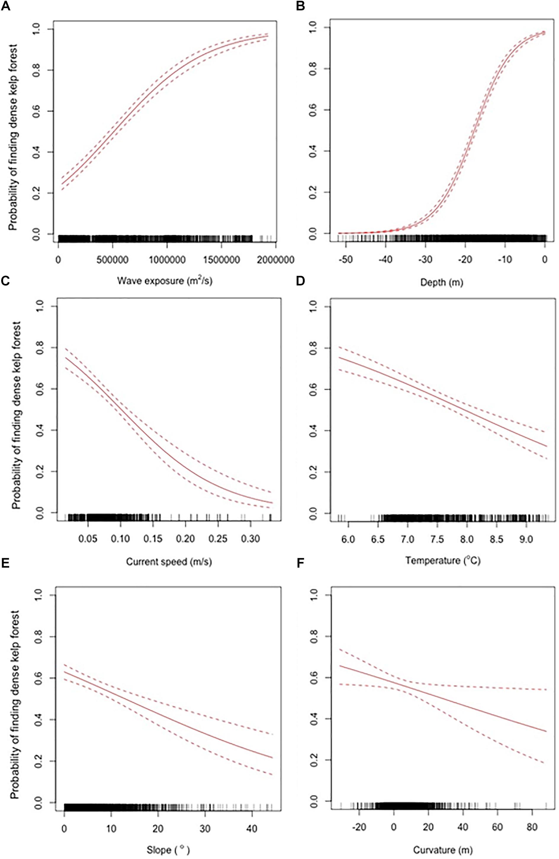
Figure 2. The probability of finding dense Laminaria hyperborea kelp forests (canopy kelp abundance class 3) as a function of wave exposure (A), depth (B), current speed (C), temperature (D), slope (E), and curvature (F), with the 95% confidence interval as a broken line. The black dots on the x-axis show the distribution of the data in the environmental variable space.

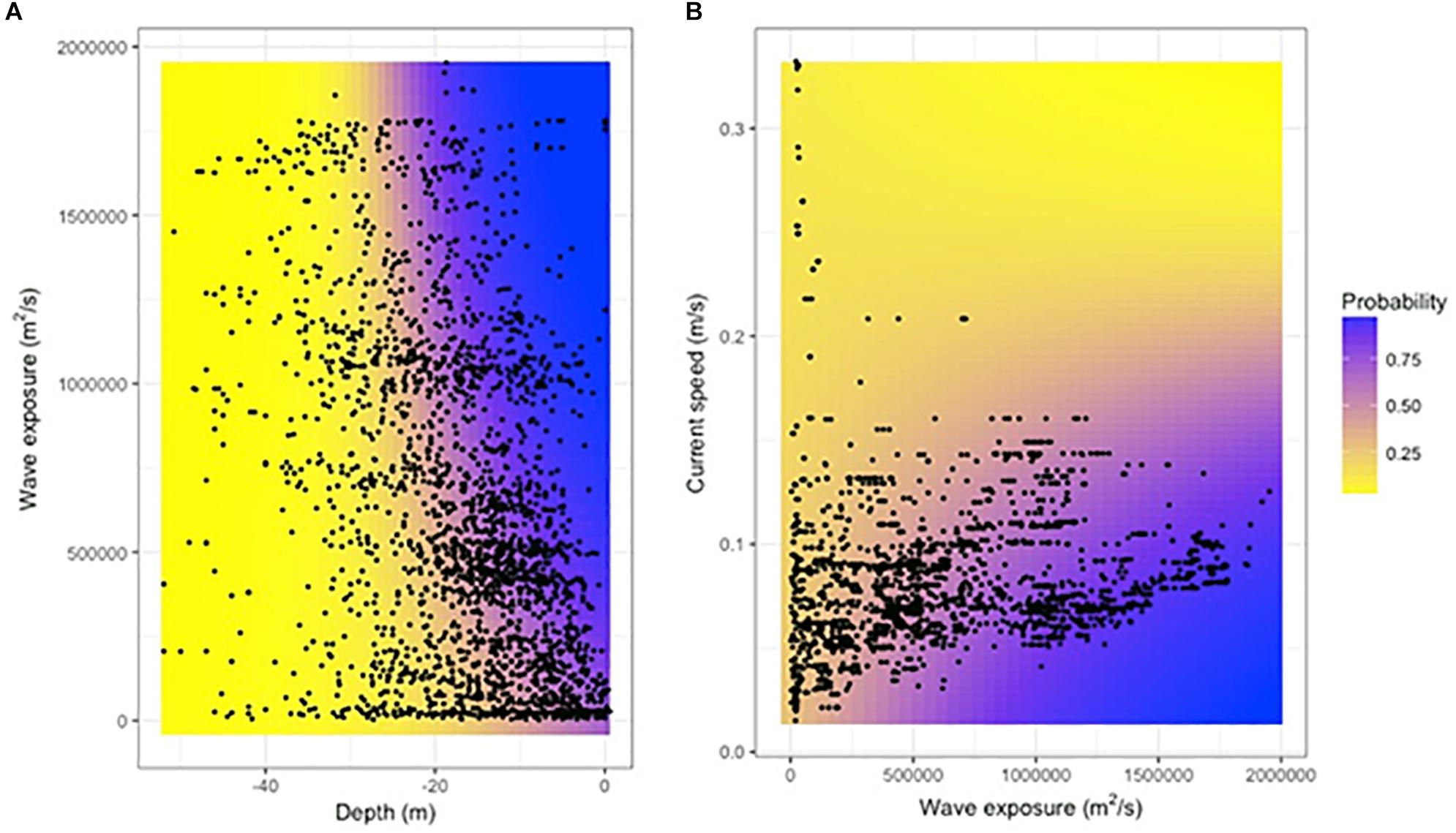
Figure 3. The probability of finding dense Laminaria hyperborea kelp forests (canopy kelp abundance class 3) as a function of the interaction between wave exposure and depth (A) and current speed and wave exposure (B). Blue coloring indicates high probability, yellow coloring indicates low probability. The black dots show the distribution of the data in the environmental space. The plots are made using the ggplot2 function in R (Wickham, 2009).

To avoid biases in the analyses caused by correlating predictors, only variables with Pearson’s r ≤ 0.5 were included in the same model. This limit is relatively strict and was chosen to reduce the number of predictors in the analyses, making the candidate models somewhat simpler. Four groups of correlated (r > 0.5) predictors were tested in separate models, so that the predictor explaining most of the variation was included in the modeling. These four groups consisted of the three curvature variables (r > 0.64) and mean and 90pc versions of ocean currents (r = 0.99), temperature (r = 0.97), and salinity (r = 0.88), respectively. Consequently, curvature with a 500 m spatial calculation window, mean values of temperature and current speed and the 90th percentile of salinity were selected to be included in the model testing. For the same reason, depth (which is a proxy for light reaching the seabed) was selected above modeled light (r = 0.51). A correlation matrix of the predictors is shown in Supplementary Figure 1, made using the function corrplot in R (Wei and Simko, 2017).

Results

The sampled data points cover a depth range from 0 to 52 m. They further cover flat (0°) areas to relative steep (44°) slopes and sheltered (SWM_min = 2,356 m²/s) to wave exposed (SWM_max = 1,952,647 m²/s) areas (wave exposure classes are described in Rinde et al. (2006) and are similar to the EUNIS system; Davies et al., 2004). The sites also cover low (0.02 m/s) to relatively high (0.3 m/s) current speed (mean) values (90th percentile up to 0.6 m/s), and mean temperatures from 5.8 to 9.4°C (90th percentile up to 16.5°C) and salinity (90th percentiles) from 33.6 to 35.7 psu (note that all values except depth are extracted from models). Supplementary Table 1 provides more details on the minimum, maximum, mean and standard deviation for the environmental variables (predictors) included in the modeling.

Among the 2,517 observations, 600 are absences (class 0), 403 has single kelps or scarce occurrences (class 1), 258 has moderately high density (class 2) and 1,256 has high abundance of kelps (class 3).

Among all candidate models analyzed, the model including all predictors but salinity was the best, according to ΔAIC (Table 1). Three models were equally good, i.e., having ΔAIC < 4 compared to the best model. These three were the full model including all predictors, the one excluding curvature and salinity, and the one excluding curvature (Table 1). Test statistics (Table 1) show that depth was the most important environmental variable (predictor) in the model (ranged by their z values), followed by (in decreasing order) wave exposure, the wave-depth interaction, current speed, temperature, slope, the wave-current interaction and curvature. Curvature is excluded from two of the selected models and is also the predictor that contributes least to the total variation explained in kelp abundance in the best model (p = 0.03). The interaction between latitude and longitude is part of all the four selected models (with p < 0.0001), indicating that spatial autocorrelation exists in the data.

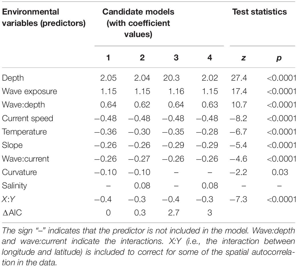
Table 1. The four selected candidate models explaining the kelp (Laminaria hyperborea) canopy abundance, i.e., the best model (model 1) and the three other models (model 2–4) considered to be almost equally good (ΔAIC < 4), the coefficient values for each environmental variable (predictor) included in each of the models, and the test statistics (z and p-values) for the predictors within the best model.

In CLM, a probability function is calculated for each response class, separately, and in R the default way of visualizing this is as accumulated curves added upon each other (shown for the best model selected in Supplementary Figure 2). However, to ease the interpretation of the results, we are isolating the probability of finding high abundance of kelp (i.e., dense kelp forest, class 3) and visualize this in a separate panel of figures based on the best model selected (Figures 2, 3). The probability of finding dense kelp forest increase from approximately 20% at low wave exposure, toward 100% in areas with high exposure (Figure 2). The probability of finding dense kelp forest is close to 100% in the shallowest areas but decreases to less than 10% around 30 m depth (Figure 2). Further, the effect of wave exposure seems to vary with depth (Figure 3A). Contrary to wave exposure, high current speed seems to have a negative impact on kelp abundance, i.e., the kelp forest gets more scattered as the current speed increases (Figure 2). The interaction between waves and currents shows that the two measures of water flow have opposite effects on kelp abundance (Figure 3B). The analysis indicates that the probability of finding dense kelp forests is larger at low temperatures (Figure 2). Kelp abundance also decreases with slope, i.e., as the terrain gets steeper, and is higher where the seafloor forms a basin or a relatively flat area (i.e., curvature values < 0) than at shoals.

Discussion

The main result of this study is that kelp abundance is modified by the combined impact of depth, waves and currents, and that dense kelp forests are found mainly in relatively shallow and flat terrain in wave exposed and low current areas. Kain (1971a) suggested that kelp responded differently to high currents and high wave exposures, and the studies of, e.g., Eckman et al. (2003) and Bekkby et al. (2014) on kelp morphology show that the impact of wave exposure and current speed are different. Our study confirms previous studies on the effects of wave exposure (e.g., Svendsen and Kain, 1971; Sjøtun and Fredriksen, 1995; Sjøtun et al., 1998; Gorman et al., 2012; Pedersen et al., 2012) and increases the relatively scarce knowledge on the effects of current speed and the interaction between these two water flow components (but see Bekkby et al., 2009, 2014, the discussion in Kain, 1971a and studies on other kelp species, e.g., Duggins et al., 2003; Eckman et al., 2003; Miller et al., 2011).

With the exception of the depth data, all the data on environmental conditions were modeled, using different methods and at different horizontal resolutions (from 25 to 800 m). This is a challenge for several reasons. First, there might be variation in water flow at spatial scales that is not captured by the models, but which has high impact on the abundance of kelp. An example is wave sheltering effects or increased ocean current levels due to shallows or other terrain structures not present in the models. As a result, the effect of smaller-scaled water flow, impacting nutrient uptake (Raven, 1981), lamina fouling (Strand and Weisner, 1996; Pihl et al., 1999) and wounding (de Bettignies et al., 2012), will not be detected by our analyses. Second, the models represent an overall level of water flow and more extreme events are not covered. Such extreme events, e.g., storm, might have a large impact on kelp abundance, kelp might be dislodged completely. Third, the algae themselves can change the water flow (e.g., Mork, 1996; Rosman et al., 2013), which is not taken into account in the wave exposure and ocean current models. However, having field measured environmental conditions at the scale (both in space and time) at which these data have been collected has not been possible, so using models has been our best option. And as our dataset is coarse classes of kelp abundance and a large spatial scale, we believe that our findings are reliable and shows large-scale relationships between kelp abundance and environmental conditions.

Effects of Wave Exposure and Ocean Current

Similar to other studies (Gorman et al., 2012; Smale et al., 2016) we find that high abundance of kelp occurs mainly in moderately exposed and exposed areas, and that kelp abundance decreases down to a single or few kelps per m² in very wave sheltered areas. The lack of L. hyperborea kelp in wave sheltered areas is most likely because it is outcompeted by the Saccharina latissima kelp (Kain, 1962). As the wave exposure increase, waves are moving of algal fronds, which maximizes the influx of light on the lamina and increases nutrient uptake by reducing the boundary diffusion layer (Gerard, 1982; Lobban and Harrison, 1994; Hurd et al., 1996). High wave exposure also keeps the lamina clean from epiphytic growth (Strand and Weisner, 1996; Pihl et al., 1999), ensuring high light influx which increases photosynthetic activity. We found no drop in abundance at high wave exposure levels, as L. hyperborea kelp is well adapted to high wave exposure and shows little damage or mortality after storms (Smale and Vance, 2015).

The impact of wave exposure on kelp abundance interacts with depth. This is probably related to large waves in exposed areas penetrating deeper compared to smaller waves in sheltered areas. Variation in wave exposure has little effect in the shallow areas, where kelp already occurs in high densities, and were the growth is not limited by light. In deeper areas, however, increases in wave exposure might move the algal fronds enough to have a positive impact on the light influx for light-limited kelps. In the deepest areas, where the waves no longer reach, the influence of increased wave exposure completely disappears.

We find that strong currents have a negative impact on kelp abundance. At low current speed there is a high probability of dense kelp forests. As the current speed increases, the kelp forest gets more scattered. Previously (Bekkby et al., 2014) we found that current speed has a positive effect on kelp properties, resulting in thicker stipes and bigger holdfasts. Our suggested explanation is that high currents impose problems with detachment or reduced settlement of kelp, creating low kelp abundance. However, the kelps that can persist in these high current speed areas, and thereby were sampled by Bekkby et al. (2014), are modified toward more strength-related characters, including morphological changes in the blade (as found by, e.g., Armstrong, 1989; Koehl et al., 2008). This hypothesis might also explain the findings of Rinde et al. (2014) of enhanced recovery of kelp forests after sea urchin grazing only up to a certain current speed threshold, after which the probability of recovery decreased with increasing current speed.

The current speed interacts with wave exposure to influence kelp abundance, with opposite (non-synergistic) effects. In the wave sheltered parts of the coast, with L. hyperborea abundances already being low, variation in current speed has no detectable impact on kelp abundance. This was a surprise and suggests that the difference in the frequency, intensity and direction of these two physical stressor results in these two types of water flow having different roles when it comes to structuring the distribution of kelp. This is supported by Miller et al. (2011), who suggested that there is a stronger morphological adaptations to high wave actions (orbital) than to the more unidirectional currents. However, as wave exposure increases (increasing the probability of high kelp abundances), a negative effect occurs when the current level also increases. These results suggest that kelp in wave exposed areas tolerates relatively high current speed levels and are able to resist being dislodged by having large holdfasts, thick and strong stipes, and narrow and robust laminas (Svendsen and Kain, 1971; Sjøtun and Fredriksen, 1995; Bekkby et al., 2014). However, at some point the water flow induced stress imposed by the increased ocean currents just gets too much and the abundance drops. There is unfortunately no data in areas of both high wave exposure and high current speed (Figure 3B), and conclusion on the kelp abundance in this part of the environmental space must be drawn with care.

When discussing the relative importance of wave exposure and ocean currents, the huge difference in the resolution of these models has to be discussed. The strongest ocean currents are confined to archipelagos, fjords, narrow sounds and areas of high terrain variability with strong tidal forcing (Sætre, 2007). These is not captured by the coarse (800 m) horizontal resolution of the current speed model used in our analyses, which could possibly explain the relatively low importance of current speed compared to wave exposure.

The probability of finding dense kelp forests is higher in basins and flat areas than on shoals. We assume that the curvature most likely represents an effect of ocean currents at a smaller scale than what is possible to be captured by the coarse ocean current model. Current speed has a negative impact on kelp abundance and the negative effect of shoals can be explained by increased current speed levels on these shoals. The confidence interval for the influence of curvature on kelp abundance was quite high throughout most of the curvature gradient. This makes the true response of curvature on kelp abundance uncertain (Table 1). Another example of this uncertainty is that the best model seems to have high probability of finding both scarce and dense kelp forests in flat areas (Supplementary Figure 2).

Effects of Depth and Terrain

Depth was, as expected and found in other studies (Bekkby et al., 2009; Gorman et al., 2012), the most important variable for explaining kelp abundance. Kelp abundance decreases with depth and the deepest observation of dense kelp forests is at 31.8 m depth (single kelps were found at 33.5 m depth), which is comparable to findings in other studies (e.g., Kain and Jones, 1964; lower growth limit of approx. 30 m depth). Depth is a proxy for light reaching the seabed, which is well known to have profound impact on recruitment, growth, size, biomass and density of L. hyperborea (Kain, 1971b; Lobban and Harrison, 1994; Sjøtun and Fredriksen, 1995; Smale et al., 2016). In our model, depth explains kelp abundance better than modeled light. This is most likely because depth is measured in the field, and is therefore relatively precise in space, while modeled light is based on a combination of low-resolution satellite models (250 m horizontal resolution) and a depth model with a 25 m horizontal resolution.

The probability of dense kelp forests decreases as the terrain gets steeper, which was also found by Kain (1971a), most likely because kelps have difficulties to attach to the seabed when it is very steep. The confidence interval of this response is largest at the steep end of the slope gradient, which reflects the small numbers of data collected in this environmental space.

Effects of Temperature

The study indicates that the probability of finding dense kelp forests is higher at low than at high temperatures. This was not expected, as the temperature values, as modeled, range from 5.8 to 9.3°C, which is within the temperature tolerance range (Bolton and Lüning, 1982). Even though the occurrence of kelp has previously been found to be correlated with temperature, the relationship has varied between seasons (Assis et al., 2016). Within the temperature range found in our dataset, which is based on a model being coarse both in space (800 m horizontal resolution) and time (January–August mean values), it is not expected that temperature should explain any of the variation found in the dataset. However, these mean values might be correlated with more extreme heat events in such a way that the high average temperature values we have in our models are found in areas that also have more extreme temperature during heat events. It is also important to note that the temperature in our study is negatively correlated with salinity (−0.72 when looking at mean values, Supplementary Figure 1), which indicates that we have an inner-outer gradient (from inner, freshwater influenced fjords to offshore, more saline coastal waters). Temperature also correlates (positively) to a certain degree with longitude (0.47), which also is an indication of an inner-outer relationship. Temperature correlates (negatively) to a certain degree with latitude (−0.46), which is an effect of the north-south gradient. As the density of both recruits, understory kelp and canopy kelp has been found to decrease with latitude (Rinde and Sjøtun, 2005), the effect of temperature might be confounded by the effect of latitude. It is worth noting that even though the abundance of kelp decreases with temperature, the probability of finding high kelp abundance is still higher than any of the other abundance classes (Supplementary Figure 2). The confidence interval is large at the low and high end of the temperature gradient (Figure 2), which reflects the small number of data collected and the uncertainty associated with this predictor.

Data Availability

The datasets generated for this study are available on request to the corresponding author.

Author Contributions

TB, ER, and HS planned the sampling of the data. TB, ER, HS, LT, JG, and HC did sampling of the data in the field since the very beginning of the National Program for Mapping of Biodiversity – Coast. JA modeled the ocean currents, temperature and salinity, and contributed to the interpretation of the water flow related results. TB, ER, HG, and SF contributed to the statistical analyses of the data, together with CS, who done her Master degree on these data. TB, HG, and SF supervised SM during her Master thesis work. All authors listed have contributed to the interpretation of the results and the writing of the manuscript.

Funding

This work was supported by the Ministry of Climate and Environment and the Ministry of Trade, Industry and Fisheries through the National Program for Mapping of Biodiversity – Coast.

Conflict of Interest Statement

The authors declare that the research was conducted in the absence of any commercial or financial relationships that could be construed as a potential conflict of interest.

Acknowledgments

We thank all the people along the coast who have hosted and assisted us in the field for more than a decade. We also thank the staff at the NIVA research infrastructure section for technical support, and Jan-Erik Thrane (NIVA), Jan Heuschele and Prof. Tom Andersen (both University of Oslo, Norway) for help with R programming.

Supplementary Material

The Supplementary Material for this article can be found online at: https://www.frontiersin.org/articles/10.3389/fmars.2019.00475/full#supplementary-material

Footnotes

1. ^ http://www.myroms.org

References

Abdullah, M. I., and Fredriksen, S. (2004). Production, respiration and exudation of dissolved organic matter by the kelp Laminaria hyperborea along the west coast of Norway. J. Mar. Biol. Assoc. UK 84, 887–894. doi: 10.1017/S002531540401015Xh
Albretsen, J., Sperrevik, A. K., Staalstrøm, A., Sandvik, A. D., Vikebø, F., and Asplin, L. (2011). NorKyst-800 Report No. 1 - User Manual and Technical Descriptions. Fisken & Havet, 2. Bergen: Institute of Marine Research.
Armstrong, S. L. (1989). The behavior in flow of the morphologically variable seaweed Hedophyllum sessile (C. Agardh) Setchell. Hydrobiology 183, 115–122. doi: 10.1007/BF00018716
Assis, J., Lucas, A. V., Bárbara, I., and Serrão, E. Á (2016). Future climate change is predicted to shift long-term persistence zones in the cold-temperate kelp Laminaria hyperborea. Mar. Environ. Res. 113, 174–182. doi: 10.1016/j.marenvres.2015.11.005
Bartón, K. (2018). MuMIn: Multi-Model Inference. R package version 1.40.4.Google Scholar
Bartsch, I., Wiencke, C., Bischof, K., Buchholz, C. M., Buck, B. H., Eggert, A., et al. (2008). The genus Laminaria sensu lato: recent insights and developments. Eur. J. Phycol. 43, 1–86. doi: 10.1080/09670260701711376
Bekkby, T., Angeltveit, G., Gundersen, H., Tveiten, L., and Norderhaug, K. M. (2015). Red sea urchins (Echinus esculentus) and water flow influence epiphytic macroalgae density. Mar. Biol. Res. 11, 375–384. doi: 10.1080/17451000.2014.943239
Bekkby, T., Bodvin, T., Bøe, R., Moy, F. E., Olsen, H., and Rinde, E. (2011). National Program for Mapping and Monitoring of Marine Biodiversity in Norway. Final Report for the Period 2007-2010. NIVA Report. 6105-2011. Fornebu: Norwegian, 31.
Bekkby, T., Rinde, E., Erikstad, L., and Bakkestuen, V. (2009). Spatial predictive distribution modelling of the kelp species Laminaria hyperborea. ICES J. Mar. Sci. 66, 2106–2115. doi: 10.1093/icesjms/fsp195
Bekkby, T., Rinde, E., Gundersen, H., Norderhaug, K. M., Gitmark, J., and Christie, H. (2014). Length, strength and water flow - the relative importance of wave and current exposure on kelp Laminaria hyperborea morphology. Mar. Ecol. Progr. Ser. 506, 61–70. doi: 10.3354/meps10778
Bolton, L. L., and Lüning, K. (1982). Optimal growth and maximal survival temperatures of Atlantic Laminaria species (Phaeophyta) in culture. Mar. Biol. 66, 89–94. doi: 10.1007/BF00397259
Burnham, K. P., and Anderson, D. R. (2002). Model Selection and Multimodel Inference. A Practical Information-Theoretic Approach. New York, NY: Springer.
Burnham, K. P., Anderson, D. R., and Huyvaert, K. (2011). AIC-model selection and multimodel inference in behavior ecology: some background observations and comparisons. Behav. Ecol. Sociobiol. 65, 23–35. doi: 10.1007/s00265-010-1084-z
Christensen, R. H. (2015). Ordinal - Regression Models for Ordinal Data. R package version 2015.6-28.Google Scholar
Davies, C. E., Moss, D., and Hill, M. O. (2004). EUNIS Habitat Classification Revised. European Topic Centre on Nature Protection and Biodiversity. Available at: https://eunis.eea.europa.eu/references/1473 (accessed July 19, 2019).
de Bettignies, T., Thomson, M. S., and Wernberg, T. (2012). Wounded kelps: patterns and susceptibility to breakage. Aquat. Biol. 17, 223–233. doi: 10.3354/ab00471
Duggins, D. O., Eckman, J. E., Siddon, C. E., and Klinger, T. (2003). Population, morphometric and biomechanical studies of three understory kelps along a hydrodynamic gradient. Mar. Ecol. Progr. Ser. 265, 57–76. doi: 10.3354/meps265057
Eckman, J., Siddon, C., and Klinger, T. (2003). Population, morphometric and biomechanical studies of three understory kelps along a hydrodynamic gradient. Mar. Ecol. Progr. Ser. 265, 57–76. doi: 10.3354/meps265057
Egbert, G. D., and Erofeeva, S. Y. (2002). Efficient inverse modeling of barotropic ocean tides. J. Atmos. Oceanic Technol. 19, 183–204.
Eriksson, B. K., Sandström, A., Isæus, M., Schreiber, H., and Karås, P. (2004). Effects of boating activities on aquatic vegetation in the Stockholm Archipelago, Baltic Sea. Estuar. Coast. Shelf Sci. 61, 339–349. doi: 10.1016/j.ecss.2004.05.009
Gerard, V. A. (1982). In situ water motion and nutrient uptake by the giant kelp Macrocystis pyrifera. Mar. Biol. 69, 51–54. doi: 10.1007/BF00396960
Gorman, D., Bajjouk, T., Populus, J., Vasquez, M., and Ehrhold, A. (2012). Modeling kelp forest distribution and biomass along temperate rocky coastlines. Mar. Biol. 160:309325. doi: 10.1007/s00227-013-2203-y
Gundersen, H., Bryan, T., Chen, W., Moy, F. E., Sandman, A. N., Sundblad, G., et al. (2016). Ecosystem Services in the Coastal Zone of the Nordic Countries. Copenhagen: Nordic Council of Ministers.
Haidvogel, D. B., Arango, H., Budgell, W. P., Cornuelle, B. D., Curchitser, E., Di Lorenzo, E., et al. (2008). Ocean forecasting in terrain-followingcoordinates: formulation and skill assessment of the regional ocean modeling system. J. Comp. Phys. 227, 3595–3624. doi: 10.1016/j.jcp.2007.06.016
Hurd, C. L., Harrison, P. J., and Druehl, L. D. (1996). Effect of seawater velocity on inorganic nitrogen uptake by morphologically distinct forms of Macrocystis integrifolia from wave-sheltered and exposed sites. Mar. Biol. 126, 205–214. doi: 10.1007/BF00347445
Isæus, M. (2004). Factors Structuring Fucus Communities at Open and Complex Coastlines in the Baltic Sea. PhD Thesis. Stockholm University: Stockholm.
Isæus, M., and Rygg, B. (2005). Wave exposure calculations for the Finnish coast. NIVA Rep. 5075:24.
Kain, J. M. (1962). Aspects Of the biology of Laminaria hyperborea I. Vertical distribution. J. Mar. Biol. Assoc. UK 42, 377–385. doi: 10.1017/S0025315400001363
Kain, J. M. (1971b). The biology of Laminaria hyperborea. VI. Some Norwegian populations. J. Mar. Biol. Assoc. UK 51, 387–408. doi: 10.1017/S0025315400031866
Kain, J. M., and Jones, N. S. (1964). Aspects of the biology of Laminaria hyperborea III. Survival and growth of gametophytes. J. Mar. Biol. Assoc. UK 44, 415–433. doi: 10.1017/S0025315400024929
Koehl, M. A. R., Silk, W. K., Liang, H., and Mahadevan, L. (2008). How kelp produce blade shapes suited to different flow regimes: a new wrinkle. Int. Comp. Biol. 48, 834–851. doi: 10.1093/icb/icn069
Legendre, P. (1993). Spatial autocorrelation: trouble or new paradigm? Ecology 74, 1659–1673. doi: 10.2307/1939924
Lobban, C. S., and Harrison, P. J. (1994). Seaweed Ecology and Physiology. Cambridge: Cambridge University Press.
Miller, S. M., Hurd, C. L., and Wing, S. R. (2011). Variations in growth, erosion, productivity, and morphology of Ecklonia radiata (Alariaceae; Laminariales) along a fjord in southern New Zealand. J. Phycol. 47, 505–516. doi: 10.1111/j.1529-8817.2011.00966.x
Mork, M. (1996). The effect of kelp in wave dampening. Sarsia 80, 323–327. doi: 10.1080/00364827.1996.10413607
Norderhaug, K. M., and Christie, H. (2009). Sea urchin grazing and kelp re-vegetation in the NE Atlantic. Mar. Biol. Res. 5, 515–528. doi: 10.1080/17451000902932985
Norderhaug, K. M., Christie, H., Fosså, J. H., and Fredriksen, S. (2005). Fish–macrofauna interactions in a kelp (Laminaria hyperborea) forest. J. Mar. Biol. Assoc. UK 85, 1279–1286. doi: 10.1017/S0025315405012439
Norderhaug, K. M., Christie, H., Rinde, E., Gundersen, H., and Bekkby, T. (2014). Importance of wave and current exposure to fauna communities in Laminaria hyperborea kelp forests. Mar. Ecol. Progr. Ser. 502, 295–301. doi: 10.3354/meps10754
Økland, R. H., Rydgren, K., and Økland, T. (2003). Plant species composition of boreal spruce swamp forests: closed doors and windows of opportunity. Ecology 84, 1909–1919. doi: 10.1890/0012-9658(2003)084%5B1909:pscobs%5D2.0.co;2
Pedersen, M. F., Nejrup, L. B., Fredriksen, S., Christie, H., and Norderhaug, K. M. (2012). Effects of wave exposure on population structure, demography, biomass and productivity in kelp Laminaria hyperborea. Mar. Ecol. Progr. Ser. 451, 45–60. doi: 10.3354/meps09594
Pihl, L., Svenson, A., Moksnes, P. O., and Wennehage, H. (1999). Distribution of green algal mats throughout shallow soft bottoms of the Swedish Skagerrak archipelago in relation to nutrient sources and wave exposure. J. Sea Res. 41, 281–295. doi: 10.1016/S1385-1101(99)00004-0
Populus, J., Vasquez, M., Albrecht, J., Manca, E., Agnesi, S., Al Hamdani, Z., et al. (2017). EUSeaMap. A European Broad-Scale Seabed Habitat Map. (Plouzané: Ifremer), 174. doi: 10.13155/49975
R Development Core Team (2017). R: A Language and Environment for Statistical Computing. Vienna: R Foundation for Statistical Computing.
Raven, J. A. (1981). Nutritional strategies of submerged benthic plants: the acquisition of C, N and P by rhizophytes and haptophytes. New Phytol. 88, 1–30. doi: 10.1111/j.1469-8137.1981.tb04564.x
Rinde, E., Christie, H., Fagerli, C. W., Bekkby, T., Gundersen, H., Norderhaug, K. M., et al. (2014). The influence of physical factors on kelp and sea urchin distribution in previously and still grazed areas in the NE Atlantic. PLoS One 9:e0100222. doi: 10.1371/journal.pone.0100222
Rinde, E., Rygg, B., Bekkby, T., Isæus, M., Erikstad, L., Sloreid, S.-E., et al. (2006). Documentation of Marine Nature Type Models Included in Directorate of Nature Management’s DATABASE NATURBASE. First Generation Models for the Municipalities Mapping of Marine Biodiversity 2007. NIVA Report. 5321. Fornebu: Norwegian.
Rinde, E., and Sjøtun, K. (2005). Demographic variation in the kelp Laminaria hyperborea along a latitudinal gradient. Mar. Biol. 146, 1051–1062. doi: 10.1007/s00227-004-1513-5
Rosman, J. H., Denny, M. W., Zeller, R. N., Monismith, S. G., and Koseff, J. E. (2013). Interaction of waves and currents with kelp forests (Macrocystis pyrifera): insights from a dynamically scaled laboratory model. Limnol. Oceanogr. 58, 790–802. doi: 10.4319/lo.2013.58.3.0790
Saulquin, B., Hamdi, A., Gohin, F., Populus, J., Mangin, A., and d’Andon, O. F. (2013). Estimation of the diffuse attenuation coefficient KdPAR using MERIS and application to seabed habitat mapping. Rem. Sens. Environ. 128, 224–233. doi: 10.1016/j.rse.2012.10.002
Schoschina, E. V. (1997). On Laminaria hyperborea (Laminariales, phaeophyceae) on the Murman coast of the Barents Sea. Sarsia 82, 371–373. doi: 10.1080/00364827.1997.10413663
Shchepetkin, A. F., and McWilliams, J. C. (2005). The regional ocean modeling system (ROMS): a split-explicit, free-surface, topography-following coordinates ocean model. Ocean Model. 9, 347–404. doi: 10.1016/j.ocemod.2004.08.002
Sjøtun, K., and Fredriksen, S. (1995). Growth allocation in Laminaria hyperborea (Laminariales, Phaeophyceae) in relation to age and wave exposure. Mar. Ecol. Progr. Ser. 126, 213–222. doi: 10.3354/meps126213
Sjøtun, K., Fredriksen, S., and Rueness, J. (1998). Effect of canopy biomass and wave exposure on growth in Laminaria hyperborea (Laminariaceae: Phaeophyta). Eur. J. Phycol. 33, 337–343. doi: 10.1080/09670269810001736833
Skamarock, W., Klemp, J., Dudhia, J., Gill, D., Barker, D., Duda, M., et al. (2008). A Description of the Advanced Research WRF Version 3. NCAR Technical Note NCAR/TN-475+STR. 113. Available at: www.mmm.ucar.edu/weather-research-and-forecasting-model (accessed July 19, 2019).
Smale, D., and Vance, T. (2015). Climate-driven shifts in species’ distributions may exacerbate the impacts of storm disturbances on North-east Atlantic kelp forests. Mar. Freshw. Res. 67, 65–74. doi: 10.1071/MF14155
Smale, D. A., Burrows, M., Evans, A., King, N., Sayer, M., Yunnie, A., et al. (2016). Linking environmental variables with regional-scale variability in ecological structure and standing stock of carbon within UK kelp forests. Mar. Ecol. Progr. Ser. 542, 79–95. doi: 10.3354/meps11544
Strand, J. A., and Weisner, S. E. B. (1996). Wave exposure related growth of epiphyton: implications for the distribution of submerged macrophytes in eutrophic lakes. Hydrobiology 325, 113–119. doi: 10.1007/BF00028271
Svendsen, P., and Kain, J. M. (1971). The taxonomic status, distribution, and morphology of Laminaria cucullata sensu Jorde and Klavestad. Sarsia 46, 1–22. doi: 10.1080/00364827.1971.10411185
Sætre, R. (2007). The Norwegian Coastal Current: Oceanography and Climate. Norway: Tapir Academic Press, 159.
Wei, T., and Simko, V. (2017). R package «corrplot»: Visualization of a Correlation Matrix (Version 0.84). Available at: https://github.com/taiyun/corrplot (accessed July 19, 2019).
Whittick, A. (1983). Spatial and temporal distributions of dominant epiphytes on the stipes of Laminaria hyperborea (Gunn.) Fosl. (Phaeophyta: Laminariales) in S.E. Scotland. J. Exp. Mar. Biol. Ecol. 73, 1–10. doi: 10.1016/0022-0981(83)90002-3
Keywords: Laminaria hyperborea, macroalgae, water flow, wave exposure, current speed, environmental variables, Norway
Citation: Bekkby T, Smit C, Gundersen H, Rinde E, Steen H, Tveiten L, Gitmark JK, Fredriksen S, Albretsen J and Christie H (2019) The Abundance of Kelp Is Modified by the Combined Impact of Depth, Waves and Currents. Front. Mar. Sci. 6:475. doi: 10.3389/fmars.2019.00475
Received: 02 May 2019; Accepted: 15 July 2019;
Published: 06 August 2019.
Edited by:
Libin Zhang, Institute of Oceanology (CAS), ChinaReviewed by:
Bela H. Buck, Alfred Wegener Institute Helmholtz Centre for Polar and Marine Research (AWI), GermanyYukio Agatsuma, Tohoku University, Japan
Huang Wei, State Oceanic Administration, China
Copyright © 2019 Bekkby, Smit, Gundersen, Rinde, Steen, Tveiten, Gitmark, Fredriksen, Albretsen and Christie. This is an open-access article distributed under the terms of the Creative Commons Attribution License (CC BY). The use, distribution or reproduction in other forums is permitted, provided the original author(s) and the copyright owner(s) are credited and that the original publication in this journal is cited, in accordance with accepted academic practice. No use, distribution or reproduction is permitted which does not comply with these terms.
*Correspondence: Trine Bekkby, trine.bekkby@niva.no