Surface Ocean Dispersion Observations From the Ship-Tethered Aerostat Remote Sensing System
 Daniel F. Carlson1,2*
  Tamay Özgökmen3
  Guillaume Novelli3 Cedric Guigand3
  Henry Chang4
  Baylor Fox-Kemper5
  Jean Mensa6,7 Sanchit Mehta3 Erick Fredj8
  Helga Huntley4
  A. D. Kirwan Jr.4
  Maristella Berta9 Mike Rebozo3
  Milan Curcic10
  Ed Ryan3 Björn Lund11 Brian Haus3 Jeroen Molemaker12
  Cameron Hunt13† Shuyi Chen10
  Laura Bracken3
  Jochen Horstmann14
- 1Department of Earth, Ocean and Atmospheric Science, Florida State University, Tallahassee, FL, United States
- 2Department of Bioscience, Arctic Research Centre, Aarhus University, Aarhus, Denmark
- 3Rosentiel School for Marine and Atmospheric Science, University of Miami, Miami, FL, United States
- 4School of Marine Science and Policy, University of Delaware, Newark, DE, United States
- 5Department of Earth, Environmental and Planetary Science, Brown University, Providence, RI, United States
- 6Department of Geology and Geophysics, Yale University, New Haven, CT, United States
- 7Risk Management Solutions, London, United Kingdom
- 8Department of Computer Science, Jerusalem Institute of Technology, Jerusalem, Israel
- 9Consiglio Nazionale delle Ricerche, Istituto di Scienze Marine, La Spezia, Italy
- 10Department of Atmospheric Sciences, University of Washington, Seattle, WA, United States
- 11Center for Southeastern Tropical Advanced Remote Sensing, University of Miami, Miami, FL, United States
- 12Institute of Geophysics and Planetary Physics, University of California, Los Angeles, Los Angeles, CA, United States
- 13Doolittle Institute, Tampa, FL, United States
- 14Department of Radar Hydrography, Helmholtz Zentrum Geesthacht, Geesthacht, Germany
Oil slicks and sheens reside at the air-sea interface, a region of the ocean that is notoriously difficult to measure. Little is known about the velocity field at the sea surface in general, making predictions of oil dispersal difficult. The Ship-Tethered Aerostat Remote Sensing System (STARSS) was developed to measure Lagrangian velocities at the air-sea interface by tracking the transport and dispersion of bamboo dinner plates in the field of view of a high-resolution aerial imaging system. The camera had a field of view of approximately 300 × 200 m and images were obtained every 15 s over periods of up to 3 h. A series of experiments were conducted in the northern Gulf of Mexico in January-February 2016. STARSS was equipped with a GPS and inertial navigation system (INS) that was used to directly georectify the aerial images. A relative rectification technique was developed that translates and rotates the plates to minimize their total movement from one frame to the next. Rectified plate positions were used to quantify scale-dependent dispersion by computing relative dispersion, relative diffusivity, and velocity structure functions. STARSS was part of a nested observational framework, which included deployments of large numbers of GPS-tracked surface drifters from two ships, in situ ocean measurements, X-band radar observations of surface currents, and synoptic maps of sea surface temperature from a manned aircraft. Here we describe the STARSS system and image analysis techniques, and present results from an experiment that was conducted on a density front that was approximately 130 km offshore. These observations are the first of their kind and the methodology presented here can be adopted into existing and planned oceanographic campaigns to improve our understanding of small-scale and high-frequency variability at the air-sea interface and to provide much-needed benchmarks for numerical simulations.
1. Introduction
In April 2010, the explosion of the Deepwater Horizon (DwH) oil platform in the DeSoto Canyon of the Gulf of Mexico (GoM) resulted in the largest accidental marine oil spill in history (Crone and Tolstoy, 2010). In the aftermath, a great need for transport and dispersion forecasts at the air-sea interface over a large range of spatial (100s of m to 100s of km) and temporal (hours to months) scales became clear (Liu et al., 2011; Mariano et al., 2011). Hydrocarbons were present in a range of environments, from the open ocean to the shoreline, complicating the problem of predicting their motion. Putting aside the complexities of the fate of hydrocarbons in water specifically, even the prediction of the transport of near-surface water masses over such a range of scales and environments has been impeded by a lack of observations of scale-dependent dispersion that span the relevant spatio-temporal scales (Poje et al., 2014). While recent observational campaigns have been devoted to submesoscale transport and mixing (Schroeder et al., 2012; Poje et al., 2014; Berta et al., 2015; Coelho et al., 2015; Shcherbina et al., 2015; Ohlmann et al., 2017; Pascual et al., 2017; Petrenko et al., 2017), relatively few in situ studies (e.g., Miyao and Isobe, 2016; Matsuzaki and Fujita, 2017) have quantified near-surface velocities at oceanic boundary layer scales (seconds to hours and meters to 100 s of m).
Traditional ocean observation tools (e.g., drifters, ships, and satellites) are limited in their ability to both measure velocities at the air-sea interface, where slicks and sheens of oil reside, and to resolve dispersion at oceanic boundary layer scales. The drifter trajectory data collected during the Grand Lagrangian Deployment (GLAD) in 2012 was successful in improving velocity estimates (Berta et al., 2015; Coelho et al., 2015), data-assimilating models (Carrier et al., 2014; Jacobs et al., 2014), and understanding of turbulence through dispersion statistics (Poje et al., 2014, 2017). However, due to uncertainties in GPS positioning of the drifters (Haza et al., 2014) and the initial drifter separation distances, this technology was capable of accurately sampling only the larger submesoscale and mesoscale features. Haza et al. (2014) report that statistics on scales 20–60 times larger than the 5 m GPS position uncertainty may be contaminated (i.e., 100–300 m).
Recent developments in modeling and theory have emphasized the importance of the connections between submesoscale fronts, filaments, and eddies and the more isotropic scales of traditional boundary layer turbulence (Taylor and Ferrari, 2009; Hamlington et al., 2014; McWilliams et al., 2015; Smith et al., 2016; Suzuki et al., 2016; McWilliams, 2017). The smallest scales of the submesoscale are also of great interest, because it is on these scales where nonhydrostatic turbulent effects first become important, which dynamically delineates the beginnings of the three-dimensional turbulence that is smaller than the submesoscale (Mahadevan and Tandon, 2006; Hamlington et al., 2014; Haney et al., 2015; Mensa et al., 2015; Suzuki and Fox-Kemper, 2016). Large Eddy Simulations (LES) show that intense localized submesoscale restratification occurs intermittently on these scales in competition with mixing by three-dimensional turbulence when forced with winds, waves, and/or convective cooling (Mahadevan et al., 2010; Smith et al., 2016; Bachman et al., 2017; Whitt and Taylor, 2017), but observations of this regime are rare and challenging in general and are particularly relevant to the study of the dispersion of buoyant substances like oil. These interactions between boundary layer turbulence, surface forcing, and submesoscale restratification are not captured in the standard submesoscale parameterizations (Fox-Kemper et al., 2008, 2011; Bachman et al., 2017; Whitt and Taylor, 2017; Callies and Ferrari, 2018). Their effects on near-surface dispersion are therefore also missing from regional models needed to capture larger submesoscale and mesoscale phenomena (Haza et al., 2014; Mensa et al., 2015).
Boundary layer turbulence observations are common from many platforms: the Floating Instrument Platform (FLIP; Sutherland and Melville, 2015), Lagrangian floats (e.g., D'Asaro et al., 2014), microstructure profilers (e.g., Sutherland et al., 2014), and moorings (e.g., Prytherch et al., 2013). However, they have not been connected, conceptually or technologically, to the larger scales observed by surface drifters. To fill this observational gap, the classic tools of messages in bottles (e.g., Williams et al., 1977) and drift cards (e.g., Yeske and Green, 1975) were brought into the modern era: Continuous quantitative visual monitoring, as in the famous parsnip experiments of Richardson and Stommel (1948), of buoyant and biodegradable bamboo dinner plates from a ship-tethered aerostat equipped with a high-resolution camera and positioning system.
Section 2.1 and Table 1 outline the minimum operating requirements for observations of Lagrangian transport at the air-sea interface in the open ocean that resolve the spatiotemporal scales relevant to oceanic boundary layer turbulence. We argue that a low-altitude aerial remote sensing platform satisfies these requirements and section 2.2 describes the ship-tethered aerostat remote sensing system (STARSS) and its deployment during the Lagrangian submesoscale experiment (LASER). Supporting datasets from the LASER experiment are briefly described in section 2.3. Image analysis techniques are presented in section 2.4. Results from a STARSS experiment at an offshore density front in the northern Gulf of Mexico are presented in section 3 and discussed in section 4. The performance of STARSS is assessed in the discussion and improvements to the system are suggested.
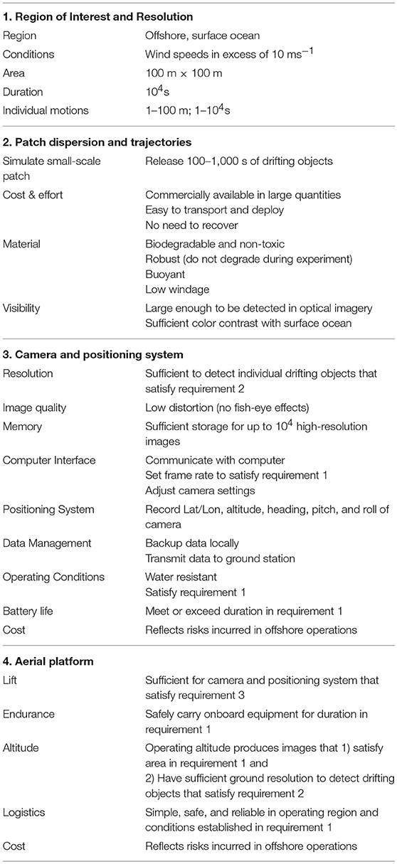
Table 1. Design requirements.
2. Methods
2.1. Design Requirements
Observations of Lagrangian transport and dispersion on the surface of the ocean at the spatiotemporal scales relevant to oceanic boundary layer turbulence present a unique challenge, especially in an offshore environment. To understand the transport and evolution of the patches and filaments of oil observed during the Deepwater Horizon spill (see, e.g., Figure 5a in Lumpkin et al., 2017), an observing system must be able to monitor an area of the surface ocean that is approximately O(100 × 100 m) while also resolving motions over spatial and temporal scales of O(1–100 m) and O(1–104s), respectively (see Table 1).
Existing oceanographic instrumentation and techniques could not satisfy these operational requirements in an open ocean setting. Land-based observing systems that are typically used to produce maps of surface currents, like high frequency (HF) radar (e.g., Carlson et al., 2010), cannot resolve the spatial and temporal scales of interest at distances that exceed 100 km from land. Similarly, satellite remote sensing has sufficient spatial and temporal resolution to investigate submesoscale dynamics (Qazi et al., 2014; Vanhellemont and Ruddick, 2014; Delandmeter et al., 2017; Marmorino et al., 2017; Rascle et al., 2017) but currently lacks the necessary temporal resolution to track dispersion due to boundary layer turbulence. Frequent cloud cover is an additional limitation imposed on passive satellite imagery. Marine x-band radar can also be processed to estimate surface currents but the spatial and temporal binning required to reduce uncertainties means that the smaller spatiotemporal scales of interest are not resolved (see section 2.3.4 and references therein).
Trajectories of particles that are advected by the velocity field are sometimes easier to observe than the full flow field itself (Salazar and Collins, 2009). Surface drifters are commonly used for this purpose, but standard GPS accuracy is insufficient to resolve the smaller spatial scales of interest here (Haza et al., 2014). Differential GPS (DGPS) and real-time kinematic (RTK) GPS (Suara et al., 2015) can produce position estimates with accuracies O(10 cm) and O(1 cm), respectively, but accuracy degrades with distance from base station measurements. Furthermore, most DGPS and RTK GPS sensors typically log positions internally, requiring each unit to be retrieved to download data, which complicates field logistics.
Recently, Matsuzaki and Fujita (2017) and Miyao and Isobe (2016) used a balloon to track objects in optical imagery. A similar system capable of tracking many (100 s–1,000) objects drifting on the surface of the ocean over periods of seconds to hours could be used. The use of drifting objects introduces additional design requirements that relate both to the properties of the objects and the capabilities of the aerial imaging system. The drifting objects must be readily available in large numbers, low-cost, biodegradable, subject to minimal windage, and detectable in aerial imagery (see Table 1). Historically, drift cards, or computer punch cards, and bottles have been used to study surface Lagrangian transport for well over a century (Garstang, 1898). In the past, drift cards typically provided only information about initial and final locations (e.g., Williams et al., 1977; Levin, 1983), though in rare cases they have been used to quantify short-term transport (Yeske and Green, 1975).
Computer punch cards have not been used for decades so other products were evaluated, including cardboard pizza boxes, plywood, and bamboo dinner plates. These materials were subjected to tests in the SUrge STructure Atmospheric INteraction (SUSTAIN) facility and in coastal waters near the Rosenstiel School for Marine and Atmospheric Sciences (RSMAS) of the University of Miami. The bamboo plates produced the most promising results as they did not degrade quickly, like cardboard, and were easily and cheaply available for purchase in large quantities, non-toxic, and biodegradable. The bamboo plates were 2 mm thick and had a draft of 1.75 cm and floated in the upper few cm of the water column for periods in excess of 6 h without a change in buoyancy or loss of structural integrity. Following the successful deployment of bamboo plates for STARSS, they have been adopted for drone-based observations near the mouth of the Mississippi River (Laxague et al., 2018). The plates were 28 cm in diameter and their natural color provided sufficient contrast with surface ocean waters in test images. A subset of the plates were painted with natural, non-toxic paint by students in Miami-area schools as part of an outreach program by the Consortium for Advanced Research on Transport of Hydrocarbon in the Environment (CARTHE; http://carthe.org) and to test whether such color differentiation could help in the linking step of the trajectory reconstruction (see section 2.4.4).
Imaging system requirements are summarized in Table 1. One of the main requirements was the ability to resolve individual bamboo plates. Cost, power consumption, weight, memory, and field of view (FOV) were also taken into account when evaluating cameras and lenses. Additionally, the horizontal and vertical position of the camera, as well as its orientation (pitch, roll, and heading), must also be recorded to georectify the imagery (see section 2.4.2).
The primary considerations for the aerial platform were endurance, reliability, ease of use, and cost (see Table 1). There are many platforms available for aerial imaging and there are several ‘turn-key’ commercial options available for monitoring. The requirement list eliminated manned aircraft, unmanned aerial systems (UAS), and most turn-key commercial options. Manned aircraft flights are expensive, especially considering the transit time to the offshore experiment location. Additionally, manned aircraft are better suited for synoptic mapping of surface ocean properties, like sea surface temperature (SST; see section 2.3.5). UAS have become important tools in oceanographic research (Whitehead and Hugenholtz, 2014; Whitehead et al., 2014; Brouwer et al., 2015; Klemas, 2015; Reineman et al., 2016) and were initially considered during the planning stage. However, planning began in 2013 and LASER was carried out in January-February 2016, before the FAA simplified the regulations for non-recreational use of UAS. Most commercial monitoring systems used a tethered aerostat or balloon that carried an imaging system and other systems. Many commercial systems were evaluated and ultimately rejected due to the cost and/or the capabilities of the onboard imaging system.
The tethered aerostat was selected as an aerial platform for ease of regulatory compliance, persistence, high lift capacity, and stable flight characteristics. Tethered aerostats and balloons have a long history: They have been used as an aerial imaging and reconnaissance platform for over 100 years (Brewer, 1902; Crawford, 1924; Vierling et al., 2006) and have also seen extensive use in studies of the planetary boundary layer (see Vierling et al., 2006 for a review). Tethered aerostats and balloons have been used at sea and in coastal areas to provide situational awareness during oil spill exercises (Hansen, 2015; Jacobs et al., 2015), to study melt ponds on sea ice (Derksen et al., 1997), to measure toxin levels during in situ oil burning operations during the DwH spill (Aurell and Gullett, 2010), to study surf-zone dynamics (Bezerra et al., 1997), to quantify macro-debris on beaches (Nakashima et al., 2011) and on the sea surface (Kako et al., 2012), to monitor marine mammals (Flamm et al., 2000), to study shoreline changes (Eulie et al., 2013), and to track floating buoys on the surface of the ocean (Miyao and Isobe, 2016). While Miyao and Isobe (2016) and Kako et al. (2012) used a ship-tethered balloon to track drifting buoys and marine debris, respectively, their overall scientific goals and their methodology differed from those of LASER and STARSS. Specifically, Miyao and Isobe (2016) and Kako et al. (2012) used a blimp-style balloon that was only suitable for flights in light winds to track O(10) drifting objects.
Modern aerostats are equipped with a sail that keeps the nose of the envelope pointed into the wind and also causes tether tension to increase with wind speed. As a result, aerostats exhibit relatively stable flight characteristics even in wind speeds over 10 ms−1. Federal regulations governing aerostat flights are outlined in Part 101, subpart B of the Code of Federal Regulations (see http://www.ecfr.gov). In short these regulations permit flights that are conducted at least 8 km (5 miles) from any airport, at a maximum altitude of 150 m (500 ft), with a minimum clearance of 150 m below any cloud base, a minimum of 4.8 km (3 miles) visibility, and the use of an automatic emergency deflation device. No licenses or certifications are required for aerostat operators.
2.2. STARSS Development and Deployment
STARSS was equipped with a Canon EOS 5DSR Mk III 50.6 megapixel (8,688 × 5,792 pixels) digital single lens reflex (DSLR) camera that was paired with a Canon 17–40 mm lens. A battery grip was used to extend the battery life and two 512 GB memory cards were installed in the camera. An Inertial Labs GPS-aided inertial navigation system (INS) was mounted next to the camera with the intention of using the latitude, longitude, altitude, pitch, roll, and heading output by the INS to perform absolute, or direct, rectification (see section 2.4.2). The INS processed raw position and altitude measurements from a NovaTel global navigation satellite system (GNSS) antenna, pressure data, and accelerations and rotation rates from a micro-electrical-mechanical systems (MEMS) inertial motion unit (IMU) using Inertial Labs' proprietary extended Kalman filter (EKF). The total weight of the camera, lens, battery grip, INS, and data cables exceeded 2 kg, which prohibited the use of a gimbal for camera stabilization.
An Odroid-C1 single board computer (SBC) was used for camera control and data management. A Ubiquiti Networks 5 GHz WiFi bridge connected the STARSS onboard computer to the ground station computer and allowed images to be viewed in near-real-time. The SBC, WiFi bridge, and INS were powered by a 7 Ah, 24 V sealed lead acid battery pack and a custom power distribution board that was capable of powering the components for periods of approximately 4 hr. STARSS instruments are shown in Figure 1A. A Python script acquired images every 15 s though infrequent errors occasionally increased the time between successive images to 30–90 s and copied each new image to a 256 GB USB drive and to the ground station. Images were saved in three locations (camera memory card, USB drive, and ground station computer) to ensure preservation of data in the event of a system failure or a crash. The ground station operators could adjust shutter speed and aperture settings in the Python script using gphoto2 calls (http://www.gphoto.org/). Near-real-time imagery allowed the operators to keep STARSS in position over the patch of plates (Figure 1B).
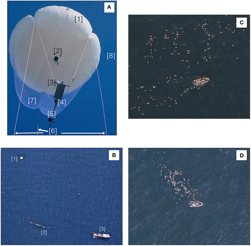
Figure 1. (A) STARSS consists of large aerostat (1), an emergency deflation device (2), a 5 GHz WiFi bridge (3), a NovaTel GNSS antenna (4), a 50.6 megapixel Canon 5DSR Mk III DSLR and INS (5), handling lines for launch and recovery (6), a sail (7), and a tether (8). The onboard computer and batteries were stored in a waterproof case on the top of the instrument frame (not visible). (B) An aerial image of a STARSS dispersion experiment. STARSS (1) is positioned over a patch of bamboo plates (2) and is tethered to the tender vessel (M/V Masco VIII; 3). (C) A grid deployment. (D) A patch deployment.
All components were mounted on an aluminum frame, with a combined weight of approximately 10 kg (Figure 1A). A safety factor of three, therefore, necessitated an aerostat with a lift capacity of 30 kg. STARSS was built around a large (4 m diameter, 38 m3), helium-filled Skydoc model 20 aerostat with a lift capacity of 30 kg (Figure 1A). The instrument frame was suspended from the aerostat's three control lines and an electric winch was used to control the ascent/descent and maximum altitude of the aerostat.
Ten STARSS dispersion experiments were conducted over five nonconsecutive days in late January and early February 2016. STARSS was flown from the M/V Masco VIII, an offshore supply vessel chartered by CARTHE for LASER (Figure 1). The geographic locations in which aerostat flights were permissible were limited by the large expanses of airspace that are dedicated to military training operations in the Gulf of Mexico. Offshore oil and gas installations in the region are serviced regularly by helicopters, which presented an additional logistical challenge. Therefore, STARSS flight operations during LASER were coordinated over a year in advance with the Federal Aviation Administration (FAA), who then alerted the Gulf Coast helicopter companies of our operations and facilitated a Notice to Airmen (NOTAM) for the LASER experiment period (Figure 2).
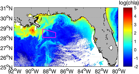
Figure 2. The Gulf of Mexico with the STARSS area of operation, as established by agreement with the Federal Aviation Administration and Gulf Coast Helicopter operators, outlined in magenta. A MODIS Aqua chlorophyll-a image that was acquired on 10 February 2016 reveals a feature-rich submesoscale environment in the area of interest.
A typical STARSS experiment consisted of inflation, launch, ascent to 150 m altitude, plate release, and image acquisition until the majority of the plates spread out of the FOV or were influenced by the ship. All flights were conducted during daylight hours. Plates were either released from the M/V Masco VIII or from a small workboat launched from the R/V Walton Smith. Two plate deployment patterns were employed: a dense, small patch and a grid-like array (Figures 1C,D). The advantage of patch deployments is the short deployment time. However, the proximity and occasional overlap of plates complicate particle tracking. Therefore, patch releases are more amenable to cloud dispersion analysis (e.g., Okubo, 1971), whereas the gridded deployments permit more detailed quantitative analysis based on particle tracking velocimetry (PTV, see section 2.4.4) but require coordination between STARSS operators and the small boat crew.
The focal length of the lens was kept constant during each experiment, but different focal lengths were used and were set by taping the lens in place. Focal lengths of 17, 21, and 23 mm were used. At an altitude of 150 m, a focal length of 17 mm resulted in a nadir-looking FOV of 318 × 235 m while the 23 mm focal length resulted in a FOV of 212 × 157 m. At 150 m, focal lengths of 17 and 23 mm resulted in nadir-looking ground resolutions of 3.67 and 2.7 cm / pixel, which was adequate to resolve the 28 cm diameter bamboo plates. Table 2 summarizes these parameters.
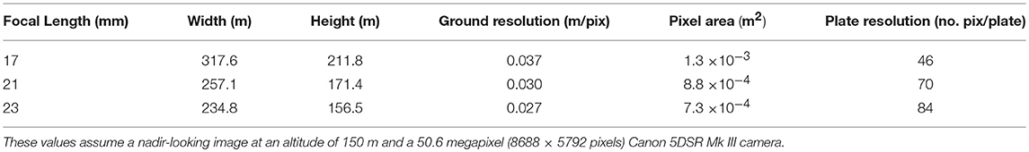
Table 2. Image dimensions, ground resolution, pixel area, and the number of pixels per 28 cm diameter bamboo plate are presented for the focal lengths used during the LASER experiment.
2.3. Supporting Data
LASER was carried out by in the northern GoM in January-February 2016 (Figure 2). One of the goals of the LASER experiment was connecting the oceanic boundary layer scales to the smaller scales of the submesoscale (section 2.3.1) using the STARSS and surface drifter observations. An unprecedented combination of observational data provide context for STARSS observations and these supporting data are briefly summarized here.
2.3.1. Drifter Deployments
Approximately 1,000 biodegradable surface drifters (Novelli et al., 2017) were deployed during LASER (D'Asaro et al., 2018). The drifters consisted of a donut-shaped float with the battery and electronics housing in the center, connected to a four-panel drogue. Drogued drifters were shown to follow the integrated currents of the top 60 cm of the water column under a wide range of conditions (Novelli et al., 2017). Drifters without drogues were also observed during LASER (Haza et al., 2018); these generally follow the upper 5 cm of flow but are subject to Stokes drift and increased windage. The drifters extend the observational range of scale-dependent dispersion to the submesoscale.
2.3.2. Meteorology and Vessel Motion
Wind speed, air temperature, and relative humidity were measured on the M/V Masco VIII at 10 Hz. Quality control measures eliminated data that (1) experienced a change in heading >40°, (2) observed wind coming from the aft quadrants of the ship, or (3) experienced any data interruptions that were longer than 30 s. All wind data were de-spiked to remove outliers and motion corrected to account for vessel translation. The quality-controlled data were averaged to 1 Hz. Vessel motion was recorded at 1 Hz using an IMU, a GPS, and a magnetometer.
2.3.3. Wave Buoys
Three spherical wave buoys (30 cm in diameter) were deployed during most STARSS dispersion experiments. Each wave buoy was equipped with an IMU, which consisted of a Yost accelerometer, a gyroscope, and a magnetometer, and a GT31 GPS. The GPS and IMU recorded data at 1 and 10 Hz, respectively. Raw IMU data were motion-corrected following Anctil et al. (1994) and were double integrated to estimate three-dimensional displacements. Stokes drift profiles were computed following Longuet-Higgins (1986) (see Clarke and Van Gorder, 2018 for a more recent review) and were averaged over 10 min intervals. The horizontal dilution of precision (HDOP) was used to remove raw 1 Hz GPS positions that were recorded during poor satellite reception conditions. GPS data were converted to universal transverse Mercator (UTM) positions and were averaged over 1 min intervals. The velocity of each wave buoy was computed using a forward difference of 1 min average UTM positions.
2.3.4. X-band Radar
An X-band marine radar was mounted on the R/V Walton Smith at a height of 12.5 m (Lund and Haus, 2018). The marine radar used during LASER was developed at Helmholtz Zentrum Geesthacht, Germany. It is based on a standard 12 kW X-band radar operating at 9.4 GHz with a 2.25 m horizontal transmit and horizontal receive (HH) polarized antenna, a pulse repetition frequency of 2 kHz, and an antenna rotation period of 2 s. It was modified to become a coherent-on-receive Doppler radar (Braun et al., 2008). It yields the raw backscatter intensities (and phase information) in polar coordinates with a 7.5 m bin size, ≈ 1° azimuthal resolution, and 13 bit pixel depth. The backscatter has been corrected for range decay.
The near-surface current analysis is performed in circular areas of ≈ 0.7 km2 that were evenly distributed over the radar field of view (with up to 40% overlap between neighboring boxes). The marine radar currents have an accuracy better than 4 cm s−1 (Lund et al., 2018). Vessel motion and azimuthal offsets in the radar image heading were corrected using methodology described in Lund et al. (2015). For details about the operating principles behind techniques to estimate surface currents from a vessel-mounted X-band radar we refer the reader to Nieto Borge et al. (2004), Young et al. (1985), and Senet et al. (2001).
2.3.5. Aerial SST
Synoptic SST maps were obtained from a long-wave infrared (LWIR) camera flown aboard a Parthanavia P86 dual engine aircraft stationed in Gulf Shores, AL (Molemaker and Berta, 2018). At a typical flight height of 3,000 m, the thermal images map an area of approximately 3,000 × 2,250 m at a spatial resolution of 5 m. The images were directly georectified using onboard position and altitude data. They were combined into mosaics, each spanning an area of O(50 × 50 km) and typically acquired over 4 h. Considerable overlap allowed the averaging of about 100 observations for each 5 × 5 m bin of a mosaic, reducing the noise by an order of magnitude. A partial correction of atmospheric effects was applied to produce the final product of the radiative skin temperature of the sea surface. Note that this may differ from in situ bulk SST measurements by up to 1°C.
2.4. Image Processing
The first three steps in the image processing workflow are the same for both patch and grid deployments. First, lens distortion was removed using Agisoft Photoscan (an affordable photo processing software package). Second, bamboo plates were detected in the imagery (section 2.4.1). Third, the images were rectified (sections 2.4.2-2.4.3). Grid deployments employ a fourth step to link the plates and create trajectories (section 2.4.4). Additionally, the plate detection method was slightly modified for detecting individual plates in grid deployments vs. groups of plates in patch deployments, as individual plates often could not be identified in patch deployments.
2.4.1. Detection
The key to identifying plates, either individually or as patches, is the color differentiation from the mostly blue background of the ocean surface and bright sun glitter. Each color image (8, 688 × 5, 792 pixels × 3 colors) resolves each 28-cm diameter plate with approximately 8 pixels across. Custom algorithms were developed to detect only plates, while rejecting sun glitter, white-caps, boats, and boat wakes. The M/V Masco VIII was located at the top of each image and was, therefore, easy to remove. The small work boat moved around in the FOV during the initial stages of the experiment and was manually edited out. Sun glitter was problematic in many instances and complicated plate detection. Even imagery acquired at low sun angles included sun glitter due to reflection of sunlight by surface gravity waves (Mount, 2005). During the experiments, an effort was made to position the aerostat relative to the plates and the sun in a way that separated the majority of the plates from the majority of the sun glitter. Therefore, most of the sun glitter could be masked out before plate detection. Sun glitter also tends to be closer to white in color than the plates, which can be exploited in a color filter. Finally, sun glitter is ephemeral and plates identified in one image without a corresponding plate in the subsequent images can be flagged as false positives and removed.
When plates are sufficiently separated in space to be resolved as individual circular shapes in the image, a shape filter can differentiate plates from non-circular sun glitter. For the grid deployments, a shape filter is then applied by convolving each of the RGB color components with a shape kernel (Figures 3A,B). The convolution kernel mimics the size and shape of a plate: A 2D image, with values set to 1 within a radius from its center equivalent to a plate radius (4 pixels for full-resolution images), set to –1 outside this inner circle and within an annulus of width 2 pixels, and set to 0 everywhere else, is subjected to a 2D Gaussian smoothing filter with standard deviation 3 pixels. The result is used as the convolution kernel (Figures 3A,B).
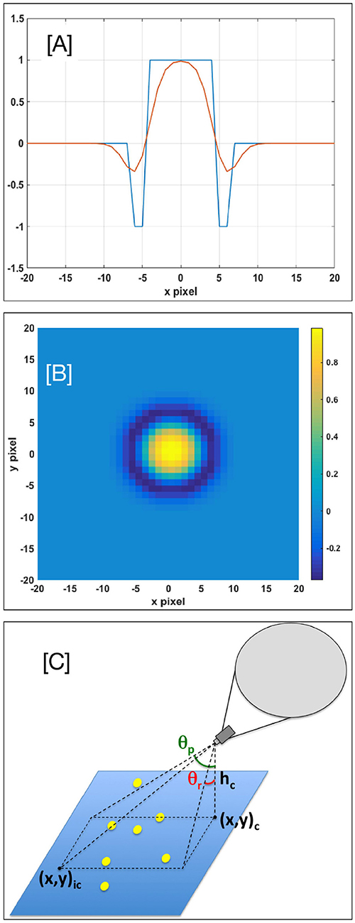
Figure 3. (A) Cross-section of the kernel along the x-axis showing the step function in blue and the Gaussian smoothed shape in red. (B) Kernel of the shape filter used to identify individual bamboo plates. (C) Schematic diagram of the relevant quantities used to rectify STARSS imagery. Here, θp, θr, hc, (x, y)c, and (x, y)ic correspond to pitch, roll, heading, altitude, camera position, and image center, respectively. See Equation 6 in section 2.4.2.
The next step is color-filtering. Relative to the open-ocean seawater, whose hues are dominated by blue, and the sun glitter, whose colors are close to pure white, the plates are characterized by yellow, red, and magenta colors. This property is exploited in the conversion of the three RGB color components into a single intensity value, using the function
where r, g, and b are color components of each pixel (Figures 4A,B).
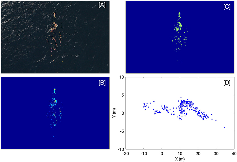
Figure 4. (A) A raw RGB image excerpt showing the patch of bamboo plates. (B) A grayscale image produced after the color filtering step (see Equation 1 in section 2.4.1) clearly separates the patch of plates from the background and removes sun glitter. (C) The binary image (plates = 1 and background = 0) that results after the thresholding step. (D) The rectified patch of plates, with the major axis oriented along the x-axis due to lack of heading data.
For the patch deployments, it is sometimes helpful at this stage to perform a noise filter to eliminate sun glitter. This can be done, e.g., with a bandwidth or a Wiener filter; here the MATLAB implementation wiener2 is used with a 200 × 200 window. Knowing the approximate number of plates released and the approximate number of pixels per plate, one can estimate the total number of plate pixels. A binary image is created by setting the brightest pixels to 1 and others to 0 (Figure 4C). The best threshold value depends on the particular experiment, but tends to be around 0.05 or 0.025%.
The last step is to identify the approximate plate centers. This is done following the method of Crocker and Grier (1996), in an implementation based on that by Blair and Dufresne (http://site.physics.georgetown.edu/matlab/). After all local maxima are found within a local neighborhood of approximate plate size, the collection is thinned with a minimum imposed separation of one plate radius. The center position is then refined as the intensity-weighted centroids of the pixels within the local neighborhoods of the local maxima. For patches, this procedure yields a nearly uniform distribution of identified plates within each patch. In some applications, it is preferred to deal with these bright areas in the image as a single patch instead of as a collection of “plates" whose number is highly dependent on the chosen exclusion radius. In these cases, the MATLAB functions bwconncomp and regionprops can extract the properties of the individual contiguous areas, including their centroids and their areas, which are estimates of the number of plates within each patch.
2.4.2. Absolute Rectification
Absolute rectification, or direct georectification, uses the horizontal position, altitude, orientation (pitch, roll, and heading), and camera parameters (sensor size and resolution and lens focal length) to assign a geographic location to each pixel in the image (Mostafa and Schwarz, 2001). Here we summarize the basic principals of direct/absolute georectification of low-altitude aerial imagery as they relate to an unstabilized camera suspended from an aerostat.
Since the camera was mounted on an aerostat, which was tethered to a heaving, surging, and swaying ship, the camera was always in motion (translating, and rotating about all three axes). The position, altitude, and orientation data recorded by the INS were collected with the intention of using them to directly georectify the images. However, the magnetometer on the INS malfunctioned and incorrect heading data were recorded. Other variables output by the EKF used by the INS, i.e., horizontal position, altitude, pitch, and roll, depend on the accuracy of all the input data and, therefore, may have been affected as well. Figure 3C shows a diagram of the aerostat and camera relative to its field of view and the variables required to directly georectify aerial imagery.
Ideally, one can calculate the absolute position of each plate in an image given complete information about the camera motion. First, in pixels relative to the center of the image (xi, yi) plate coordinates are converted to look angles at the camera (αx, αy):
lx, ly are sensor dimensions (36 × 24 mm for the full-frame sensor in the Canon EOS 5DSR Mk III), Nx, Ny are image dimensions in pixels (8, 688 × 5, 792), and f is the focal length of the lens (17–21 mm).
These angles, after adjustment for camera pitch (θp), roll (θr), and heading (θh) are then converted to position relative to the camera (), which is in turn converted to absolute position ().
where hc is camera altitude, xc is camera position, and R(θh) is the 2D rotation matrix.
2.4.3. Relative Rectification
Camera motion information may be unavailable, incomplete, or inaccurate. When this is the case, it is still possible to perform a “relative" rectification, finding positions of plates relative to the centroid of the collection of plates (Figure 4D). Relative rectification builds on the assumption that the plates move only small distances between consecutive frames and that large apparent motion of the entire field of plates is due to camera motion. Since images were collected every 15 s, this assumption is reasonable. Note, however, that relative rectification removes large-scale coherent motion of the group of plates. Therefore, positions obtained through relative rectification can be used to analyze relative dispersion but not absolute dispersion. The process translates and rotates the field of plates such that the total movement of all plates from one frame to the next is minimized. Even when absolute rectification is possible, this relative rectification may be used to improve the performance of the plate linking algorithm (see section 2.4.4).
Given plate positions at time t, the following minimization determines translation and rotation θ to be applied to plate positions in the next image from time t + Δt:
where N(t) is the number of plates in the image at time t.
For the inner minimization of Equation (7), we used the MATLAB nearest neighbor search function knnsearch. For the outer minimization of (7), we used the MATLAB function fminsearch, which searches for local minima using the simplex search method of Lagarias et al. (1998). Specifying a reasonable start value for the search is important. The initial value of is taken to be the translation that maps the center of mass of the field of plates to the origin. The center of mass of is also at the origin and its major axis aligned with the x-axis. If necessary, the initial value for θ can be chosen as the smaller of the two angles such that the primary eigenvector of the position covariance matrix C(t + Δt) aligns with the x-axis. The covariance matrix is
where averaging 〈·〉 is over all the plates at time t. However, for plate dispersion experiments with a preferred direction of motion, like the front described in section 3, this rotation is not necessary.
Despite our best efforts, some sun glitter may be falsely detected as “plates.” Unlike real plates, which persist from frame to frame and move relatively short distances, sun glitters are ephemeral and change depending on waves, clouds, and camera orientation. Therefore, distances between sun glitters from one frame to the next tend to be larger than distances traveled by plates. Because the experiments were set up to minimize plates in areas of strong sun glitter, glitters also tend to be farther away from plates. Thus, the false positions can, to some extent, be removed with a distance threshold to the closest plate. In order to avoid including sun glitters in the minimization itself, the summation in Equation (7) can be re-written to exclude the M largest “plate" distances, where M is chosen to be some small fraction of the total number of plates N. We used a distance threshold of 3.4 m and fraction M/N = 0.1.
2.4.4. Linking and Particle Tracking
Once the rectified plate positions in each frame have been determined, plate trajectories can be constructed by linking individual plates between frames. The linking procedure creates one-to-one associations (links) between plates from frame to frame such that the total distance between plates in consecutive images is minimized (Malik et al., 1993; Chenouard et al., 2014). While both the relative rectification and linking procedures minimize total distance between plates, they differ in that rectification transforms the plate fields (as described in section 2.4.3) while linking does not, and linking produces one-to-one associations between plates while relative rectification does not. We used a MATLAB linking algorithm called “Simple Tracker" by Jean-Yves Tinevez (https://www.mathworks.com/matlabcentral/fileexchange/34040-simple-tracker).
Linking performance degrades when the non-dimensional spacing becomes small or as position errors due to uncorrected camera motion become large relative to displacement (uΔt; Malik et al., 1993). While the Simple Tracker has some ability to deal with data gaps when a plate is not detected for a frame but reappears in the next frame, the trajectories derived with this method for the sample grid deployment nonetheless tended to be relatively short, with an average time span of 52 min, compared to the total length of the experiment, which was approximately 170 min. On average, plate spacing was Δx ≈ 3.4 m, the time between images was Δt = 15 s, and the average velocity was u ≈ 0.022 ms−1, which results in average P ≈ 10. However, P-values can be significantly smaller, because maximum velocities may reach u ≈ 0.22 ms−1, and plate spacing Δx decreases to < 0.5 m as the plates cluster together. Plate velocities were calculated by forward differencing of plate positions along trajectories. In order to detect and eliminate erroneous velocities due to incorrect links, each velocity which differs by more than 2 standard deviations from the average velocity in its neighborhood is eliminated from the statistics. We used the default 6.8 m for neighborhood radius.
2.4.5. Dispersion Metrics
The evolution of the patch was quantified by computing the dispersion, the relative dispersion of pairs of plates, and the relative diffusivity. Dispersion ellipses, σ2, were fit to the patch of plates in each image for comparison with the results of Okubo (1971). Ellipse-fitting is not affected by the time interval between images or the number of plates detected and simply computes the variance along the major and minor axes of the patch of plates (Okubo, 1971). If σa and σb denote the variances of the distribution of plates along the major and minor axes, respectively, then
Indication of the presence of coherent structures comes from the anisotropy of the flow field and is revealed by anisotropy in the dispersion rates. σa and σb are, therefore, computed separately, and the ratio is used to identify incidences of anisotropic dispersion.
While Equation (9) provides a relatively simple method to quantify the dispersion of a patch of plates, it does not provide any information about the motions of individual plates inside the patch. Trajectories of individual plates (see section 2.4.4), on the other hand, can be used to compute the relative dispersion by examining pairs of initially proximal plates. Relative dispersion is computed as
where r is the position vector and plate pairs are indicated by subscripts. The relative dispersion provides a measure of the separation of initially proximal plates at a given time (LaCasce, 2008) and is commonly used when analyzing large numbers of trajectories of virtual particles computed from numerical ocean model (e.g., Haza et al., 2014) or HF radar velocity fields (e.g., Carlson et al., 2010), and in limited cases when sufficient numbers of drifter observations exist (e.g., LaCasce and Ohlmann, 2003; Poje et al., 2014).
Following Okubo (1971) we compute diffusivity (K) from dispersion
Spatial bin averaging of K was performed using 5 m bins for plates and 20 m bins for surface drifters. Bootstrap estimates of the mean (Efron and Tibshirani, 1986) and their 95% confidence intervals were computed.
3. Results
3.1. Experiment Setting
The STARSS dispersion experiment discussed here took place on 30 January 2016 approximately 130 km southeast of the Mississippi River Delta in a depth of approximately 140 m near the region described by D'Asaro et al. (2018). The front to be targeted, extending from northeast to southwest, was detected in the aerial SST mosaic (Figure 5), and its precise position could be followed in real-time in the X-band radar backscatter data (Figure 6). Post-processed X-band radar surface currents (see section 2.3.4) showed that velocities were stronger (0.4 ms−1) on the western side of the front and directed toward the southwest (Figure 6). Velocities on the eastern side of the front were somewhat weaker (0.2–0.3 ms−1) and were directed toward the west (Figure 6). The thermosalinograph on the R/V Walton Smith showed that near-surface water was colder and fresher on the west and warmer and saltier on the east side of the front (Figure 7). On larger spatial scales, surface drifter trajectories indicate that the front extended at least 140 km (Figure 8). Some of these drifters were observed in the front by aerostat operators on the bridge of the M/V Masco VIII during the dispersion experiment, along with patches of sargassum and freshwater vegetation.
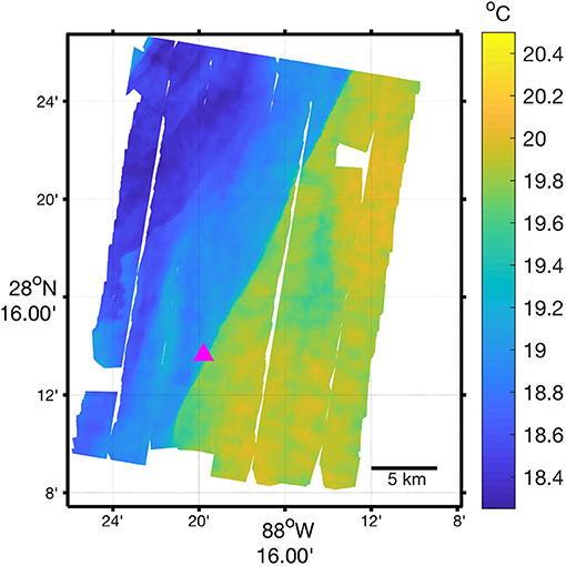
Figure 5. An aerial SST mosaic (section 2.3.5) of the area targeted during the STARSS experiment (magenta triangle) shows a sharp front that extends from the northeast to the southwest, with colder water on the west and warmer water on the east side of the front.
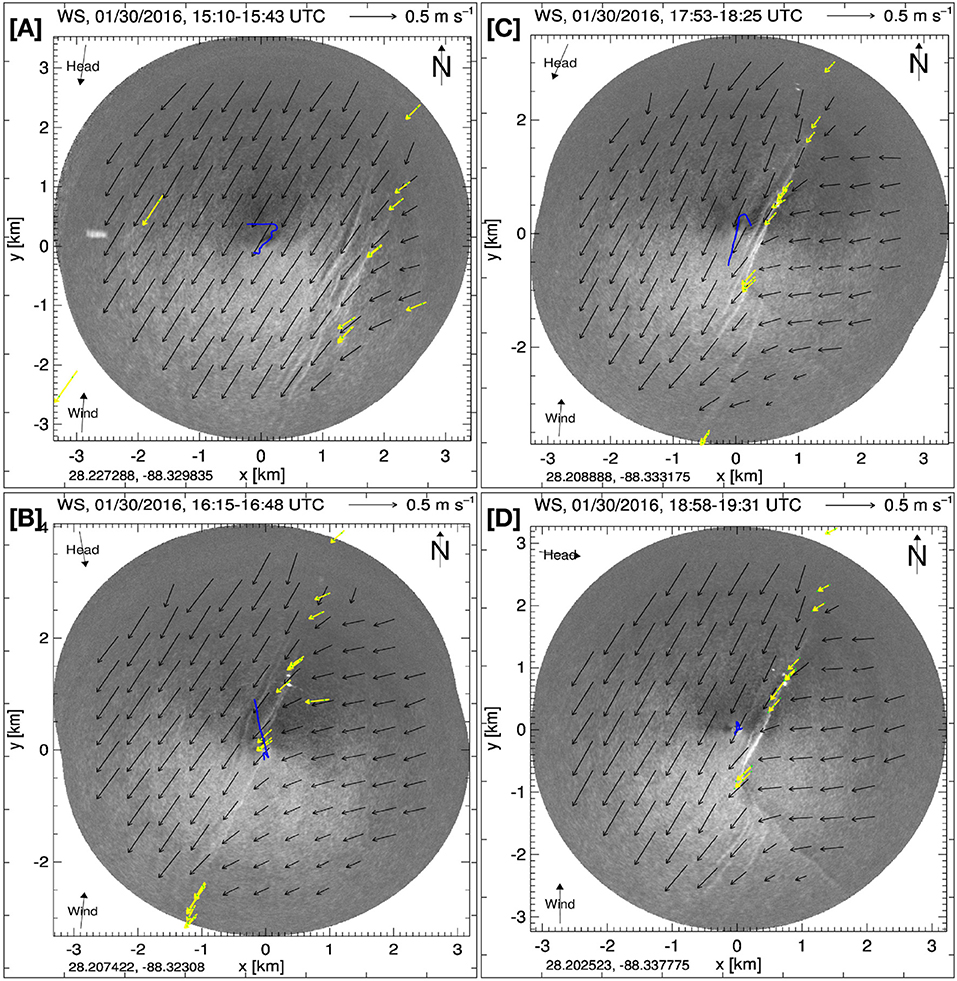
Figure 6. A–D show the orientation of a density front that was targeted during the STARSS dispersion experiment on 30 January 2016. The front is visible in normalized marine backscatter intensity (greyscale; see section 2.3.4). Surface currents (black arrows), surface drifter trajectories (yellow arrows) and the ship track (blue) are also shown during the averaging period for each frame. The black arrows in the image corners indicate image heading, mean ship heading, and wind direction (counterclockwise from top right). (A) shows the front at approximately 30 min prior to the beginning of the STARSS experiment. The radar data shown in panels B–D correspond to times of 7 min, 105 min, and 170 min in Figures 9–12.
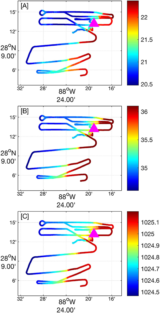
Figure 7. Sea surface temperature (A), salinity (B), and density (C) recorded by the thermosalinograph on the R/V Walton Smith. The starting location of the STARSS dispersion experiment is indicated by the pink triangle.
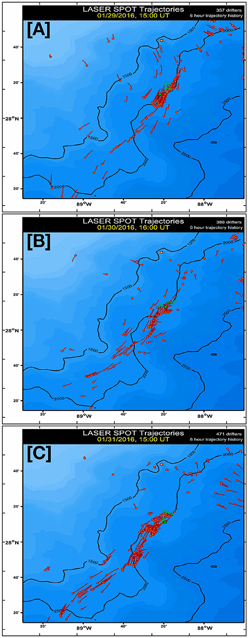
Figure 8. Trajectories of LASER surface drifters deployed in the region on (A) 29 January, (B) 30 January, and (C) 31 January reveal the scale of the front sampled by STARSS. The tails correspond to the previous 6 hr positions and the green line corresponds to the R/V Walton Smith's position.
The large-scale drift of the patch of plates is inferred from drifter trajectories, before, during, and after the STARSS experiment, and the trajectories recorded by GPS receivers on three wave buoys (see section 2.3.3) that were deployed in the patch of plates. The drifter and wave buoy trajectories show a general drift to the southwest (Figure 8). The average speed of the wave buoys was 0.15–0.18 ms−1, with maximums of 0.25 and 0.28 ms−1 observed in two buoys at the end of the experiment (Figure 9A). The wave buoys remained in the patch throughout the entire experiment despite their spherical shape and large (when compared to plates) above-water surface area that could have been subject to windage.
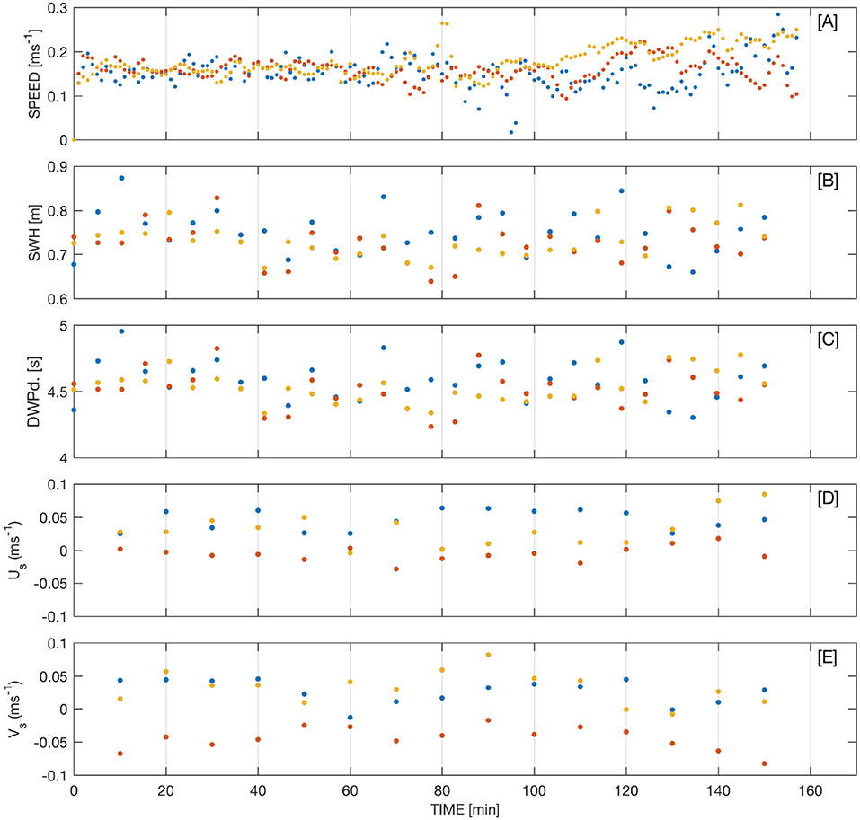
Figure 9. (A) Drift speed of each wave buoy. (B) Significant wave height (SWH) and (C) dominant wave period (DWPd). The zonal and meridional components of the surface Stokes drift are plotted in (D,E), respectively.
Significant wave heights during the experiment were generally small (< 1 m) and the dominant wave period was approximately 4–5 s (Figures 9B,C). The surface Stokes drift ranged from 0.05 to 0.1 ms−1 during the experiment (Figures 9D,E). The meridional surface Stokes drift velocities suggest that buoy 2 (red dots in Figure 9E) and buoys 1 and 3 (blue and yellow dots in Figure 9E) were on opposite sides of the front due to the consistently opposite signs of their respective velocities. The Langmuir number (see Equation 4 in Thorpe, 2004) was approximately 0.01 throughout the experiment, which is typical of the open ocean and indicates that the development of Langmuir circulation (LC) was possible. The turbulent Langmuir number, Lat,
was approximately 0.39 throughout the experiment (McWilliams et al., 1997). In Equation 12, U* is the friction velocity (, where τ and ρ are the wind stress and density of seawater, respectively) and us is the surface Stokes drift. The windrows commonly associated with LC were not observed in STARSS imagery during this experiment. LC was observed during a STARSS experiment that was conducted 6 February 2016, and it will be discussed in detail in a forthcoming publication.
Winds were primarily from the west-northwest to the east-northeast (Figures 10A,B). The two strongest wind events, where wind speeds exceeded 9 ms−1, had strong southerly components and were recorded during the first 30 min of the experiment (Figures 10C,D). These events, however, were short-lived, lasting < 5 min. A 6 min westerly wind event was recorded approximately 150 min into the experiment (Figure 10C). Throughout much of the experiment, the meridional component of the wind velocity remained northerly while the zonal component was variable and changed sign quite often (Figure 10C).
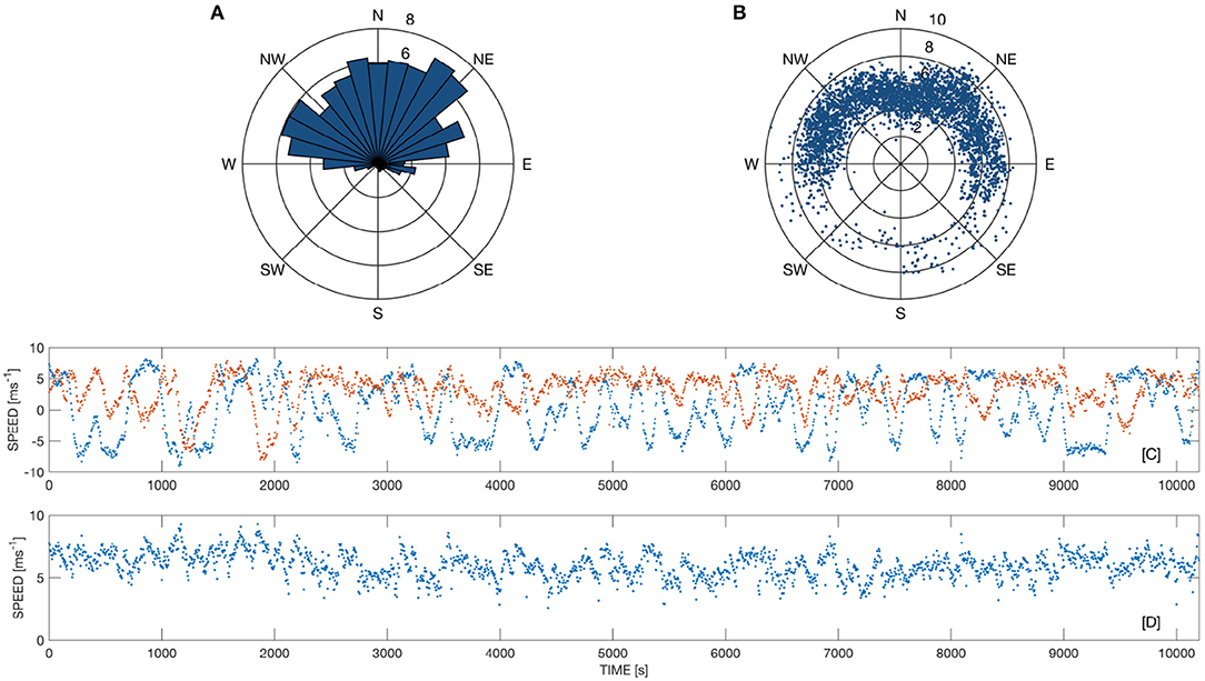
Figure 10. (A) Direction frequency, or wind rose, of winds recorded on the M/V Masco VIII during the STARSS experiment. (B) Directional distribution of wind speeds. Time series of: (C) the zonal (blue) and meridional (red) components of the wind vector and (D) wind speed.
3.2. Plate Dispersion
A patch of plates was released near the front by a small work boat and was imaged by STARSS for nearly 4 hr, though the analysis presented here was limited to a 170 min segment. The analysis began after the last plates were deployed and continued until the elongation of the patch exceeded the FOV of the imagery. A 17 mm focal length was used during this experiment, which corresponds to nadir-looking image dimensions of 318 × 212 m. The INS recorded incorrect heading data, the cause of which is discussed in section 4, and, as a result, the STARSS images were rectified using a combination of absolute and relative rectification. First, absolute rectification (section 2.4.2) was performed using the horizontal position, altitude, pitch, and roll. Given the lack of accurate heading data and precise synchronization between the camera and the INS, two relative rectification (section 2.4.3) passes were used. Between 250 and 290 individual plates were detected in each image, which enabled plate positions to be linked (section 2.4.4). However, changes in illumination and camera settings resulted in two gaps in the rectified image sequence where insufficient contrast between the ocean surface and the plates led to poor performance of the detection algorithm (see section 2.4.1). While these detection gaps did not pose a problem for cloud dispersion estimates, they resulted in three sets of trajectories for linked plates.
Figure 11 shows snapshots of the rectified plate positions and Supplementary Video 1 shows the evolution of the patch of plates over the 170 min experiment. Shortly after deployment the patch began to contract and it reached its minimum area at 5 min (Figure 11B). At approximately 16 min it began to stretch into a streak, reaching its maximum length at 36 min (Figure 11C). The patch then contracted and varied in size until the 112 min mark (Figure 11D), after which time it stretched rapidly, forming a long, narrow streak (Figure 11E). From that point until the end of the analysis period (170 min) the streak deformed into a curved shape (Figure 11F). At the end of the experiment the front appeared to break down and the plates spread rapidly both along and across the front and many plates either left the FOV or were influenced by the M/V Masco VIII. Westerly winds (Figure 10C) may have contributed to the apparent breakdown of the front, which was observed from 141 to 170 min (Figure 11F and Supplementary Video 1).
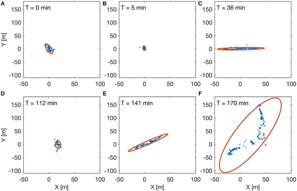
Figure 11. Snapshots of rectified plate positions and ellipses at (A) 0 min, (B) 5 min, (C) 36 min, (D), 112 min, (E) 141 min, and (F) 170 min. Supplementary Video S1 shows all rectified plate positions.
Cloud dispersion of the entire patch of plates was computed using Equation 9 and the relative dispersion (RD) of pairs of plates was computed using Equation 10. The temporal evolution of the dispersion of the patch of plates and the root-mean-square (RMS) average of the RD is shown in Figure 12A. The contraction observed after deployment (Figure 11B) is evident in a gradual decrease in cloud dispersion and RMS RD from 0 to 5 min (Figure 12A). A power law fit to the cloud dispersion over the interval 5–16 min suggests quasi-diffusive dispersion with σ2 ~ t0.63 (determined by a power law fit to the subset of data using Matlab's curve fitting tool; R2 = 0.91). The RMS RD during this same interval remained relatively stable and did not exhibit any clear power law dependence. The elongation of the patch into a streak from 16 to 36 min (Figure 11C) is reflected in super-Richardson regimes for both cloud dispersion (σ2 ~ t6.8; R2 = 0.97) and RMS RD (; R2 = 0.96). The contraction and variability from 36 to 112 min is also clearly evident in both the cloud dispersion and RMS RD. The rapid spread observed from 112 to 170 min is evident in power law fits to both dispersion metrics, with exponents of 14.9 (R2 = 0.93) and 8.8 (R2 = 0.97) for cloud dispersion and RMS RD, respectively.
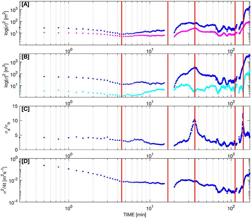
Figure 12. (A) Cloud dispersion, of the patch of plates (blue dots) and average relative dispersion of pairs of plates (pink dots) plotted as a function of time on a logarithmic scale. (B) The major and minor axes of the dispersion ellipses are denoted by dark blue and cyan colors, respectively. (C) The dispersion ratio σa/σb. (D) The diffusivity () computed from Equation 11. Vertical red lines correspond to snapshots in Figure 11 and times mentioned in the text.
The major and minor axes of the dispersion ellipses and their ratio (σa/σb), or the dispersion ratio, are plotted in Figures 12B,C. The ratio of major and minor dispersion ellipses show anisotropic dispersion due to the front throughout the experiment (Figure 12C) with two peaks at 36 and 141 min that corresponded to the super-Richard dispersion regime that was noted above. The dispersion ratio decreased rapidly from 141 to 170 min, during the apparent breakdown of the front, as plates spread in both the along and cross-front directions (see Supplementary Video 1).
The relative diffusivity, K, also exhibited large temporal variability (Figure 12D). The initial K of 0.49 m2s−1 declined to 7.0 × 10⁻³ m2s−1 as the patch of plates contracted during the first 5 min (Supplementary Video 1). K increased to 1.1 × 10⁻² m2s−1 during the first elongation into a streak (16–36 min). Diffusivity then decreased, reaching 9.5 × 10⁻⁴ m2s−1 at 112 min and then rapidly increased to 4.0 × 10⁻² m2s−1 at 170 min. The scale-dependent diffusivity computed from the dispersion ellipses (Equation 11) shows that the STARSS experiment resolved spatial scales from 3 m to 42 m (Figure 13A). However, the scatter at the smaller scales (3–10 m) and during the first 42 min of the experiment suggests no clear dependence of K on separation scale (Figure 13A). The bin averaged diffusivity (see section 2.4.5), on the other hand scales as K = 2.1 × 10⁻⁴L1.44 (R2 = 0.98; Figure 13A).
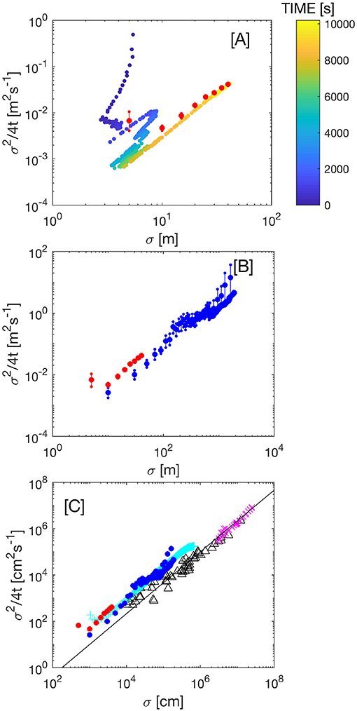
Figure 13. (A) STARRS scale-dependent diffusivities, color-coded according to time since deployment, and bin-averaged diffusivities (red dots). (B) Bin averaged STARSS (red) and surface drifter (blue) diffusivities. The large dots represent bootstrap estimates of the mean and the vertical lines represent 95% confidence intervals. (C) Previous results Okubo (1971), Poje et al. (2014), and Mensa et al. (2015) are represented by black triangles, pink ‘x’s, and light blue ‘ + 's. Richardson scaling (K ~ σ4/3) is shown as a solid black line.
3.3. Surface Drifter Dispersion
LASER surface drifter trajectories were used to compute relative dispersion and relative diffusivity to extend the STARSS results to the submesoscale. A subset of drogued surface drifter trajectories was extracted from the quality-controlled LASER drifter dataset (D'Asaro et al., 2017; Haza et al., 2018). Three-day trajectories of those drogued surface drifters that were within 10 km of the STARSS experiment location at its beginning were extracted from the quality-controlled and interpolated LASER drifter data set (D'Asaro et al., 2017; Haza et al., 2018). Of these 53 trajectories, 21 drifter pairs with an initial separation < 150 m were identified. The RD, relative diffusivity, and bin-averaged relative diffusivity of each drifter pair were computed (see section 2.4.5). The surface drifters resolved dispersion over scales of 10–1,630 m during the 3 day period considered (Figure 13B). A power law fit to the data suggests the drifter diffusivities scaled as K = 2.1 × 10⁻⁵L1.65 (R2 = 0.49). When compared with the STARSS plate results the bin averaged drifter diffusivities show consistent scaling over the entire range of spatial scales resolved (Figure 13B). Figure 13C shows that the scale dependence agrees well with Richardson's 4/3 law, as well as with the dye-based results of Okubo (1971), GLAD surface drifter results from Poje et al. (2014), and LES results of Mensa et al. (2015).
4. Discussion
4.1. STARSS Dispersion Results
The temporal evolution of the cloud dispersion and RD do not exhibit a local Richardson dispersion regime (σ2 ~ t3) and, instead, show periods of quasi-diffusive and super-Richardson dispersion (Figure 12A). The bin-averaged diffusivities, on the other hand, exhibit a clear dependence on scale that agrees well with Richardson's 4/3 law and previous observational and numerical results (Figure 13C). Richardson scaling, however, emerged from spatial bin-averaging diffusivity estimates from the entire experiment while the periods of super-Richardson dispersion were short-lived, O(10 min), and corresponded to periods of strong anisotropic dispersion (Figures 12B,C). Individual diffusivity estimates exhibited significant scatter, especially in the 3–10 m scales (Figure 13A). Scatter is to be expected in observational estimates of diffusivity and can be due to the complex flow field, surface waves, anisotropic turbulence and the fact that the plates were constrained to the sea surface and did not resolve three dimensional turbulent motions (Salazar and Collins, 2009).
The STARSS observations presented here extend observational estimates of scale-dependent diffusivity down to 3 m (Figure 13). The bin-averaged diffusivities exhibit a clear scale dependence, which agrees well with a coastal study by Matsuzaki and Fujita (2017) who tracked drifting buoys and rubber mats. The range of diffusivities (10−4 m2s−1 to 0.4 m2s−1) agree with other observations at similar spatiotemporal scales (Li, 2000; Carlson et al., 2010; Matsuzaki and Fujita, 2017). The STARSS diffusivity of 0.4 m2s−1 observed at 40 m and Okubo's diffusivity of 0.5 m2s−1 observed at 100 m (Figure 13C) show reasonable agreement, which suggests that diffusivities of this magnitude can be expected at these scales. This agreement is striking when considering that Okubo (1971) analyzed the three-dimensional spread of dye releases, which are known to behave differently than near surface 2D motion (Mensa et al., 2015).
4.2. STARSS Performance
STARSS met its design requirements (see section 2.2) and satisfied the overall objective of quantifying small-scale, surface ocean dispersion in an open ocean environment, as evidenced by the results of a dispersion experiment that was conducted along a density front in the northern Gulf of Mexico. The plate detection algorithms were able to distinguish between bamboo plates and ephemeral features like sun glitter and white caps (see section 2.4.1). The use of painted plates had no discernible effect on detection success. Aerial images of plates were rectified using a combination of absolute rectification (see section 2.4.2) and relative rectification (see section 2.4.3) methods. Dispersion ellipses (Equation 9) quantified the spread of the entire patch of plates, and the relative dispersion (Equation 10) quantified the separation between individual pairs of plates.
The main drawbacks of STARSS were INS performance and the size of the aerostat. The Inertial Labs INS was selected as a compromise between cost and accuracy (MEMS-based sensors are significantly cheaper, though much less accurate, than fiberoptic gyro IMUs). Unfortunately, the INS did not function as specified due to initialization errors. Inertial Labs replaced the INS with an improved version that is designed for rapid initialization on moving platforms. The INS also lacked an event trigger, hindering precise synchronization of the imagery with the INS data. Approximate absolute rectification was performed, followed by a relative rectification (see section 2.4.3), which increased the data analysis requirements and processing time. The relatively large size and weight of the INS made it difficult to mount on the camera and the combined weight of the camera, lens, and INS prohibited the use of a gimbal for image stabilization.
The large envelope of the aerostat provided 30 kg of lift, which was sufficient to lift the 10 kg onboard instrumentation (Figure 1A). The lift safety factor allowed the safe recovery of the aerostat and instruments when the emergency deflation device was mistakenly triggered. However, the lift requirements of the aerostat required a relatively large number of helium cylinders to be stored onboard the M/V Masco VIII and the combined lift and drag of the aerostat required a custom electric winch for retrieval. The winch, however, lacked the torque required to reel in the aerostat when wind speeds exceeded 10 ms−1. This problem could be solved by upgrading the winch but decreasing the lift requirement would enable the use of a smaller aerostat, which would have the added benefits of reducing the amount of helium required to inflate the aerostat, which could, in turn, permit the use of a smaller winch and allow for deployments from smaller vessels.
The heaviest components were the full-frame DSLR, sealed lead acid batteries, and the aluminum frame. The 50.6 megapixel Canon 5DSR Mk III DSLR was selected because of its resolution and image quality. Analysis of half-resolution images produced identical results when compared to full-resolution images, which suggests that a smaller, lighter, and cheaper mirrorless camera could be used in future studies. Use of lithium polymer (LiPo) batteries and a carbon fiber frame would also result in significant reductions in weight. A mirrorless camera and a small INS with an event trigger would also permit the use of a gimbal in future studies, though even a stabilized camera will be subject to heave, sway, and surge due to wind gusts and ship motion transmitted through the tether.
Since STARSS development began UAS flight capabilities and cameras have improved dramatically. UAS flights would allow the tender vessel to stay well clear of the patch of bamboo plates. Most commercially available UAS, however, were developed for cinematography and agricultural monitoring and, therefore, may require some modifications before they are suitable for use at sea. Unlike tethered aerostat flights, which do not require licenses or certifications, research-related UAS operations are considered non-recreational by the FAA and require a commercial remote pilot certificate. Thus, we argue that aerostats offer a safe and stable aerial platform that are relatively simple to operate. For example, complete power loss on STARSS had no effect on the flight characteristics of the aerostat while power loss on a rotary-wing UAS would result in a crash and, therefore, significantly increases the risk of a complete loss of the system. Based on our experience, we recommend that a future implementation of a STARSS-like system address its short-comings as suggested above. In particular, integration of UAS imaging and communications systems into a STARSS-like system could provide the convenience of “plug-and-play” hardware and software with the stability of an aerostat.
5. Summary and Conclusions
This paper presents the development and deployment of the ship-tethered aerostat remote sensing system, data analysis techniques, and results of a dispersion experiment that was conducted at an offshore density front in the northern Gulf of Mexico on 30 January 2016. The front was detected in aerial SST imagery (section 2.3.5) and tracked by a scientific X-band radar (section 2.3.4). A patch of plates was deployed on the front, and STARSS documented the evolution of the patch for 170 min (section 3). The contraction and dilation of the patch of plates was quantified by computing the dispersion of the entire patch and by computing the relative dispersion from plate trajectories (Figure 12). The small-scale STARSS observations were connected to the submesoscale using surface drifter trajectories and, when viewed together, the scale-dependent dispersion suggest that Richardson's 4/3 scaling persists over the range of spatiotemporal scales sampled: 10–1,600 m and minutes to 3 days (Figure 13C). In short, the presence and persistence of the front resulted in anisotropic dispersion, that was observed in both surface drifters and plates down to spatial scales of O(10 m), which highlights the importance of resolving dispersion from the submesoscale down to oceanic boundary layer turbulence scales. The apparent breakdown of the front at the end of the STARSS experiment (Figure 11F and Supplementary Video 1) also reveals focus areas for future research. The reason for the rapid dispersal of plates away from the front is not known. Given a Langmuir number of 0.01, this behavior could have been due to the onset of Langmuir circulation (LC) as wind speed increased and wind direction shifted to cross-front (Figure 10 and Supplementary Video 1). However, the windrows commonly associated with LC were not observed in STARSS imagery during this experiment. LC was observed during a STARSS experiment that was conducted 6 February 2016, and it will be discussed in detail in a forthcoming publication.
To the best of our knowledge, this is the first observational attempt to simultaneously resolve surface ocean Lagrangian dispersion at oceanic boundary layer scales and submesoscales. STARSS-like observations can be easily replicated and integrated into existing and planned field campaigns. However, we stress that we do not expect STARSS to be duplicated exactly and any combination of sensors and aerial platforms that can satisfy the requirements summarized in Table 1 can be used. Given the popularity of UAS for low-altitude remote sensing applications we can expect improved performance in terms of size, weight, and power in positioning systems, camera systems, and aerial platforms, which, at the very least, would permit a smaller aerostat to be used. As UAS become more reliable, capable, and affordable they can also be a viable alternative to an aerostat for studies of surface ocean dispersion. While some flexibility certainly exists in the choice of aerial platform, imaging system, and positioning system, the data analysis workflow presented in section 2.4 can be applied to any imagery of drifting objects on the sea surface, which will help fill a critical knowledge gap about how the ocean transports material at the sea surface and at small spatiotemporal scales and will enable observations of dispersion to be obtained throughout the world's oceans. In addition to improving our response tactics to oil spills, these results can aid in understanding oceanic boundary layer turbulence in general and complement numerical and laboratory studies of turbulent dispersion.
Author Contributions
DC, TÖ, GN, CG, HC, MB, MC, ER, and LB aided in the development, construction, and testing of STARSS. DC, TÖ, GN, CG, JM, SM, HH, MB, and MR participated in the LASER experiment. DC, HC, BF-K, JM, EF, HH, and AK developed image analysis algorithms. BL and JH provided X-band radar data. SM and BH provided meteorological and wave buoy data. JM provided georectified aerial SST data. MC and SC provided coupled-model forecasts. All authors contributed to overall experimental design, interpretation of results, and editing of the manuscript.
Funding
This research was made possible by a grant from The Gulf of Mexico Research Initiative. STARSS data (doi: 10.7266/N7M61H9P), surface drifter data (doi: 10.7266/N7W0940J), meteorological data (doi: 10.7266/N7S75DRP), aerial SST data (doi: 10.7266/N7280608), and X-band radar data (doi: 10.7266/N7N01550) are publicly available through the Gulf of Mexico Research Initiative Information & Data Cooperative (GRIIDC) at https://data.gulfresearchinitiative.org. Early aerostat test flights were made possible through ship time provided by The International Seakeepers Society.
Conflict of Interest Statement
The authors declare that the research was conducted in the absence of any commercial or financial relationships that could be construed as a potential conflict of interest.
The reviewer AJ declared a shared affiliation, with no collaboration, with one of the authors, MC to the handling editor at time of review.
Acknowledgments
We thank J. Beckman and J. Pilgrim and of the Federal Aviation Administration and the Lockheed Flight Services staff for their assistance in coordinating aerostat flight operations in the Gulf of Mexico. We also thank B. Gullett of the Environmental Protection Agency for his advice in planning ship-based aerostat operations. We also thank the students and staff from the Rosenstiel School for Marine and Atmospheric Sciences who assisted either with STARSS development or with dispersion experiments during the LASER cruise. Finally, we thank students in Miami-area schools for painting bamboo plates.
Supplementary Material
The Supplementary Material for this article can be found online at: https://www.frontiersin.org/articles/10.3389/fmars.2018.00479/full#supplementary-material
References
Anctil, F., Donelan, M., Drennan, W., and Graber, H. (1994). Eddy-correlation measurements of air-sea fluxes from a discus buoy. J. Atmos. Oceanic Technol. 11, 1144–1150. doi: 10.1175/1520-0426(1994)011<1144:ECMOAS>2.0.CO;2
Aurell, J., and Gullett, B. (2010). Aerostat sampling of PCDD/PCDF emissions from the Gulf oil spill in situ burns. Environ. Sci. Technol. 44, 9431–9437. doi: 10.1021/es103554y
Bachman, S., Fox-Kemper, B., Taylor, J., and Thomas, L. (2017). Parameterization of frontal symmetric instabilities. I: Theory for resolved fronts. Ocean Modell. 109, 72–95. doi: 10.1016/j.ocemod.2016.12.003
Berta, M., Magaldi, M., Özgökmen, T., Poje, A., Haza, A., and Olascoaga, J. (2015). Improved surface velocity and trajectory estimates in the Gulf of Mexico from blended satellite altimetry and drifter data. J. Atmos. Oceanic Technol. 32, 1880–1901. doi: 10.1175/JTECH-D-14-00226.1
Bezerra, M., Diez, M., Medeiros, C., Rodriguez, A., Bahia, E., Sanchez-Arcilla, A., et al. (1997). Study on the influence of waves on coastal diffusion using image analysis. Appl. Sci. Res. 59, 191–204. doi: 10.1023/A:1001131304881
Braun, N., Ziemer, F., Bezuglov, A., Cysewski, M., and Schymura, G. (2008). Sea-surface current features observed by Doppler radar. IEEE Trans. Geosci. Remote Sens. 46, 1125–1133. doi: 10.1109/TGRS.2007.910221
Brouwer, R., de Schipper, M., Rynne, P., Graham, F., Reniers, A., and MacMahan, J. (2015). Surfzone monitoring using rotary wing unmanned aerial vehicles. J. Atmos. Oceanic Technol. 32, 855–863. doi: 10.1175/JTECH-D-14-00122.1
Callies, J., and Ferrari, R. (2018). Baroclinic instability in the presence of convection. J. Phys. Oceanogr. 48, 45–60. doi: 10.1175/JPO-D-17-0028.1
Carlson, D., Fredj, E., Gildor, H., and Rom-Kedar, V. (2010). Deducing an upper bound to the horizontal eddy diffusivity using a stochastic Lagrangian model. Environ. Fluid Mech. 10, 499–520. doi: 10.1007/s10652-010-9181-0
Carrier, M., Ngodock, H., Smith, S., Muscarella, P., Jacobs, G., Özgökmen, T., et al. (2014). Impact of assimilating ocean velocity observations inferred from Lagrangian drifter data using the NCOM-4DVAR. Mon. Weather Rev. 142, 1509–1524. doi: 10.1175/MWR-D-13-00236.1
Chenouard, N., Smal, I., de Chaumont, F., Maška, M., Sbalzarini, I. F., Gong, Y., et al. (2014). Objective comparison of particle tracking methods. Nat. Methods 11, 281–289. doi: 10.1038/nmeth.2808
Clarke, A., and Van Gorder, S. (2018). The relationship of near-surface flow, Stokes drift and the wind stress. J. Geophys. Res. Oceans 123, 4680–4692. doi: 10.1029/2018JC014102
Coelho, E., Hogan, P., Jacobs, G., Thoppil, P., Huntley, H., Haus, B., et al. (2015). Ocean current estimation using a multi-model ensemble kalman filter during the grand lagrangian deployment experiment (GLAD). Ocean Model. 87, 86–106. doi: 10.1016/j.ocemod.2014.11.001
Crocker, J., and Grier, D. (1996). Methods of digital video microscopy for colloidal studies. J. Colloid Interface Sci. 179, 298–310. doi: 10.1006/jcis.1996.0217
Crone, T., and Tolstoy, M. (2010). Magnitude of the 2010 Gulf of Mexico oil leak. Science 330, 634–634. doi: 10.1126/science.1195840
D'Asaro, E., Guigand, C., Haza, A., Huntley, H., Novelli, G., Özgökmen, T., et al. (2017). Lagrangian submesoscale Experiment (LASER) Surface Drifters, Interpolated to 15-Minute Intervals. Available online at: https://data.gulfresearchinitiative.org/data/R4.x265.237:0001
D'Asaro, E., Shcherbina, A., Klymak, J., Molemaker, J., Novelli, G., Guigand, C., et al. (2018). Ocean convergence and the dispersion of flotsam. Proc. Natl. Acad. Sci. U.S.A. 115, 1162–1167. doi: 10.1073/pnas.1718453115
D'Asaro, E. A., Thomson, J., Shcherbina, A. Y., Harcourt, R. R., Cronin, M. F., Hemer, M. A., et al. (2014). Quantifying upper ocean turbulence driven by surface waves. Geophys. Res. Lett. 41, 102–107. doi: 10.1002/2013GL058193
Delandmeter, P., Lambrechts, J., Marmorino, G., Legat, V., Wolanski, E., Remacle, J.-F., et al. (2017). Submesoscale tidal eddies in the wake of coral islands and reefs: satellite data and numerical modelling. Ocean Dyn. 67, 897–913. doi: 10.1007/s10236-017-1066-
Derksen, C., Piwowar, J., and LeDrew, E. (1997). Sea-ice melt-pond fraction as determined from low level aerial photographs. Arct. Alp. Res. 29, 345–351. doi: 10.2307/1552150
Efron, B., and Tibshirani, R. (1986). Bootstrap methods for standard errors, confidence intervals, and other measures of statistical accuracy. Stat.Sci. 1, 54–75. doi: 10.1214/ss/1177013815
Eulie, D., Walsh, J., and Corbett, D. (2013). High-resolution analysis of shoreline change and application of balloon-based aerial photography, Albemarle-Pamlico Estuarine System, North Carolina, USA. Limnol. Oceanogr. Methods 11, 151–160. doi: 10.4319/lom.2013.11.151
Flamm, R., Owen, E., Owen, C., Wells, R., and Nowacek, D. (2000). Aerial videogrammetry from a tethered airship to assess manatee life-stage structure. Mar. Mammal Sci. 16, 617–630. doi: 10.1111/j.1748-7692.2000.tb00955.x
Fox-Kemper, B., Danabasoglu, G., Ferrari, R., Griffies, S. M., Hallberg, R. W., Holland, M. M., et al. (2011). Parameterization of mixed layer eddies. III: implementation and impact in global ocean climate simulations. Ocean Model. 39, 61–78. doi: 10.1016/j.ocemod.2010.09.002
Fox-Kemper, B., Ferrari, R., and Hallberg, R. W. (2008). Parameterization of mixed layer eddies. Part I: Theory and diagnosis. J. Phys. Oceanogr. 38, 1145–1165. doi: 10.1175/2007JPO3792.1
Garstang, W. (1898). Report on the surface drift of the english channel and neighbouring seas during 1897. J. Mar. Biol. Assoc. UK. 5, 199–231. doi: 10.1017/S0025315400010778
Hamlington, P., Van Roekel, L. P., Fox-Kemper, B., Julien, K., and Chini, G. (2014). Langmuir-submesoscale interactions: descriptive analysis of multiscale frontal spin-down simulations. J. Phys. Oceanogr. 44, 2249–2272. doi: 10.1175/JPO-D-13-0139.1
Haney, S., Fox-Kemper, B., Julien, K., and Webb, A. (2015). Symmetric and geostrophic instabilities in the wave-forced ocean mixed layer. J. Phys. Oceanogr. 45, 3033–3056. doi: 10.1175/JPO-D-15-0044.1
Hansen, K. (2015). Arctic Technology Evaluation 2014 Oil-in-Ice Demonstration Report. Technical Report CG-D-14-15, U.S. Coast Guard Research and Development Center, New London, CT.
Haza, A., D'Asaro, E., Chang, H., Chen, S., Curcic, M., Guigand, C., et al. (2018). Drogue-loss detection for surface drifters during the Lagrangian submesoscale experiment (LASER). J. Oceanogr. Atmos. Technol. 35, 705–725. doi: 10.1175/JTECH-D-17-0143.1
Haza, A., Özgökmen, T., Griffa, A., Poje, A., and Lelong, M.-P. (2014). How does drifter position uncertainty affect ocean dispersion estimates? J. Atm. Oceanic Techol. 31, 2809–2828. doi: 10.1175/JTECH-D-14-00107.1
Jacobs, G., Bartels, B., Bogucki, D., Beron-Vera, F., Chen, S., Coelho, E., et al. (2014). Data assimilation considerations for improved ocean predictability during the Gulf of Mexico Grand Lagrangian Deployment (GLAD). Ocean Model. 83, 98–117. doi: 10.1016/j.ocemod.2014.09.003
Jacobs, T., Jacobi, M., Rogers, M., Adams, J., Coffey, J., Walker, J., et al. (2015). Testing and evaluating low altitude unmanned aircraft system technology for maritime domain awareness and oil spill response in the Arctic. Mar. Technol. Soc. J. 49, 145–150. doi: 10.4031/MTSJ.49.2.23
Kako, S., Isobe, A., and Magome, S. (2012). Low altitude remote-sensing method to monitor marine and beach litter of various colors using a balloon equipped with a digital camera. Mar. Pollut. Bull. 64, 1156–1162. doi: 10.1016/j.marpolbul.2012.03.024
Klemas, J. (2015). Coastal and environmental remote sensing from unmanned aerial vehicles: An overview. J. Coast. Res. 31, 1260–1267. doi: 10.2112/JCOASTRES-D-15-00005.1
LaCasce, J. (2008). Statistics from Lagrangian observations. Prog. Oceanogr. 77, 1–29. doi: 10.1016/j.pocean.2008.02.002
LaCasce, J., and Ohlmann, C. (2003). Relative dispersion at the surface of the Gulf of Mexico. J. Mar. Res. 61, 285–312. doi: 10.1357/002224003322201205
Lagarias, J., Reeds, J., Wright, M., and Wright, P. (1998). Convergence properties of the Nelder–Mead simplex method in low dimensions. SIAM J. Optimizat. 9, 112–147. doi: 10.1137/S1052623496303470
Laxague, N., Özgökmen, T., Haus, B., Novelli, G., Shcherbina, A., Sutherland, P., et al. (2018). Observations of near-surface current shear help describe oceanic oil and plastic transport. Geophys. Res. Lett. 45, 245–249. doi: 10.1002/2017GL075891
Levin, L. (1983). Drift tube studies of bay-ocean water exchange and implications for larval dispersal. Estuaries 6, 364–371. doi: 10.2307/1351395
Li, M. (2000). Estimating horizontal dispersion of floating particles in wind-driven upper ocean. Spill Sci. Technol. Bull. 6, 255–261. doi: 10.1016/S1353-2561(01)00044-5
Liu, Y., Weisberg, R., Hu, C., and Zheng, L. (2011). “Trajectory forecast as a rapid response to the Deepwater Horizon oil spill,” in Monitoring and Modeling the Deepwater Horizon Oil Spill: A Record-Breaking Enterprise, eds Y. Liu, A. Macfadyen, Z.-G. Ji, and R. H. Weisberg (Washington, DC: American Geophysical Union), 153–165.
Longuet-Higgins, M. (1986). Eulerian and lagrangian aspects of surface waves. J. Fluid Mech. 173, 683–707. doi: 10.1017/S0022112086001325
Lumpkin, R., Özgökmen, T., and Centurioni, L. (2017). Advances in the application of surface drifters. Ann. Rev. Mar. Sci. 9, 59–81. doi: 10.1146/annurev-marine-010816-060641
Lund, B., Graber, H., Hessner, K., and Williams, N. (2015). On shipboard marine X-band radar near-surface current ‘calibration'. J. Atmos. Oceanic Technol. 32, 1928–1944. doi: 10.1175/JTECH-D-14-00175.1
Lund, B., and Haus, B. (2018). Radar Measurements Collected During the Lagrangian Submesoscale Experiment (laser) Experiment Aboard r/v Walton Smith Cruise ws16015 in the Gulf of Mexico from 2016-01-20 to 2016-02-12. Available online at: https://data.gulfresearchinitiative.org/data/R4.x265.000:0065
Lund, B., Haus, B., Horstmann, J., Graber, H., Carrasco, R., Laxague, N., et al. (2018). Near-surface current mapping by ship-board marine X-band radar: a validation. J. Atmos. Oceanic Technol. 35, 1077–1090. doi: 10.1175/JTECH-D-17-0154.1
Mahadevan, A., and Tandon, A. (2006). An analysis of mechanisms for submesoscale vertical motion at ocean fronts. Ocean Model. 14, 241–256. doi: 10.1016/j.ocemod.2006.05.006
Mahadevan, A., Tandon, A., and Ferrari, R. (2010). Rapid changes in mixed layer stratification driven by submesoscale instabilities and winds. J. Geophys. Res. 115. doi: 10.1029/2008JC005203
Malik, N., Dracos, T., and Papantoniou, D. (1993). Particle tracking velocimetry in three-dimensional flows, part II: Particle tracking. Exp. Fluids 15, 279–294. doi: 10.1007/BF00223406
Mariano, A., Kourafalou, V., Srinivasan, A., Kang, H., Halliwell, G., Ryan, E., et al. (2011). On the modeling of the 2010 Gulf of Mexico oil spill. Dyn. Atmos. Oceans 52, 322–340. doi: 10.1016/j.dynatmoce.2011.06.001
Marmorino, G., Chen, W., and Mied, R. (2017). Submesoscale tidal-inlet dipoles resolved using stereo WorldView imagery. IEEE Geosci. Remote Sens. Lett. 14, 1705–1709. doi: 10.1109/LGRS.2017.2729886
Matsuzaki, Y., and Fujita, I. (2017). In situ estimates of horizontal turbulent diffusivity at the sea surface for oil transport simulation. Mar. Pollut. Bull. 117, 34–40. doi: 10.1016/j.marpolbul.2016.10.026
McWilliams, J. (2017). Submesoscale surface fronts and filaments: secondary circulation, buoyancy flux, and frontogenesis. J. Fluid Mech. 823, 391–432. doi: 10.1017/jfm.2017.294
McWilliams, J., Gula, J., Molemaker, M., Renault, L., and Shchepetkin, A. (2015). Filament frontogenesis by boundary layer turbulence. J. Phys. Oceanogr. 45, 1988–2005. doi: 10.1175/JPO-D-14-0211.1
McWilliams, J., Sullivan, P., and Moeng, C.-H. (1997). Langmuir turbulence in the ocean. J. Fluid Mech. 334, 1–30. doi: 10.1017/S0022112096004375
Mensa, J., Özgökmen, T., Poje, A., and Imberger, J. (2015). Material transport in a convective surface mixed layer under weak wind forcing. Ocean Model. 96, 226–242. doi: 10.1016/j.ocemod.2015.10.006
Miyao, Y., and Isobe, A. (2016). A combined balloon photography and buoy-tracking experiment for mapping surface currents in coastal waters. J. Atmos. Oceanic Technol. 33, 1237–1250. doi: 10.1175/JTECH-D-15-0113.1
Molemaker, J., and Berta, M. (2018). Aerially Observed Sea surface Temperature Data During the Lagrangian Submesoscale Experiment (laser). Available online at: https://data.gulfresearchinitiative.org/data/R4.x265.237:0006
Mostafa, M., and Schwarz, K.-P. (2001). Digital image georeferencing from a multiple camera system by GPS/INS. ISPRS J. Photogramm. Remote Sens. 56, 1–12. doi: 10.1016/S0924-2716(01)00030-2
Mount, R. (2005). Acquisition of through-water aerial survey images: Surface effects and the prediction of sun glitter and subsurface illumination. Photogramm. Eng. Remote Sens. 71, 1407–1415. doi: 10.14358/PERS.71.12.1407
Nakashima, E., Isobe, A., Magome, S., Kako, S., and Deki, N. (2011). Using aerial photography and in situ measurements to estimate the quantity of macro-litter on beaches. Mar. Pollut. Bull. 62, 762–769. doi: 10.1016/j.marpolbul.2011.01.006
Nieto Borge, J., Rodriguez, G., Hessner, K., and González, P. (2004). Inversion of marine radar images for surface wave analysis. J. Atmos. Oceanic Technol. 21, 1291–1300. doi: 10.1175/1520-0426(2004)021<1291:IOMRIF>2.0.CO;2
Novelli, G., Guigand, C., Cousin, C., Ryan, E., Laxague, N., Dai, H., et al. (2017). A biodegradable surface drifter for ocean sampling on a massive scale. J. Atmos. Oceanic Technol. 34, 2509–2532. doi: 10.1175/JTECH-D-17-0055.1
Ohlmann, J., Molemaker, M., Baschek, B., Holt, B., Marmorino, G., and Smith, G. (2017). Drifter observations of submesoscale flow kinematics in the coastal ocean. Geophys. Res. Lett. 44, 330–337. doi: 10.1002/2016GL071537
Okubo, A. (1971). Oceanic diffusion diagrams. Deep Sea Res. Oceanogr. Abstr. 18, 789–802. doi: 10.1016/0011-7471(71)90046-5
Pascual, A., Ruiz, S., Olita, A., Troupin, C., Claret, M., Casas, B., et al. (2017). A multiplatform experiment to unravel meso-and submesoscale processes in an intense front (AlborEx). Front. Mar. Sci. 4:39. doi: 10.3389/fmars.2017.00039
Petrenko, A., Doglioli, A., Nencioli, F., and Kersalé, M. (2017). A review of the LATEX project: mesoscale to submesoscale processes in a coastal environment. Ocean Dyn. 67, 513–533. doi: 10.1007/s10236-017-1040-9
Poje, A., Özgökmen, T., Bogucki, D., and Kirwan, A. Jr. (2017). Evidence of a forward energy cascade and Kolmogorov self-similarity in submesoscale ocean surface drifter observations. Phys. Fluids 29:020701. doi: 10.1063/1.4974331
Poje, A. C., Özgökmen, T. M., Lipphardt, B. L., Haus, B. K., Ryan, E. H., Haza, A. C., et al. (2014). Submesoscale dispersion in the vicinity of the Deepwater Horizon spill. Proc. Natl. Acad. Sci. U.S.A. 111, 12693–12698. doi: 10.1073/pnas.1402452111
Prytherch, J., Farrar, J., and Weller, R. (2013). Moored surface buoy observations of the diurnal warm layer. J. Geophys. Res. Oceans 118, 4553–4569. doi: 10.1002/jgrc.20360
Qazi, W., Emery, W., and Fox-Kemper, B. (2014). Computing ocean surface currents over the coastal California current system using 30-min-lag sequential SAR images. IEEE Trans. Geosci Remote Sens. 52, 7559–7580. doi: 10.1109/TGRS.2014.2314117
Rascle, N., Molemaker, J., Marié, L., Nouguier, F., Chapron, B., Lund, B., et al. (2017). Intense deformation field at oceanic front inferred from directional sea surface roughness observations. Geophys. Res. Lett. 44, 5599–5608. doi: 10.1002/2017GL073473
Reineman, B., Lenain, L., and Melville, W. (2016). The use of ship-launched fixed-wing UAVs for measuring the marine atmospheric boundary layer and ocean surface processes. J. Atmos. Oceanic Technol. 33, 2029–2052. doi: 10.1175/JTECH-D-15-0019.1
Salazar, J., and Collins, L. (2009). Two-particle dispersion in isotropic turbulent flows. Ann. Rev. Fluid Mech. 41, 405–432. doi: 10.1146/annurev.fluid.40.111406.102224
Schroeder, K., Chiggiato, J., Haza, A. C., Griffa, A., Özgökmen, T., Zanasca, P., et al. (2012). Targeted Lagrangian sampling of submesoscale dispersion at a coastal frontal zone. Geophys. Res. Lett. 39. doi: 10.1029/2012GL051879
Senet, C., Seemann, J., and Ziemer, F. (2001). The near-surface current velocity determined from image sequences of the sea surface. IEEE Trans. Geosci. Remote Sens. 39, 492–505. doi: 10.1109/36.911108
Shcherbina, A., Sundermeyer, M., Kunze, E., D'Asaro, E., Badin, G., Birch, D., et al. (2015). The LatMix summer campaign: submesoscale stirring in the upper ocean. Bull. Am. Meteorol. Soc. 96, 1257–1279. doi: 10.1175/BAMS-D-14-00015.1
Smith, K., Hamlington, P., and Fox-Kemper, B. (2016). Effects of submesoscale turbulence on ocean tracers. J. Geophys. Res. Oceans 121, 908–933. doi: 10.1002/2015JC011089
Suara, K., Wang, C., Feng, Y., Brown, R., Chanson, H., and Borgas, M. (2015). High-resolution GNSS-tracked drifter for studying surface dispersion in shallow water. J. Atmos. Oceanic Technol. 32, 579–590. doi: 10.1175/JTECH-D-14-00127.1
Sutherland, G., Christensen, K., and Ward, B. (2014). Evaluating Langmuir turbulence parameterizations in the ocean surface boundary layer. J. Geophys. Res. Oceans 119, 1899–1910. doi: 10.1002/2013JC009537
Sutherland, P., and Melville, W. (2015). Measuring turbulent kinetic energy dissipation at a wavy sea surface. J. Atmos. Oceanic Technol. 32, 1498–1514. doi: 10.1175/JTECH-D-14-00227.1
Suzuki, N., and Fox-Kemper, B. (2016). Understanding Stokes forces in the wave-averaged Equations. J. Geophys. Res. Oceans 121, 1–18. doi: 10.1002/2015JC011566
Suzuki, N., Fox-Kemper, B., Hamlington, P., and Van Roekel, L. (2016). Surface waves affect frontogenesis. J. Geophys. Res. Oceans 121, 1–28. doi: 10.1002/2015JC011563
Taylor, J., and Ferrari, R. (2009). On the equilibration of a symmetrically unstable front via a secondary shear instability. J. Fluid Mech. 622, 103–113. doi: 10.1017/S0022112008005272
Thorpe, S. (2004). Langmuir circulation. Ann. Rev. Fluid Mech. 36, 55–79. doi: 10.1146/annurev.fluid.36.052203.071431
Vanhellemont, Q., and Ruddick, K. (2014). Turbid wakes associated with offshore wind turbines observed with Landsat 8. Remote Sens. Environ. 145, 105–115. doi: 10.1016/j.rse.2014.01.009
Vierling, L., Fersdahl, M., Chen, X., Li, Z., and Zimmerman, P. (2006). The short wave aerostat-mounted imager (SWAMI): a novel platform for acquiring remotely sensed data from a tethered balloon. Remote Sens. Environ. 103, 255–264. doi: 10.1016/j.rse.2005.01.021
Whitehead, K., and Hugenholtz, C. (2014). Remote sensing of the environment with small unmanned aircraft systems (UASs), part 1: a review of progress and challenges. J. Unmanned Vehicle Syst. 2, 69–85. doi: 10.1139/juvs-2014-0006
Whitehead, K., Hugenholtz, C. H., Myshak, S., Brown, O., LeClair, A., Tamminga, A., et al. (2014). Remote sensing of the environment with small unmanned aircraft systems (UASs), part 2: scientific and commercial applications. J. Unmanned Vehicle Syst. 2, 86–102. doi: 10.1139/juvs-2014-0007
Whitt, D., and Taylor, J. (2017). Energetic submesoscales maintain strong mixed layer stratification during an autumn storm. J. Phys. Oceanogr. 47, 2419–2427. doi: 10.1175/JPO-D-17-0130.1
Williams, J., Grey, W., Murphy, E., and Crane, J. (1977). Drift Bottle Analyses of Eastern Gulf of Mexico Surface Circulation. Memoirs of the Hourglass Cruises. Technical Report 0085-0683, Florida Department of Natural Resources, Marine Research Laboratory, St. Petersburg, FL.
Yeske, L., and Green, T. (1975). Short-period variations in a Great Lakes coastal current by aerial photogrammetry. J. Phys. Oceanogr. 5, 125–135. doi: 10.1175/1520-0485(1975)005<0125:SPVIAG>2.0.CO;2
Young, I., Rosenthal, W., and Ziemer, F. (1985). A three-dimensional analysis of marine radar images for the determination of ocean wave directionality and surface currents. J. Geophys. Res. Oceans 90, 1049–1059.
Nomenclature
• STARSS - Ship-Tethered Aerostat Remote Sensing System
• GPS - Global Positioning System
• DwH - Deepwater Horizon
• GoM - Gulf of Mexico
• GLAD - Grand LAgrangian Deployment
• CARTHE - Consortium for Advanced Research on Transport of Hydrocarbon in the Environment
• SST - Sea Surface Temperature
• LASER - LAgrangian Submesoscale ExpeRiment
• FLIP - FLoating Instrument Platform
• UAS - Unmanned Aerial Systems
• M/V - Marine Vessel
• R/V - Research Vessel
• FAA - Federal Aviation Administration
• NOTAM - NOTice to AirMen
• IMU - Inertial Motion Unit
• FFT - Fast Fourier Transform
• HH - Horizontal transmit, Horizontal receive
• LWIR - Long-Wave Infrared Radiation
• U10 - Wind speed at 10 m height
• HS - Significant wave height
• DGPS - Differential GPS
• RTK - Real-Time Kinematic
• HF radar - High Frequency radar
• SUSTAIN - SUrge STructure Atmospheric INteraction
• RSMAS - Rosenstiel School for Marine and Atmospheric Science
• DSLR - Digital Single Lens Reflex
• GB - GigaByte
• USB - Universal Serial Bus
• INS - Inertial Navigation System
• GNSS - Global Navigation Satellite System
Keywords: surface ocean dispersion, air-sea interface, aerostat, Gulf of Mexico, oil spill, particle tracking
Citation: Carlson DF, Özgökmen T, Novelli G, Guigand C, Chang H, Fox-Kemper B, Mensa J, Mehta S, Fredj E, Huntley H, Kirwan AD Jr, Berta M, Rebozo M, Curcic M, Ryan E, Lund B, Haus B, Molemaker J, Hunt C, Chen S, Bracken L and Horstmann J (2018) Surface Ocean Dispersion Observations From the Ship-Tethered Aerostat Remote Sensing System. Front. Mar. Sci. 5:479. doi: 10.3389/fmars.2018.00479
Received: 22 March 2018; Accepted: 28 November 2018;
Published: 24 December 2018.
Edited by:
Gilles Reverdin, Centre National de la Recherche Scientifique (CNRS), FranceReviewed by:
Andrew Jessup, University of Washington, United StatesFabrice Ardhuin, Laboratoire d'Oceanographie Physique et Spatiale (LOPS), France
Copyright © 2018 Carlson, Özgökmen, Novelli, Guigand, Chang, Fox-Kemper, Mensa, Mehta, Fredj, Huntley, Kirwan, Berta, Rebozo, Curcic, Ryan, Lund, Haus, Molemaker, Hunt, Chen, Bracken and Horstmann. This is an open-access article distributed under the terms of the Creative Commons Attribution License (CC BY). The use, distribution or reproduction in other forums is permitted, provided the original author(s) and the copyright owner(s) are credited and that the original publication in this journal is cited, in accordance with accepted academic practice. No use, distribution or reproduction is permitted which does not comply with these terms.
*Correspondence: Daniel F. Carlson, danfcarlson@gmail.com
†Present Address: Cameron Hunt, Common Observatory, Inc., Durham, NC, United States