 Vamsi Manthena1
 Diego Jarquín2
 Rajeev K. Varshney3,4
 Manish Roorkiwal4,5
 Girish Prasad Dixit6
 Chellapilla Bharadwaj7
 Reka Howard1*
- 1Department of Statistics, University of Nebraska-Lincoln, Lincoln, NE, United States
- 2Agronomy Department, University of Florida, Gainesville, FL, United States
- 3State Agricultural Biotechnology Centre, Centre for Crop and Food Innovation, Murdoch University, Murdoch, WA, Australia
- 4Center of Excellence in Genomics & Systems Biology, International Crops Research Institute for the Semi-Arid Tropics (ICRISAT), Hyderabad, India
- 5Khalifa Center for Genetic Engineering and Biotechnology, United Arab Emirates University, Al-Ain, United Arab Emirates
- 6ICAR- All India Coordinated Research Project (AICRP)- Chickpea, ICAR-Indian Institute of Pulses Research (IIPR), Kanpur, Uttar Pradesh, India
- 7ICAR-Indian Agricultural Research Institute (IARI), New Delhi, India
The development of genomic selection (GS) methods has allowed plant breeding programs to select favorable lines using genomic data before performing field trials. Improvements in genotyping technology have yielded high-dimensional genomic marker data which can be difficult to incorporate into statistical models. In this paper, we investigated the utility of applying dimensionality reduction (DR) methods as a pre-processing step for GS methods. We compared five DR methods and studied the trend in the prediction accuracies of each method as a function of the number of features retained. The effect of DR methods was studied using three models that involved the main effects of line, environment, marker, and the genotype by environment interactions. The methods were applied on a real data set containing 315 lines phenotyped in nine environments with 26,817 markers each. Regardless of the DR method and prediction model used, only a fraction of features was sufficient to achieve maximum correlation. Our results underline the usefulness of DR methods as a key pre-processing step in GS models to improve computational efficiency in the face of ever-increasing size of genomic data.
1 Introduction
Plant breeding techniques have led to significant gains in crop yields for many decades. Improvements to crops were made through phenotypic and pedigree data. The use of molecular markers is a relatively new technique for improving conventional breeding strategies. Most traits that have economic and agronomic importance are quantitative in nature and are controlled by multiple genes of small effect. The advent of high-throughput genotyping and the ever-reducing cost of Single Nucleotide Polymorphisms (SNP) assays brought forward the possibility of using dense SNP arrays for the prediction of phenotypic traits. Genomic selection (GS) proposed by Meuwissen et al. (2001) is a method where the entire genome is used to predict the phenotypic traits.
A major challenge of GS lies in estimating the large number of marker effects (p) using information from only a few number of individuals n. Many models and algorithms have been proposed in the literature to overcome this challenge. Some prominent shrinkage-based models include ridge-regression BLUP, BayesA and BayesB (Meuwissen et al., 2001), LASSO (Usai et al., 2009), elastic net (Zou and Hastie, 2005), Bayesian LASSO (de los Campos et al., 2009), reproducing kernel Hilbert spaces (Gianola et al., 2006; De los Campos et al., 2010), and support vector regression (Moser et al., 2009; Long et al., 2011). While these models deal with the dimensionality issue through shrinkage methods, they did not incorporate multi-environment information.
Environment and genotype by environment (G×E) interactions strongly impact the performance of lines from one environment to the next, and hence accounting for these effects could improve the performance of the prediction models (Jarquín et al., 2017; Roorkiwal et al., 2018). Burgueño et al. (2012) included the G×E interactions information through structured genetic correlations and found that using multi-environment information improved the prediction accuracy. Jarquín et al. (2014) proposed the multiplicative reaction-norm model (MRNM), an extension to the standard G-BLUP model and an alternative to the models proposed by Burgueño et al. (2012). The MRNM models allowed the environmental effect to be included along with the genomic information and the G × E interaction effect by modeling the covariance structure. They showed that introducing interactions between the environmental covariates and molecular markers can increase the proportion of variance explained by the model as well as increase the prediction accuracy. Several other models have been proposed to take the G × E interactions into account and improve the prediction accuracies (Crossa et al., 2004, 2006; Burgueño et al., 2008, 2011; Heslot et al., 2012).
Most of these methods deal with the high-dimensional aspect of genomic selection, also known as genomic prediction, through modern shrinkage procedures. Shrinkage methods perform dimensionality reduction as a part of the modeling process. This paper examines the utility of dimensionality reduction (DR) methods as a pre-processing step to genomic prediction. In “small n large d” problems such as genomic prediction, several markers (aka variables or features) may be insignificant in explaining the phenotypic response. Thus, it is essential to eliminate such insignificant features to improve the prediction process. Eliminating irrelevant features before running prediction models could also help reduce the resource requirements for the computations of the models in terms of memory and time. Furthermore, separating the DR process from the modeling step could allow for greater flexibility in choosing models used for the GS.
The primary objective of this work is to study the utility of implementing dimensionality reduction as a pre-processing step in GS. We employed five different DR methods and investigated their ability to improve GS models. Furthermore, we compared their relative reduction abilities and studied the trends in the prediction accuracy as a function of the number of markers retained from the original marker data. To answer these objectives, we created reduced data sets with an increasing number of markers using each DR method, performed genomic prediction for each size, and computed their respective prediction accuracy values. We hypothesize that the prediction accuracy values would plateau beyond a certain size. Any further increase in the number of markers in the input data set would not significantly improve and potentially even harm the prediction accuracy.
The rest of the paper is organized as follows. First, we present the different DR methods in the materials and methods section. For each method, we also describe their implementation in creating reduced marker data sets. Next, we describe the genomic prediction models and cross-validation schemes used, along with a description of the real data set. Following that, we present the results of the DR for each method, along with comparisons. Finally, we conclude with a discussion and future directions.
2 Materials and methods
Traditional methods and approaches to data analysis prove unsuitable in the face of massive modern data sets. The need of the hour dictates the development of new statistical algorithms that can analyze these large data sets. The objective of these new algorithms is to work within reasonable constraints on computational resources and time while providing reliable solutions to research problems. With ever-increasing access to storage resources and a reduction in the cost of collecting additional features on observational units, the dimension of data sets is constantly increasing. For instance, the advent of high-throughput phenotyping and genotyping technologies in life sciences has led to massive data sets that present unprecedented storage and computational challenges.
High-dimensional data could be classified as “large n, large d” datasets or “small n, large d” datasets. A primary assumption in the analysis of such high-dimensional data is the existence of a lower-dimensional subspace that contains all of the important information and allows for reliable inference and prediction of the response variable. Given a matrix A ∈ Rn×d, obtaining a ‘compressed’ matrix that captures the most important and relevant information present in A has significant practical importance. The process of obtaining this compressed matrix is referred to as dimensionality reduction. Dimensionality reduction assumes greater importance in the case of computations involving high-dimensional data sets. Low-rank approximations for such matrices are commonly used in various statistical applications such as principal component analysis (PCA), k-mean clustering, data compression, solving linear equations, etc.
It is well known that the Singular Value Decomposition (SVD) obtains the best rank-k approximation of any matrix (Eckart and Young, 1936). Although SVD provides the best rank-k approximation of a matrix, it is increasingly infeasible to compute it due to the sheer size of modern data sets. Consider again the matrix A ∈ Rn×d and without loss of generality, assume that d > n. The computation of the best rank-k approximation Ak takes O (nd2) time (Golub and Van Loan, 2013), which can prove prohibitive for modern large data sets. Recent decades have witnessed substantial progress in developing several DR methods to obtain accurate low-rank representations of matrices while overcoming the computational challenges presented by SVD. These algorithms compute a low-rank approximation that can replace the original matrix in computations without loss in precision.
Dimensionality reduction methods can be categorized into three main approaches (Ghashami et al., 2015): sparsification, feature extraction, and feature selection. Sparsification refers to generating a sparse version of the matrix that can be stored efficiently and lead to faster matrix multiplication (Achlioptas and Mcsherry, 2007; Drineas and Zouzias, 2011). Linear combinations of the original features can also generate Low-rank approximations of a matrix to form new combined features. These linear combinations are determined through pre-multiplication of the original features with a coefficients matrix, and this approach is called feature extraction. Two popular algorithms for feature extraction, PCA (Pearson, 1901) and LDA (Fisher, 1936), project the data onto a lower-dimensional representation. The third approach—called feature selection—refers to a method where we find a small subset of the original features that approximate the whole set of features. Forward selection, backward selection, and best subset selection (James et al., 2013) algorithms are commonly used feature selection algorithms. Feature selection is equivalent to the column subset selection problem (CSSP) in numerical linear algebra, which has been well studied and has seen several applications in data analysis (Boutsidis et al., 2009; Deshpande et al., 2006; Drineas et al., 2012, 2006a,b, 2008, 2011; Mahoney and Drineas, 2009; Papailiopoulos et al., 2014).
The feature extraction method yields a compressed matrix formed by computing the linear combinations of the original features. While this method has been shown to provide reliable approximations to the original data matrix for further computations, there is a prominent issue in working with a combination of features. The linear combinations may not be suitable to make statistical inferences about the original data scale, and there may be no sensible interpretation of the combinations themselves in specific applications. Given this drawback of the feature extraction method, the feature selection approach to dimensionality reduction presents itself as a more suitable choice. The feature selection method involves selecting a small subset of the original features to create a compressed features matrix and avoids the issues related to inference and interpretability. For this reason, we examined the feature selection approach in greater detail by investigating four feature selection based algorithms. Each of these methods presents a fundamentally different approach to feature selection.
Dimensionality reduction methods can also be categorized as deterministic or randomized based on how the lower-dimensional representation is derived. In deterministic methods, features are selected fixedly based on some property of the data, such as the singular values, as in the case of PCA. Features are also often selected based on model fit statistics such as Akaike information criterion (AIC) and Bayesian information criterion (BIC) as in the case of forward selection. Randomized algorithms were proposed as an alternative approach that reduce the computational resource requirement and provide faster solutions than deterministic methods (Frieze et al., 2004; Sarlos, 2006; Achlioptas and Mcsherry, 2007; Liberty et al., 2007; Drineas et al., 2008; Ailon and Chazelle, 2009; Clarkson and Woodruff, 2017; Tropp et al., 2017). These methods provide approximations to the exact solutions in less time by trading accuracy for efficiency in solving high-dimensional problems (Musco, 2018). In randomized algorithms, features are selected or extracted randomly based on some probability distribution. Choosing a well-suited probability distribution ensures that the approximations are of high quality.
In this paper, we focused only on the feature selection and feature extraction approaches to DR. We examined the ability of five methods to reduce the dimensionality of the predictor data set in GS. Specifically, we compared the random projection algorithm proposed by Ailon and Chazelle (2009) to four feature selection algorithms based on random sampling (Boutsidis et al., 2009), deterministic sampling (Papailiopoulos et al., 2014), ridge regression (Hoerl and Kennard, 1970), and clustering (Sneath and Sokal, 1973). Random sampling and random projection methods are often referred to together as random sketching methods. Out of these five methods, we used a randomized approach to three of them - random projection, random sampling, and a clustering based feature selection algorithm. We compared these to two deterministic algorithms based on deterministic sampling and ridge regression. The five methods are summarized in Figure 1.
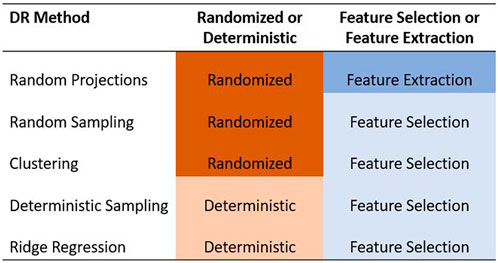
FIGURE 1. Summary of the five dimensionality reduction methods used in this paper. The methods are categorized as feature selection/feature extraction and as randomized/deterministic.
2.1 Random sketching
In order to understand the need for a random sketching algorithm, let us consider the simple example of linear regression. Suppose we have a X ∈ Rn×d full rank matrix of predictor variables and a response vector y of length n. The least squares estimates can be computed as,
Thus, we need the Gram matrix X′X and X′y to compute the solution. The computation of X′X requires O (nd2) time and X′y requires O (nd) time. When n > d, this solution is easy to calculate and is very popular in practice. But, when n, d or both are large—as they tend to be in many modern data sets—this computational time can be practically prohibitive.
Random sketching is a popular method to reduce the computational complexity of this problem. Instead of using the full data set (X, y), we can use a carefully constructed sketch
where
2.2 Random projection
Random projection algorithms form one of the major classes of random sketching algorithms. Random projection algorithms “uniformize” the non-uniformity structure present by rotating the matrix to a basis where the uniform random sampling of features is nearly optimal. Random projection can be viewed as the process of dimensionality reduction to preserve the pairwise distances between observations.
Random projection produces matrices formed by a small number of linear combinations of all of the original features. The linear combinations are formed by pre-multiplying the features with a randomly generated coefficients matrix, hence the name “random” projection. The resulting compressed matrix can be used as a substitute in computations, thereby reducing the computational complexity of the problem at hand. Given below is a simple random projection algorithm (Figure 2):
• Consider an input matrix A ∈ Rn×d with d ≫ n without loss of generality.
• Construct a d × k random projection matrix S, where k ≪ n.
• Obtain the sketched matrix B = AS, where B is a n × k matrix.
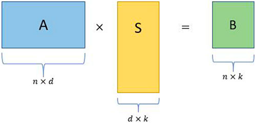
FIGURE 2. Schematic for a simple random projection where A is an input matrix, S is a random projection matrix, and B is the sketched matrix.
Let us consider the example of performing the Singular Value Decomposition (SVD) of A. Using the original matrix A, the exact computation of SVD takes O (nd2) time. Instead, if we settle for an approximate SVD of A, we can compute the SVD of B in place of A. The SVD computation on the smaller matrix B takes only O (nk2) time even with the simple algorithm presented above. This example illustrates the motivation for using random projection to reduce the dimensionality of large matrices.
Two questions come to mind quite naturally when looking at the above mentioned approach. How do we choose a suitable S to obtain good approximations? For what values of r will this algorithm produce good results? These two questions have been extensively studied over the last couple of decades and have led to several candidates for the projection matrix S and corresponding r values. We summarize some popular sketching matrices proposed in previous works:
• Gaussian Sketch: One of the first sketches proposed for random projection by Sarlos (2006). The sketch S was formed by sampling each element from a Gaussian distribution Sij ∼ N (0, 1/r), where Sij refers to the element in the ith row and jth column of matrix S.
• Rademacher Matrix: Achlioptas and Mcsherry (2007) proposed a simpler sketching matrix where each element of the matrix S is a random variable taking { + 1, −1} with equal probability. Further, they also proved that a sparse matrix with 2/3 of the entries replaced with 0 satisfies the Johnson-Lindenstrauss property. This modification was an important development, as the random matrix S becomes a sparse matrix and leads to faster computations.
• FJLT: Ailon and Chazelle (2009) came up with the concept of fast Johnson-Lindenstrauss transforms (FJLT). The sketching matrix was generated as a product of three matrices S = PHD, where P is a r × n sub-sampling matrix, H is a n × n dimension Hadamard matrix, and D is a n × n random diagonal matrix with entries taking values { + 1, −1} with equal probability. A Hadamard matrix is a square matrix with elements either { + 1, −1} and all the rows are orthogonal.
• CW Sketch: The Clarkson and Woodruff (2017) sketch is also a sparse matrix formed as a product of two independent random matrices S = ΓD, where Γ is a r × n random matrix with only one element of each column set to +1 and D is a n × n random diagonal matrix with entries taking values { + 1, −1} with equal probability. Thus, S will be a sparse random matrix with one non-zero entry in each of its columns.
If computing the lower-dimension projection was so computationally expensive that not much performance improvement was gained on the whole, the whole exercise becomes futile. Thus, there has been significant research into building projection mappings that will efficiently implement the random projection. Sparsification was a popular tool to reduce the number of computations performed during projection, as seen with the Rademacher matrix and FJLT approaches. In this paper, we used the FJLT method, also known as the subsampled randomized Hadamard transform (SRHT), to implement the random projection method as it supports fast computation and requires a modest amount of storage compared to other methods. Further details about the FJLT method can be found in the Supplementary Materials S1.
Like any feature extraction based DR method, the random projection method is based on the linear combinations of all the original features. The newly created features may not be interpretable in the data scale. Even worse, they may have no practical meaning at all. For this reason, feature selection is an attractive alternative approach to feature extraction as a means of dimensionality reduction. A subset of the original features is picked using various strategies in feature selection. This allows for a straightforward interpretation of results. In the next sections, we explore four feature selection algorithms, starting with the random sampling algorithm, the second approach to randomized sketching algorithms.
2.3 Random sampling
Random sampling is another randomized approach to forming lower-dimension approximation matrices. While random projection addresses the non-uniformity by “uniformizing” the structure through rotations, random sampling algorithms build an importance probability to address the non-uniformity. The random sampling approach involves sampling a small number of features that represent the whole set of features. Leverage scores can be interpreted as a measure of influence the data points have on related computations and hence can be viewed as a metric to define the non-uniformity in the original matrix. Given a matrix A ∈ Rn×d, let V′ denote the matrix containing the top right singular vectors of A. Then, the statistical leverage score of the ith column of A is defined as
The computational bottleneck for using the importance probability distribution lies in its dependence on the computation of the orthogonal basis for the original input matrix. Drineas et al. (2012) provided an algorithm to compute the relative-error approximate leverage scores li instead of computing the exact statistical leverage scores. Their contribution was a key development in the area of random sampling algorithms. We used their algorithm as the basis for implementing the random sampling algorithm in the genomic prediction problem.
We now describe the random sampling algorithm presented in Drineas et al. (2012) along with drawing the attention of the reader to the salient properties and contributions. Consider a matrix A ∈ Rn×d with d ≫ n and let V′ be the corresponding right singular matrix of A. Principally, we are interested in approximating the statistical leverage scores li of the columns of A, which are then used to construct the importance probability distribution.
where ei is the ith standard basis vector. The computation of the orthogonal matrix V′ takes O (n2d) time, which is the bottleneck. Since V′ can also be seen as any orthogonal basis for the column space of A, it follows that V′V = AA+ where + is the Moore-Penrose inverse. From this, we can redefine the statistical leverage scores as,
The computational complexity of calculating the leverage scores according to Eq. 2 involves computing the pseudo-inverse A+ and performing the matrix multiplication of A and A+. We apply random projection to overcome both these complexities by performing the computations and finally obtaining the approximate leverage scores
Instead of computing A+, we find a smaller matrix that approximates A and find the corresponding Moore-Pensore inverse of the smaller matrix. Subsampled Randomized Hadamard Transform (SRHT) is used to derive the smaller matrix as it preserves the structure A by rotating A to a random basis where all the rows have an equal influence and uniformly samples rows from that basis. If
While computing the product AA+ takes O (nd2), the computation of
Drineas et al. (2012) showed that for any error parameter ϵ ∈ (0, 0.5] and any arbitrary matrix A of size n × d with n ≫ d, the expression
holds for all i = 1, 2, … , n.
This result can be extended without loss of generality for d ≫ n case as well. Ma et al. (2015) investigated the approximation quality for several combinations of r1 and r2 through simulation studies. They found that r1 does not significantly impact the correlation between approximate and exact leverage scores but running time increases linearly with r1. On the other hand, the correlations between approximate and exact leverage scores increase rapidly with increasing r2, but r2 does not impact running time. Thus, they concluded that a combination of small r1 and large r2 would result in high-quality approximations with a short run time.
2.4 Deterministic sampling
Feature selection is also known as the column subset selection problem (CSSP) in matrix theory and linear algebra. Jolliffe (1972) proposed one of the first column subset selection algorithms. The algorithm involved deterministic sampling of the columns of the matrix based on ordered leverage scores. While the algorithm led to favorable dimensionality reduction in many practical applications, they did not provide theoretical guarantees on the quality of the approximation and hence it was not widely used for a long time. Drineas et al. (2008) developed the randomized counterpart to the deterministic sampling algorithm that employs a sampling probability distribution based on the leverage scores. They proved that their algorithm produces a matrix C that satisfies
The randomized algorithm gives a ‘near-optimal’ approximation of the matrix, but may not be computationally as efficient as the deterministic algorithm. Papailiopoulos et al. (2014) developed theoretical derivations for the approximation errors of the deterministic sampling algorithm provided by Jolliffe (1972). They proved that if the ordered leverage scores li follow a steep enough power-law decay, the deterministic algorithm performs equally or better than the randomized algorithm. Furthermore, suppose the leverage scores follow a steep power-law decay. In that case, the number of columns chosen by the deterministic algorithm is similar to or fewer than the randomized counterpart as proposed by Drineas et al. (2008). They showed the utility of the power-law decay assumption by providing several examples of real data sets where the leverage scores followed a power-law decay. Papailiopoulos et al. (2014) also emphasized that while their theoretical analysis was performed for the power-law decay model, other models for the leverage scores could be developed.
We now summarize the deterministic algorithm presented in Papailiopoulos et al. (2014). The deterministic algorithm can be described in three steps:
1. Compute the top-k right singular vectors Vk of A using SVD of A.
2. Calculate the leverage scores
3. Select c columns of A that correspond to the top c leverage scores such that their sum is greater than some stopping threshold θ,
The deterministic sampling algorithm requires the implementation of SVD to compute the leverage scores. Hence, the time complexity of the algorithm is given by O (nd min (n, d)). The resulting matrix from the deterministic sampling algorithm guarantees a bound on the approximation error with regard to the CSSP. Implementing the deterministic algorithm for the genomic prediction can be seen as a pre-processing step. Given a large genomic information matrix, we use the deterministic algorithm to create a compressed matrix that represents the whole matrix well.
The deterministic sampling algorithm implementation mimics the random sampling implementation with an ordered sampling approach instead of a randomized sampling, based on the leverage scores. In this work, we also evaluated clustering and penalized regression approaches for DR. Since these methods are well established and widely popular, we do not present them in great detail.
2.5 Clustering
Clustering is the process of grouping a set of objects in such a way that objects in the same group are more similar to each other than to objects in different groups, called clusters. Grouping objects when the data are labeled is a trivial task and is often referred to as supervised classification (Jain et al., 1999). But, often we are presented with data with no labeling available. Clustering was developed as a tool to deal with problems where the objective was to group unlabeled objects into meaningful collections. Because of the absence of labels, clustering is also called as unsupervised classification.
The general scheme of clustering is to start with n objects and sort them into K groups based on some similarity measure such that the intra-group similarity is high and the inter-group similarity is low. Several categorizations of the clustering algorithms are available, such as partitional and hierarchical algorithms.
Partitional clustering divides the set into non-overlapping subsets (clusters) such that each object is present only in one cluster. Typically, partitioning clusters produce clusters by optimizing some criterion function to produce optimal solutions (Hartigan, 1975). K-means, the most popular partitional algorithm, is an algorithm where the objective is to minimize the sum of the squares of the distances from the objects to the centroid of the cluster. K-means algorithm ensures that there are always exactly k clusters at the end of the process, with each cluster containing at least one item. While the algorithm is efficient and easy to implement, it is prone to issues such as the need for globular clusters and the need for uniform cluster sizes. The K-means algorithm and its shortcomings are presented in greater detail in the Supplementary Materials S1. Some of these drawbacks can be overcome by using a hierarchical clustering approach instead.
2.5.1 Hierarchical clustering algorithm
Hierarchical clustering is the process of creating a set of nested clusters arranged into a tree or dendrogram structure. Hierarchical clustering does not require a determination of the number of clusters k prior to the clustering process, as opposed to the k-means clustering. The nested structure provides flexibility of choosing the number of clusters based on the dendrogram as well as domain expertise (Jain et al., 1999). There are two possible directions of clustering under hierarchical clustering: agglomerative (bottom-up) and divisive (top-down). In this paper, we focus only on the agglomerative hierarchical clustering approach. The merging of clusters to form the hierarchy is determined by clustering metrics which define the similarity among the clusters. There are several clustering metrics available in the literature such as single-linkage, complete-linkage, average-linkage, and Ward’s method. We presented details about each of these clustering metrics in the Supplementary Materials S1.
Single-linkage is not the preferred metric due to its susceptibility to produce elongated clusters. Complete-linkage is avoided because of its inability to retain large clusters. Between average-linkage and Ward’s minimum variance method, there is no real distinguishing factor. Since Ward’s method can be compared easily to the objective function in k-means, we picked the Ward’s method as our metric of choice for the hierarchical clustering approach.
Hierarchical clustering creates a nested clustering structure, often represented by a dendrogram, which allows the user to create any number of clusters by choosing the appropriate height to cut the dendrogram. One of our objectives was to study the trend in prediction accuracy as a function of the input data sizes. Thus, we are interested in creating reduced data sets of different sizes. To obtain t data sets of different sizes, the K-means algorithm needs to be run t times. On the other hand, hierarchical clustering needs to be performed only once to determine the hierarchy. The t different sized marker data sets can then be created by cutting the dendrogram t times at appropriate heights.
2.6 Shrinkage methods
Variable selection is the process of choosing a subset of the explanatory variables to explain a response variable. Variable selection helps in making models easier to interpret, reducing noise introduced by redundant variables, and reducing the size of the data set for faster computations. When the number of variables is very large, traditional subset selection methods such as “best” subset selection are computationally infeasible. Step-wise selection methods were proposed as an alternative to reduce the computational load. A major drawback of the traditional and step-wise subset selection methods is the discrete nature of the variable selection, i.e., the variables are either retained or discarded. This leads to unstable variable selection, where a small change in data can lead to large change in the subset selected (Breiman, 1996).
Shrinkage methods were developed to address the shortcomings of the subset selection methods. These methods are also known as regularization or penalized methods. They work on the principle of imposing a constraint term that penalizes for model complexity. Shrinkage methods help in variable selection as well as improving the model’s prediction performance through the bias-variance trade-off. In other words, shrinkage methods may provide solutions that have lower variance and higher bias, but ultimately leading to better prediction accuracy according to the mean squared error (MSE).
In this paper, we investigate the shrinkage methods as a tool for variable selection. We use the coefficients of the predictors, obtained from the shrinkage methods, as a form of ranking of the variables for selection purposes.
Ridge regression uses all the d predictors in the final model. The algorithm shrinks all coefficients towards 0 through the L2 penalty, but does not set any of them exactly equal to zero. Hence, none of the predictors are removed from the final model. On the other hand, LASSO is a shrinkage method that applies an L1 penalty on the regression coefficients. Due to the nature of the L1 penalty, LASSO performs both shrinkage and automatic variable selection (Tibshirani, 1996). In other words, the penalty term not only shrinks the coefficients towards 0, it sets some of the coefficients to 0. When d > n, LASSO selects at most n variables (Zou and Hastie, 2005). Further, LASSO selects only one variable at random from a group of high correlated variables, often the case with genomic data. This can be a significant drawback in situations where selecting one of the variables from the group implies that all other variables are important as well because LASSO selects only one and discards the rest of the variables in the group.
Zou and Hastie (2005) proposed a new shrinkage method called the elastic net to overcome the problems presented by LASSO while retaining the advantages of LASSO. Elastic net can be viewed as a combination method involving both ridge regression and LASSO (Zou and Hastie, 2005). Elastic net allows for variable selection and also allows for group selection of variables, acting as an ideal combination of ridge regression and LASSO. It is appropriate for scenarios where d > n. We describe these three shrinkage methods - LASSO, ridge regression, and elastic net - along with their respective advantages and drawbacks in the supplementary section. Further details about the shrinkage methods can also be found in James et al. (2013).
The disadvantages presented by the LASSO algorithm, especially in context of genomic data makes it unsuitable for this study. Elastic net would be the ideal shrinkage algorithm for dimensionality reduction in practice. Unfortunately, it does not provide control on the number of variables selected in the final model. To answer all the objectives of the study, we needed fine control on the number of variables selected by each reduction method to help us compare the DR approaches to one another. Ridge regression performs shrinkage on the coefficients associated with the variables, but does not perform variable selection of any kind. Thus, we picked ridge regression as the shrinkage method of choice for this study.
In ridge regression, the penalty parameter has to be estimated separately. There are several methods for estimating the most appropriate penalty parameter λ. The most popular and reliable method is cross-validation. We can choose a range of λ values, compute the cross-validated error for each value of λ and pick the λ corresponding to the smallest cross-validation error (James et al., 2013).
3 Implementation of methods
In this paper, we used five different DR methods as pre-processing step to genomic prediction models. We implemented the methods to reduce the dimensionality of the genomic data to help reduce the computational resource requirements such as memory, storage, and time. In this section, we present details about the implementation of each of the five DR methods on the genomic data to create data sets of differing sizes to evaluate the trends in prediction as the function of the dimensionality.
3.1 Implementation of the random projection algorithm
We used the RaProR package (Geppert et al., 2019) in R (R Core Team, 2020) to compute the random projection. The package was built based on theorems and results in Geppert et al. (2017), which provides details about the algorithms implemented to compute the projection. We used the SRHT projection for our random projection implementation in this study. The implementation of the random projection algorithm for dimensionality reduction of the genomic marker data set can be visualized in Figure 3 and can be summarized as follows:
1. Compute projection matrices with a predefined number of columns k.
2. Multiply the projection matrix with original marker data to obtain the reduced matrix X of size n × k.
3. Use the reduced matrix to compute the genetic relationship matrix as G = XX′/d, where G denotes the genetic relationship matrix, as the input for genomic prediction models and obtain predictions in different cross-validation schemes (described in Sections 4.1 and 4.2). The genetic relationship matrix describes the relationship between individuals, and captures the population structure.
4. Repeat steps 2–4 100 times to remove bias in the prediction results.
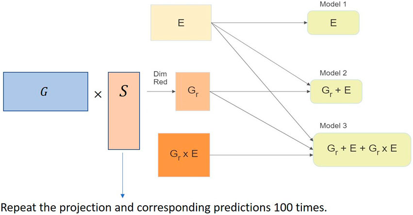
FIGURE 3. Implementation of the random projection algorithm for dimensionality reduction of the genomic data set in the genomic prediction problem.
3.2 Implementation of the random sampling algorithm
We used the statistical leverage scores to calculate the importance probability distribution required for the random sampling algorithm. We followed the two-stage algorithm presented by Boutsidis et al. (2009) to implement the random sampling algorithm. The implementation of the random sampling algorithm for dimensionality reduction of the marker data set for genomic prediction is as follows:
1. Compute the approximate leverage scores as defined in Drineas et al. (2012).
2. Use the approximate leverage scores to define the importance sampling distribution for the columns of the input marker matrix X.
3. Randomly sample a predefined number of columns k according to the importance sampling distribution to form reduced matrices of different sizes.
4. Use the reduced matrix X to compute the genetic relationship matrix G = XX′/d as the input for the prediction models and obtain predictions in different cross-validation schemes (described in Sections 4.1 and 4.2).
5. Repeat steps 3–4 100 times to remove sampling bias from the prediction accuracy results.
The advantage of this random sampling algorithm is the computation of the approximate leverage scores instead of the exact scores, effectively reducing computation time.
3.3 Implementation of clustering for dimensionality reduction
This section describes our approach to applying dimensionality reduction to genomic data sets using clustering. The R package “fastcluster” (Müllner, 2013) was used for fast implementation of the hierarchical clustering algorithm. Once the dendrogram was created, the cuts were made to form the k clusters. The cut height is determined by the R package to ensure that the user-defined k number of clusters are created. The implementation of the clustering algorithm for dimensionality reduction of the genomic data set can be summarized as follows:
1. Perform agglomerative hierarchical clustering using “fastcluster” to determine the hierarchy.
2. Form k clusters from the hierarchy by cutting appropriately.
3. Sample one feature randomly from each of the k clusters as the representative of that cluster.
4. The sampled features form the reduced data set of size k and will be used for the genomic prediction models.
5. Repeat the sampling from the clusters and the following model implementation 100 times to remove sampling bias in the prediction accuracy results.
3.4 Implementation of the deterministic sampling algorithm
The deterministic sampling algorithm implementation mimics the random sampling implementation without the randomized sampling based on the leverage scores. The deterministic sampling algorithm can be summarized as follows:
1. Compute the approximate leverage scores as defined in Drineas et al. (2012).
2. Arrange the leverage scores in decreasing order.
3. Pick the top k leverage scored columns to form the reduced matrices.
4. Use these reduced matrices as the input for the genomic prediction models.
3.5 Implementation of ridge regression for dimensionality reduction
We used the “glmnet” (Simon et al., 2011) package in R to implement ridge regression. Given below is the implementation of the ridge regression algorithm for dimensionality reduction of the genomic data set for genomic prediction:
1. Implement a ridge regression model with the standardized features corresponding to the marker information.
2. Use the coefficients estimated from the ridge regression as a measure of importance of the features.
3. Order the features by their respective regression coefficients.
4. Pick the top k features to form the reduced data set for the genomic prediction models.
4 Data and genomic prediction models
All the methods were applied to a chickpea data set collected by the International Chickpea Screening Nursery (ICSN) of ICRISAT (Roorkiwal et al., 2016). The lines were phenotyped for three seasons (2012–13, 2013–14, and 2014–15) at two locations (ICRISAT, Patancheru and IARI, New Delhi) under different water regimes (normal-rainfed, irrigated, or late-sown), which resulted in nine environments (unique season-location-water combinations). Phenotypic data on eight traits were collected: 100 Seed Weight (100-SDW measured in grams), Biomass (BM measured in grams), Days to 50% Flowering (DF measured number of days), Days to Maturity (DM measured in number of days), Harvest Index (HI measured in %), Plant Height (PH measured in centimeters), Number of Plant Stand (PS measured in number of plants) and Seed Yield (SY measured in grams). Since one of the most important trait for plant breeders is yield, in this paper, we evaluated the DR methods with the seed yield (SY) as the phenotype of interest. The calculations can be performed the same way for the other traits.
The original data set contained 315 lines phenotyped in nine environments, giving a total of 2,835 phenotypic yield observations. All of the 315 lines had corresponding genomic data with 26,817 markers each. After cleaning the data as described in the Supplementary Materials S1, the genomic data had 306 observations and 14,928 features, which could be viewed as a matrix of size 306 × 14,928. In the following section, we describe the models used for genomic prediction as well as the techniques used to evaluate the accuracy of the models.
4.1 Prediction models
In this work, we used the models proposed by Jarquín et al. (2014) to evaluate the predictive ability of reduced datasets. Specifically, we considered three models based on the input information in each model: either environmental and line information (E + L) only, or genomic information along with environment information (G + E), or genomic information with environmental information as well as their interactions (G + E + G×E) as the predictors.
Let the phenotypic trait be represented by yijk for the kth replicate for the jth line in the ith environment. Let the environmental effect be represented by Ei (i = 1, 2, … , I), the line effect be defined by Lj (j = 1, 2, …, J), the genetic effect be denoted by gj (j = 1, 2, …, J), the interaction be denoted by gEij and the error term be represented as ϵijk (k = 1, 2, …, rij). The three models corresponding to the three scenarios mentioned above are given by:
where μ is the overall mean,
Using the dimensionality reduction methods, we reduce the size of the marker matrix (X) and thus the dimensionality reduction methods affect only the G + E (Eq. 7) and G + E + G × E (Eq. 8) models but not the baseline E + L model (Eq. 6).
4.2 Model assessment using cross-validation schemes
Three different cross-validation schemes were implemented to assess the predictive ability of the models in different scenarios. These are scenarios that breeders might be interested in since these mimic the situations they face in their breeding programs. The performance of the prediction models was assessed by measuring the Pearson correlations (Waldmann, 2019) between the observed phenotypic values and the predicted genomic estimated breeding values within environments. The three different cross-validations can be summarized as the prediction of lines in a new unobserved environment (CV0), the prediction of new untested lines in environments (CV1), and the prediction of lines that were observed in some environments but not observed in other environments (CV2).
CV0 refers to the cross-validation that evaluates the ability of the models to predict the performance of lines in a new unobserved environment. In effect, we performed a k-fold cross-validation in which we left out the observations from the observed target environment in each fold and used the other observations from the other (k − 1) environments as the training set. We computed the correlations between the observed and predicted values within each environment. This correlation quantified a model’s ability to predict the performance of all the lines in a new environment.
CV1 refers to the cross-validation that evaluates the ability of the models to predict the performance of untested lines in all environments. For CV1 a five-fold cross-validation scheme was used where we randomly selected 20% of the lines as the testing group and left out all the observations corresponding to these lines from all environments. We used the observations from the other 80% of the lines as the training set to build the prediction models. Then, we predicted the trait values for the lines left out across all environments. This process of creating folds randomly and performing predictions was repeated 20 times. Finally, we computed the correlations between the observed and predicted values within each environment and averaged them across the 20 runs to obtain the average correlations.
CV2 refers to the cross-validation that evaluates the ability of the models to predict the performance of lines that were tested in some environments but not tested in other environments. For CV2, the phenotypic observations were randomly partitioned into five subsets without regard for the lines or environment. Four subsets were combined and used for training the models, and the remaining subset was used as a test set. The process was repeated 20 times, just as described in CV1, to obtain average correlations.
5 Dimensionality reduction in genomic prediction
We investigated five DR methods in this paper. We performed feature selection or feature extraction for each method to create reduced dimensional marker data sets of 26 different sizes based on the number of markers present. The number of markers ranged from 200 to 14,928 (the full marker data set). We set the number of markers as fixed across all methods to compare the dimensionality reduction methods and their prediction ability at each size. For the three randomized dimensionality reduction methods, 100 data sets were generated at each size, and prediction results from the 100 data sets were averaged and set as the prediction accuracy of that size. This was done to overcome any bias that the random selection process may have introduced. For each reduced data set, we implemented the three predictions models (Eqs 6–8) and evaluated each model using the three cross-validation schemes described in the previous section. CV1 and CV2 cross-validation schemes were run 20 times on each set due to the randomization introduced during the fold creation. Taking into consideration all the different methods, sizes, randomization, prediction models, and cross-validation schemes, we ran over 965,000 combinations in this study.
6 Results
This study focused on two objectives. The primary objective was to evaluate the merit of using dimensionality reduction methods as a pre-processing step in genomic prediction. We used five dimensionality reduction methods to present dimensionality reduction as an effective pre-processing step in genomic prediction. We compared their reduction capabilities to find which methods work better for genomic prediction across different prediction models and cross-validation schemes. Second, we studied the trends in prediction accuracy of reduced data sets as a function of their size.
The results from these models are summarized in the plots in Figures 4, 5. For each model and cross-validation combination, the correlation results for the full unreduced SNP data are referenced using a grey horizontal line.
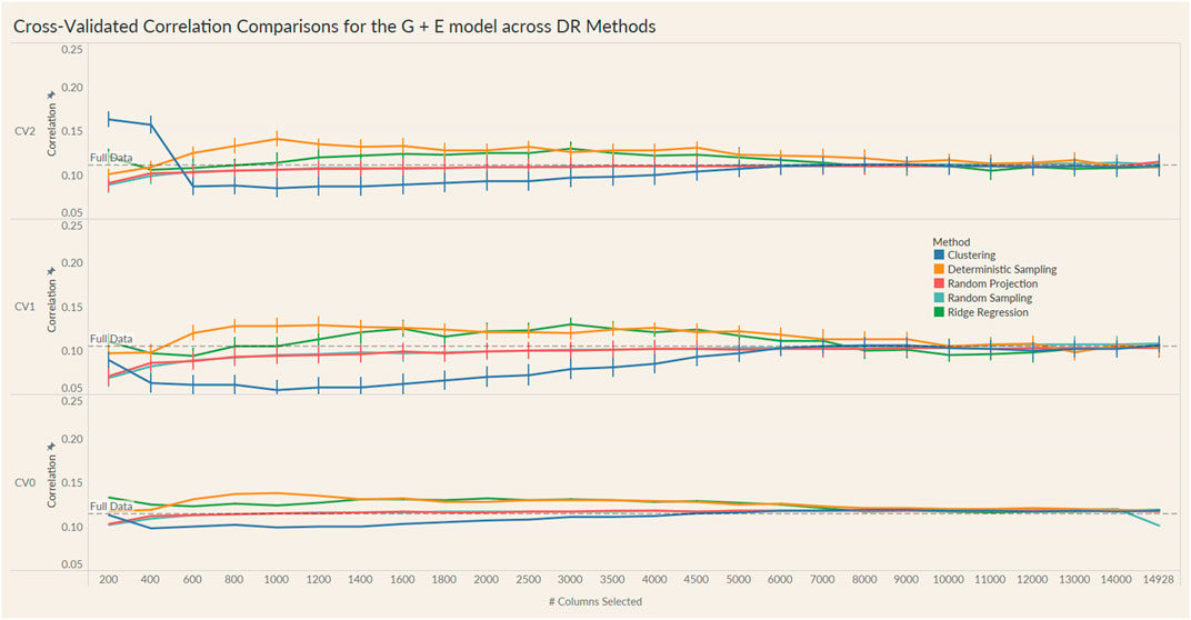
FIGURE 4. Prediction accuracy for the seed yield trait of a chickpea population consisting of 306 genotypes tested in nine environments for the G + E model under the three cross-validation schemes (CV0, CV1, CV2) across 26 different genomic information sizes. Standard errors are depicted at each size.
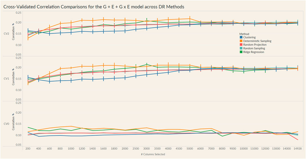
FIGURE 5. Prediction accuracy for the seed yield trait of a chickpea population consisting of 306 genotypes tested in nine environments for the G + E + GxE model under the three cross-validation schemes (CV0, CV1, CV2) across 26 different genomic information sizes. Standard errors are depicted at each size.
Irrespective of the model and CV scheme, all dimensionality reduction methods required only a fraction of the total input markers to obtain maximum correlation. In addition, we observed a plateauing of correlation values as the number of markers selected increased for all methods. Thus, the number of markers required to achieve maximum correlation may be an inappropriate measure to evaluate the reduction capability of the method. Instead, we considered a 95% of the maximum correlation as our metric to evaluate the reduction methods. For instance, for the CV1 scheme in the G × E model, the random projection algorithm achieved the maximum correlation of 0.195 with all 14,928 input markers. However, the method achieved a 95% maximum correlation of 0.185 with just 3,000 input markers. This significantly reduces the number of input markers for similar correlation values. In fact, for all the dimensionality reduction methods, fewer than 40% of the input markers were required to achieve a 95% max correlation value. These results are summarized in Table 1. Furthermore, for the deterministic sampling and ridge regression based reduction, the highest correlation was achieved by a reduced data set rather than using the whole data set in all three models, indicating the presence of noise in the data.
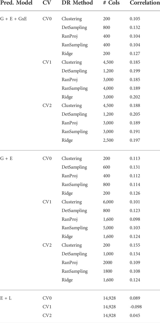
TABLE 1. Number of markers selected by each dimensionality reduction (DR) method to obtain 95% of the highest correlation for the three prediction models (G + E + GxE, G + E, E + L) under the three cross-validation schemes (CV0, CV1, CV2).
Second, no one reduction method had the best reduction capability across all prediction models and CV combinations. For instance, for the CV2 scheme of the G × E model, deterministic sampling required only 1,200 markers in the input data to achieve 95% of the maximum correlation compared to the 4,500 required by clustering. On the other hand, for the CV2 scheme of the G + E model, clustering required only 200 input markers to attain 95% of the maximum correlation compared to the 1,000 required by deterministic sampling. Random projection and random sampling methods were very similar in terms of prediction accuracy values across all matrix sizes by model by cross-validation combinations. All the reduction methods had similar prediction accuracies within the model and CV combination, which reiterates the utility of dimensionality reduction regardless of the DR method used.
7 Discussion
Modern plant breeding programs combine genomic information with phenotypic performance data to select favorable lines. Early genomic selection models included the line, environment, phenotypic and genomic information to predict the performance of lines. Genetic information, environmental factors, and their interactions affect complex traits such as yield. Hence, the development of models that allowed for this genotype by environment interactions improved the genomic prediction accuracy. The improvements in genotyping technology combined with the reducing cost have led to the generation of genomic data of enormous sizes that are often high-dimensional. While current genomic selection models can handle these high-dimensional data, there are questions about their efficiency. Further, including information on hundreds of thousands of potentially unrelated markers in the genomic prediction models could negatively impact the prediction accuracy of the trait of interest. Lastly, there is a computational resource cost that must be taken into account. Prediction models with larger input sizes require much greater computational resources to run, both in terms of hardware and time. We proposed dimensionality reduction as a mechanism to address all of these concerns.
In this study, we used a chickpea data set. Chickpea is the second largest produced food legume crop in the world (Roorkiwal et al., 2016). Its high protein content makes it a valuable source of protein in several cultures worldwide, especially in vegetarian diets. Implementation of GS methods helps breeding programs reduce breeding cycle time and improve the rate of genetic gains (Roorkiwal et al., 2018) by allowing breeders to select lines using genomic marker data before performing field trials. With the recent improvements in the high-throughput genotyping technologies, millions of markers are available for several hundred chickpea lines. GS has been adept at accessing these large data sets to predict the performance of lines. However, further advances in this area will yield larger marker data sets, which could overwhelm the current GS methods and the available computational resources. In addition, other high-dimensional data such as high-dimensional weather covariates and high-throughput phenotyping information are increasingly more available in breeding programs. While we did not consider such data in this study, the inclusion of such data could create computational bottlenecks. These reasons present a need to develop methods that effectively handle large data sets and use the additional data available to improve prediction accuracy.
The key contribution of this work was to propose using dimensionality reduction in genomic prediction analyses and show its utility using a hand-picked subset of all available methods. For example, we explored the possibility of using randomized algorithms for dimensionality reduction with the help of primitive implementations. Several more sophisticated randomized algorithms could improve dimensionality reduction, which can be explored in future works. Our results act as a proof of concept that future researchers can use to explore various dimensionality reduction methods and identify the best method for their breeding data. Our results clearly indicate the need to integrate dimensionality reduction methods into genomic selection to reduce computational resource requirements, improve the prediction process, and select the best performing lines in any breeding program.
Data availability statement
The original contributions presented in the study are included in the article/Supplementary Material, further inquiries can be directed to the corresponding author.
Author contributions
VM, RV, DJ, and RH contributed to the conception and design of the study. RV designed and executed the field and genotyping experiments. VM wrote the code for the methods and prediction models. VM, DJ, and RH were responsible for interpretation of the results. VM wrote the first draft of the manuscript. DJ and RH contributed to revisions. All authors edited, reviewed, and approved the submitted version.
Funding
VM was partially supported by the Development of Waxy Sorghum Lines Grant from the Department of Agriculture - NIFA (UNR 19-58). DJ was supported by the Agriculture and Food Research Initiative Grant (NEB-21-176) from the USDA National Institute of Food and Agriculture, Plant Health and Production and Plant Products: Plant Breeding for Agricultural Production, A1211, Accession No. 1015252.
Acknowledgments
This research was done using resources provided by the Open Science Grid (Pordes et al., 2007; Sfiligoi et al., 2009), which is supported by the National Science Foundation award #2030508. This work was completed utilizing the Holland Computing Center of the University of Nebraska, which receives support from the Nebraska Research Initiative.
Conflict of interest
The authors declare that the research was conducted in the absence of any commercial or financial relationships that could be construed as a potential conflict of interest.
Publisher’s note
All claims expressed in this article are solely those of the authors and do not necessarily represent those of their affiliated organizations, or those of the publisher, the editors and the reviewers. Any product that may be evaluated in this article, or claim that may be made by its manufacturer, is not guaranteed or endorsed by the publisher.
Supplementary material
The Supplementary Material for this article can be found online at: https://www.frontiersin.org/articles/10.3389/fgene.2022.958780/full#supplementary-material
References
Achlioptas, D., and Mcsherry, F. (2007). Fast computation of low-rank matrix approximations. J. ACM 54, 9. doi:10.1145/1219092.1219097
Ailon, N., and Chazelle, B. (2009). The fast johnson–lindenstrauss transform and approximate nearest neighbors. SIAM J. Comput. 39, 302–322. doi:10.1137/060673096
Boutsidis, C., Mahoney, M. W., and Drineas, P. (2009). “An improved approximation algorithm for the column subset selection problem,” in Proceedings of the Twentieth Annual ACM-SIAM Symposium on Discrete Algorithms, New york, Jan 4-6, 968–977. (USA: Society for Industrial and Applied Mathematics). doi:10.1137/1.9781611973068.105
Breiman, L. (1996). Heuristics of instability and stabilization in model selection. Ann. Statistics 24, 2350–2383. Publisher: Institute of Mathematical Statistics. doi:10.1214/aos/1032181158
Burgueño, J., Campos, G. d. l., Weigel, K., and Crossa, J. (2012). Genomic prediction of breeding values when modeling genotype × environment interaction using pedigree and dense molecular markers. Crop Sci. 52, 707–719. doi:10.2135/cropsci2011.06.0299
Burgueño, J., Crossa, J., Cornelius, P. L., and Yang, R.-C. (2008). Using factor Analytic models for joining environments and genotypes without crossover genotype × environment interaction. Crop Sci. 48, 1291–1305. doi:10.2135/cropsci2007.11.0632
Burgueño, J., Crossa, J., Cotes, J. M., Vicente, F. S., and Das, B. (2011). Prediction assessment of linear mixed models for multienvironment trials. Crop Sci. 51, 944–954. doi:10.2135/cropsci2010.07.0403
Clarkson, K. L., and Woodruff, D. P. (2017). Low-rank approximation and regression in input sparsity time. J. ACM 63, 1–45. doi:10.1145/3019134
Crossa, J., Burgueño, J., Cornelius, P. L., McLaren, G., Trethowan, R., and Krishnamachari, A. (2006). Modeling genotype × environment interaction using additive genetic covariances of relatives for predicting breeding values of wheat genotypes. Crop Sci. 46, 1722–1733. doi:10.2135/cropsci2005.11-0427
Crossa, J., Yang, R.-C., and Cornelius, P. L. (2004). Studying crossover genotype × environment interaction using linear-bilinear models and mixed models. J. Agric. Biol. Environ. Stat. 9, 362–380. doi:10.1198/108571104X4423
De los Campos, G., Gianola, D., Rosa, G. J. M., Weigel, K. A., and Crossa, J. (2010). Semi-parametric genomic-enabled prediction of genetic values using reproducing kernel Hilbert spaces methods. Genet. Res. 92, 295–308. doi:10.1017/S0016672310000285
de los Campos, G., Naya, H., Gianola, D., Crossa, J., Legarra, A., Manfredi, E., et al. (2009). Predicting quantitative traits with regression models for dense molecular markers and pedigree. Genetics 182, 375–385. doi:10.1534/genetics.109.101501
Deshpande, A., Rademacher, L., Vempala, S., and Wang, G. (2006). Matrix approximation and projective clustering via volume sampling. ToC. 2, 225–247. doi:10.4086/toc.2006.v002a012
Drineas, P., Kannan, R., and Mahoney, M. W. (2006a). Fast Monte Carlo algorithms for matrices II: Computing a low-rank approximation to a matrix. SIAM J. Comput. 36, 158–183. doi:10.1137/S0097539704442696
Drineas, P., Magdon-Ismail, M., Mahoney, M. W., and Woodruff, D. P. (2012). Fast approximation of matrix coherence and statistical leverage. J. Mach. Learn. Res. 13, 3475–3506. doi:10.5555/2503308.2503352
Drineas, P., Mahoney, M. W., and Muthukrishnan, S. (2008). Relative-error $CUR$ matrix decompositions. SIAM J. Matrix Anal. Appl. 30, 844–881. doi:10.1137/07070471X
Drineas, P., Mahoney, M. W., and Muthukrishnan, S. (2006b). “Sampling algorithms for l2 regression and applications,” in SODA ’06: Proceedings of the seventeenth annual ACM-SIAM symposium on Discrete algorithm, Miami, Florida, Jan 22-24, 1127–1136. (USA: Society for Industrial and Applied Mathematics).
Drineas, P., Mahoney, M. W., Muthukrishnan, S., and Sarlós, T. (2011). Faster least squares approximation. Numer. Math. (Heidelb). 117, 219–249. doi:10.1007/s00211-010-0331-6
Drineas, P., and Zouzias, A. (2011). A note on element-wise matrix sparsification via a matrix-valued Bernstein inequality. Inf. Process. Lett. 111, 385–389. doi:10.1016/j.ipl.2011.01.010
Eckart, C., and Young, G. (1936). The approximation of one matrix by another of lower rank. Psychometrika 1, 211–218. doi:10.1007/BF02288367
Fisher, R. A. (1936). The use of multiple measurements in taxonomic problems. Ann. Eugen. 7, 179–188. doi:10.1111/j.1469-1809.1936.tb02137.x
Frieze, A., Kannan, R., and Vempala, S. (2004). Fast monte-carlo algorithms for finding low-rank approximations. J. ACM 51, 1025–1041. doi:10.1145/1039488.1039494
Geppert, L. N., Ickstadt, K., Munteanu, A., Quedenfeld, J., Sandig, L., and Sohler, C. (2019). RaProR: Calculate sketches using random projections to reduce large data sets. R package version 1, 1–5.
Geppert, L. N., Ickstadt, K., Munteanu, A., Quedenfeld, J., and Sohler, C. (2017). Random projections for Bayesian regression. Stat. Comput. 27, 79–101. doi:10.1007/s11222-015-9608-z
Ghashami, M., Liberty, E., Phillips, J. M., and Woodruff, D. P. (2015). Frequent directions : Simple and deterministic matrix sketching. arXiv:1501.01711 [cs] ArXiv: 1501.01711 Comment: 28 pages , This paper contains Frequent Directions algorithm (see arXiv:1206.0594) and relative error bound on it (see arXiv:1307.7454).
Gianola, D., Fernando, R. L., and Stella, A. (2006). Genomic-assisted prediction of genetic value with semiparametric procedures. Genetics 173, 1761–1776. doi:10.1534/genetics.105.049510
Golub, G. H., and Van Loan, C. F. (2013). “Matrix computations,” in Johns Hopkins studies in the mathematical sciences. fourth edition edn (Baltimore: The Johns Hopkins University Press). OCLC: ocn824733531.
Heslot, N., Yang, H.-P., Sorrells, M. E., and Jannink, J.-L. (2012). Genomic selection in plant breeding: A comparison of models. Crop Sci. 52, 146–160. doi:10.2135/cropsci2011.06.0297
Hoerl, A. E., and Kennard, R. W. (1970). Ridge Regression: Biased estimation for nonorthogonal problems. Technometrics 12, 55–67. doi:10.1080/00401706.1970.10488634
Jain, A. K., Murty, M. N., and Flynn, P. J. (1999). Data clustering: a review. ACM Comput. Surv. 31, 264–323. doi:10.1145/331499.331504
James, G., Witten, D., Hastie, T., and Tibshirani, R. (2013). An Introduction to statistical learning, 103. New York, NY: Springer New York. doi:10.1007/978-1-4614-7138-7
Jarquín, D., Crossa, J., Lacaze, X., Du Cheyron, P., Daucourt, J., Lorgeou, J., et al. (2014). A reaction norm model for genomic selection using high-dimensional genomic and environmental data. Theor. Appl. Genet. 127, 595–607. doi:10.1007/s00122-013-2243-1
Jarquín, D., Lemes da Silva, C., Gaynor, R. C., Poland, J., Fritz, A., Howard, R., et al. (2017). Increasing genomic-enabled prediction accuracy by modeling genotype × environment interactions in Kansas wheat. Plant Genome 10. doi:10.3835/plantgenome2016.12.0130
Johnson, W., and Lindenstrauss, J. (1984). Extensions of lipschitz mappings into a Hilbert space. Contemp. Math. 26, 189–206. doi:10.1090/conm/026/737400
Jolliffe, I. T. (1972). Discarding variables in a principal component analysis. I: Artificial data. J. R. Stat. Soc. Ser. C Appl. Statistics) 21, 160–173. Publisher: [Wiley, Royal Statistical Society]. doi:10.2307/2346488
Liberty, E., Woolfe, F., Martinsson, P.-G., Rokhlin, V., and Tygert, M. (2007). Randomized algorithms for the low-rank approximation of matrices. Proc. Natl. Acad. Sci. U. S. A. 104, 20167–20172. doi:10.1073/pnas.0709640104
Long, N., Gianola, D., Rosa, G. J. M., and Weigel, K. A. (2011). Application of support vector regression to genome-assisted prediction of quantitative traits. Theor. Appl. Genet. 123, 1065–1074. doi:10.1007/s00122-011-1648-y
Ma, P., Mahoney, M. W., and Yu, B. (2015). A statistical perspective on algorithmic leveraging. J. Mach. Learn. Res. 16, 861–911. doi:10.48550/arXiv.1306.5362
Mahoney, M. W., and Drineas, P. (2009). CUR matrix decompositions for improved data analysis. Proc. Natl. Acad. Sci. U. S. A. 106, 697–702. doi:10.1073/pnas.0803205106
Meuwissen, T. H., Hayes, B. J., and Goddard, M. E. (2001). Prediction of total genetic value using genome-wide dense marker maps. Genetics 157, 1819–1829. doi:10.1093/genetics/157.4.1819
Moser, G., Tier, B., Crump, R. E., Khatkar, M. S., and Raadsma, H. W. (2009). A comparison of five methods to predict genomic breeding values of dairy bulls from genome-wide SNP markers. Genet. Sel. Evol. 41, 56. doi:10.1186/1297-9686-41-56
Müllner, D. (2013). Fastcluster : Fast hierarchical, agglomerative clustering routines for R and Python. J. Stat. Softw. 53. doi:10.18637/jss.v053.i09
Musco, C. N. C. N. (2018). The power of randomized algorithms : from numerical linear algebra to biological systems. Thesis, Massachusetts Institute of Technology (Accepted: 2019-02-14T15:50:19Z ISBN: 9781084478763 Journal Abbreviation: From numerical linear algebra to biological systems.
Papailiopoulos, D., Kyrillidis, A., and Boutsidis, C. (2014). Provable deterministic leverage score sampling. arXiv:1404.1530 [cs, math, stat] ArXiv: 1404.1530.
Pearson, K. (1901). Liii. on lines and planes of closest fit to systems of points in space. Lond. Edinb. Dublin Philosophical Mag. J. Sci. 2, 559–572. doi:10.1080/14786440109462720
Pordes, R., Petravick, D., Kramer, B., Olson, D., Livny, M., Roy, A., et al. (2007). The open science grid. J. Phys. Conf. Ser. 78, 012057. doi:10.1088/1742-6596/78/1/012057
R Core Team (2020). R: A language and environment for statistical computing. Vienna, Austria: R Foundation for Statistical Computing.
Roorkiwal, M., Jarquin, D., Singh, M. K., Gaur, P. M., Bharadwaj, C., Rathore, A., et al. (2018). Genomic-enabled prediction models using multi-environment trials to estimate the effect of genotype × environment interaction on prediction accuracy in chickpea. Sci. Rep. 8, 11701. doi:10.1038/s41598-018-30027-2
Roorkiwal, M., Rathore, A., Das, R. R., Singh, M. K., Jain, A., Srinivasan, S., et al. (2016). Genome-Enabled prediction models for yield related traits in chickpea. Front. Plant Sci. 7. Publisher: Frontiers. doi:10.3389/fpls.2016.01666
Sarlos, T. (2006). “Improved approximation algorithms for large matrices via random projections,” in 2006 47th Annual IEEE Symposium on Foundations of Computer Science (FOCS’06), Berkeley, CA, Oct 21-24, 143–152. (IEEE). doi:10.1109/FOCS.2006.37
Sfiligoi, I., Bradley, D. C., Holzman, B., Mhashilkar, P., Padhi, S., and Wurthwein, F. (2009). The pilot way to grid resources using glideinwms. WRI World Congr. Comput. Sci. Inf. Eng. 2, 428–432. doi:10.1109/CSIE.2009.950
Simon, N., Friedman, J., Hastie, T., and Tibshirani, R. (2011). Regularization paths for cox’s proportional hazards model via coordinate descent. J. Stat. Softw. 39, 1–13. doi:10.18637/jss.v039.i05
Sneath, P. H. A., and Sokal, R. R. (1973). “Numerical taxonomy,” in The principles and practice of numerical classification. 1st Edn. San Francisco: W. H. Freeman.
Tibshirani, R. (1996). Regression shrinkage and selection via the lasso. J. R. Stat. Soc. Ser. B 58, 267–288. doi:10.1111/j.2517-6161.1996.tb02080.x
Tropp, J. A., Yurtsever, A., Udell, M., and Cevher, V. (2017). Practical sketching algorithms for low-rank matrix approximation. SIAM J. Matrix Anal. Appl.Society Industrial Appl. Math. 38, 1454–1485. doi:10.1137/17m1111590
Usai, M. G., Sardegna, A., Profile, S., Usai, M. G., Goddard, M. E., and Hayes, B. J. (2009). LASSO with cross-validation for genomic selection. Genet. Res. 91 (6), 427. doi:10.1017/S0016672309990334
Waldmann, P. (2019). On the use of the pearson correlation coefficient for model evaluation in genome-wide prediction. Front. Genet. 10, 899. doi:10.3389/fgene.2019.00899
Keywords: dimensionality reduction, chickpea, genomic selection, randomized algorithms, genomic prediction
Citation: Manthena V, Jarquín D, Varshney RK, Roorkiwal M, Dixit GP, Bharadwaj C and Howard R (2022) Evaluating dimensionality reduction for genomic prediction. Front. Genet. 13:958780. doi: 10.3389/fgene.2022.958780
Received: 01 June 2022; Accepted: 05 September 2022;
Published: 14 October 2022.
Edited by:
Zitong Li, Commonwealth Scientific and Industrial Research Organisation (CSIRO), AustraliaReviewed by:
Pierce Rafter, Teagasc, IrelandAlan Cleary, National Center for Genome Resources, United States
Copyright © 2022 Manthena, Jarquín, Varshney, Roorkiwal, Dixit, Bharadwaj and Howard. This is an open-access article distributed under the terms of the Creative Commons Attribution License (CC BY). The use, distribution or reproduction in other forums is permitted, provided the original author(s) and the copyright owner(s) are credited and that the original publication in this journal is cited, in accordance with accepted academic practice. No use, distribution or reproduction is permitted which does not comply with these terms.
*Correspondence: Reka Howard, rekahoward@unl.edu