Evidence regarding the ecological benefits of payment for ecological services programs from China’s grassland ecological compensation policy

1 Introduction

Natural resources over-exploitation is a rising concern. Policy makers around the world are turning to payments for ecosystem services programs in an effort to deal with this issue (Kleijn and Sutherland, 2003; Cao et al., 2009; Wu and Lin, 2010; Whittingham, 2011; Deng et al., 2012; Chen et al., 2015; Börner et al., 2017; Sims and Alix-Garcia, 2017; Ding and Yao, 2021; Hayes et al., 2022). However, the ecological benefits of paying for ecosystem services programs are still unclear. In this study, our aim is to assess whether payment for ecosystem services programs would bring substantial ecological benefits by focusing on China’s grassland ecological compensation policy (GECP)—the planet’s largest.

We assembled a panel of counties across China to assess the impact on grassland quality of the GECP over the decade 2005–2015. The evidence suggests that policy leads to an increase in grassland quality and that its average impact is economically and statistically significant. Our estimates imply that counties which go from not launching the GECP to launching it achieve on average 4% larger grassland quality in following years than counties that do not.

To understand whether the impact on grassland quality of the GECP was evenly distributed across different regions, we examined evidence from heterogeneity analysis. We found that the GECP’s impact on grassland quality was dependent on county characteristics. That is, the GECP would be more conductive to increasing in grassland quality for counties which are warmer, richer, and have lower population densities.

Finally, in order to demonstrate the robustness of our results, we implemented a series of sensitivity analyses, including the leave-one-county-out-test, bootstrapping test, and permutation test. The results of the three tests also suggested that the GECP has an economically and statistically significant positive impact on grassland quality.

There is little extant literature in the environmental sciences that investigates the ecological benefits of payment for ecosystem services programs (Hu et al., 2019). In a case study, Liu et al. (2018) evaluated the impact of Inner Mongolia’s grassland quality on China’s GECP, producing a positive though little credited result. We also build on and complement Hou et al. (2021), who also employed a difference-in-differences estimator. Using this approach, they assessed the impact of China’s GECP on pilot regional grassland quality. Unlike us, they did not control regional social and economic characteristics, although they absorbed weather conditions. Besides differences in control and specification, our estimation strategy differs from Hou et al. (2021)in that we additionally adopt a matching framework by balancing the propensity to launch the GECP between the treated group and the control group, which produces a more credible estimate of the impact than their estimator.

The rest of this article is organized as follows. The next section describes the construction of the dataset and the implementation of the models, which are used in later empirical analysis. Section 3 presents the estimates from our three estimators, including the difference-in-differences estimator, the propensity-score-matching difference-in-differences estimator, and the inverse-probability-weighting difference-in-differences estimators. In that section, we also examine whether the treated group and the control group were comparable, report the results from heterogeneity analysis, and carry out a series of robustness tests, including the leave-one-county-out-test, the bootstrapping test, and the permutation test. Section 4 concludes the article.

2 Methods

2.1 Data

In order to assess the impact of the GECP on grassland quality, we extracted data from several resources and constructed annual-county level panel data for the period 2005–2015.

2.1.1 Grassland quality

The main indicator of outcome is grassland quality, which is measured by the normalized difference vegetation index. In our later analysis, we took the logarithm of the normalized difference vegetation index as the indicator of outcome, so that the coefficient of our key independent variable could be interpreted as a percentage change.

The data on the normalized difference vegetation index is extracted from infrared and near infrared channel remote sensing imagery, which is widely regarded as a good indicator of vegetation coverage. Because the structure of the grassland ecosystem is relatively simple, the use of the imagery would be desired for studying the dynamics of grassland vegetation. The monthly data on the normalized difference vegetation index at a spatial resolution is obtained from a MOD13A3 product from NASA Earth observation data during the period 2000–2015. The spatial data, along with the county boundary data, is used to extract normalized difference vegetation index for each county. The maximum of monthly normalized difference vegetation index in a year is used to produce the annual figure.

2.1.2 Grassland ecological compensation policy

The independent variable of our interest is the grassland ecological compensation policy (GECP), which is a dummy variable indicating whether a county is launching the GECP, with a value of 1 representing that it is launching the project whereas a value of 0 indicates that it is not. The GECP has been implemented in Xinjiang, Qinghai, Gansu, Ningxia, and Inner Mongolia by the central government of China since 2011. In 2016, the Chinese government expanded the range of the pilot policy, launching it in another five regions: Shanxi, Hebei, Liaoning, Jilin, and Heilongjiang. As our sample contains the period 2005–2015, we refer to these counties in the former five regions as the treated group, while we refer to the counties in the latter five regions as the control group.

2.1.3 County characteristics

To remove potential confounding factors, we included a series of time-varying county characteristics, which are used as controls, into our models. These county characteristics contain weather and economic conditions. The former, including temperature and rainfall, are obtained from the National Meteorological Information Center of China, while the latter, including the gross regional product per capita measured in 2005 Chinese yuan and levels of industrialization measured by secondary industry as a percentage of gross regional product, are obtained from the National Bureau of Statistics of China.

2.2 Models

2.2.1 Difference-in-differences estimators

We used difference-in-differences estimates as our baseline results. The difference-in-differences estimate could be obtained by fitting the following model (Bertrand et al., 2004; Baker et al., 2022):

where $Y_{it}$ represents grassland quality in county $i$ in year $t$. $D_{it}$ denotes whether county $c$ is launching the GECP in year $t$, with a value of 1 representing that county $c$ is launching the GECP in year $t$ and the value of 0 representing that county $c$ is not launching the policy in year $t$. $X_{it}$ are a series of control variables: county characteristics that include gross regional product per capita and population. ${\mu }_i$ indicates a collection of county fixed effects, and ${\pi }_t$ indicates a collection of year fixed effects.

The county fixed effects ${\mu }_i$ are a full set of county-specific dummy variables, absorbing any time-invariant confounding effect specific to each county. For example, county location, local culture, and short-term socio-economic status could be controlled by introducing the fixed effects which are specific to counties. The year fixed effects ${\pi }_t$ are a full set of year dummy variables accounting for common shocks to all the counties in a given year, such as public holidays, macro-economic performance, and the total trend in grassland quality across counties in our sample.

Because both county and year fixed effects are included in the above model, the coefficient $\beta$ estimates the difference in grassland quality between the treated group and the control group before and after a launch of the GECP. The treated group contains counties which have launched the GECP while the control group contains counties which do not have it. We refer to the difference as the impact of the GECP on grassland quality. We expected $\beta$ to be positive because a positive value illustrates a positive impact on grassland quality by the GECP.

2.2.2 Propensity-score-matching difference-in-differences estimators

The second approach, which often is called propensity-score-matching, first fits a logistical regression, using county characteristics as independent variables and using the indicator of whether a county is launching the GECP as a dependent variable to generate the propensity score that represents the probability of a county launching the policy (Morrish et al., 2022). After obtaining these propensity scores, we could match an observation with another observation conditional on their having a similar propensity score. We consider the matching sample as the new sample. Based on the new sample, we could estimate the impact of the GECP on grassland quality using the previous proposed difference-in-differences estimator (Zhai et al., 2022). To distinguish the new proposed difference-in-differences estimator with the previous proposed difference-in-differences estimator, we refer to the former as a propensity-score-matching difference-in-differences estimator.

2.2.3 Inverse-probability-weighting difference-in-differences estimators

Although the matching approach would be good for making the treated group and the control group comparable, it leads to a loss of observations, which cannot match the others—consequently amplifying the uncertainty of estimates due to a relatively small size in the new sample. In order to make two groups comparable, as well as to avoid the reduction of sample size in the processing which creates the counterfactual of the treated group, we now turn to another common approach, which follows a sampling technique called inverse-probability weighting. Like the matching approach, this approach also relies on probabilities but, unlike the matching approach, does not require one-to-one matching and discarding all the observations that could be matched, using instead all the information on observations. That is, we would give a relatively large weight to an observation that could match with others, and give a relatively small weight to an observation that could not (Imai et al., 2021). Next, we explained how to create the weight, as well as how to estimate the impact of the GECP on carbon emissions. We first estimated an exposure model using county characteristics, then produced weights using the propensity score, and finally assessed the impact of the GECP on grassland quality using a difference-in-differences estimator with weights (Sant’Anna and Zhao, 2020). Because the process of assigning weights is often called inverse-probability weighting, we refer to the approach presented here as an inverse-probability-weighting difference-in-differences estimator.

2.2.4 Event study

As noted above, the econometric assumption of difference-in-differences estimators is that counties which do and do not launch the GECP would have common trends in grassland quality in the absence of the policy. Even if the estimates show that the GECP increases grassland quality after its introduction, the estimates might not be caused by the GECP but by a systematic difference between the treated group and the control group. For example, if counties with the GECP have an upward trend in grassland quality, this could lead to the results. This assumption is untested because we could not observe the counterfactual—that is, what would happen to the trend in grassland quality in the treated group in the absence of launching the GECP. Nevertheless, we could still examine the trends in grassland quality for the two groups before the policy’s introduction, and investigate whether they are comparable. To do this, we performed an event study by fitting the following model (Freyaldenhoven et al., 2019):

where $Y_{it}$ represents grassland quality in county $i$ in year $t$. $D_{it,k}$ denotes a collection of dummy variables indicating the treated status during different periods. Here, we set a year as a period. The dummy for $m\ne -1$ is omitted in the above equation so that the dynamic impact of the GECP on grassland quality is relative to the period immediately before its launch. The coefficient ${\beta }^k$ exactly estimates the impact of the project $m$ years after it is launched. We included the leads of these dummy variables in Eq. 2 to test whether the parallel trends assumption is reasonable. Intuitively, the coefficient ${\beta }^k$ estimates the difference in grassland quality between counties that have and have not launched the GECP. We expected these coefficients to be statistically insignificant when $K\le -2$, indicating that the trends in grassland quality between the two group are similar. However, we expected these coefficients to be statistically significant when $K\ge 0$, which suggests that the GECP has a persistent impact on grassland quality. $X_{it}$ is a series of control variables: county characteristics that include weather and economic conditions. ${\mu }_i$ indicates a collection of county fixed effects and ${\pi }_t$ indicates a collection of year fixed effects.

2.2.5 Robustness check

We performed three tests to illustrate the robustness of our results. Firstly, we did the leave-one-county-out-test, first forming 686 new samples, for which one county is left out. By fitting a difference-in-differences regression model for the 686 sample, we then obtained 686 estimates of the impact on grassland quality of the GECP and their standard errors. We next constructed the confidence interval for the 686 estimates, using these estimates and standard errors. Finally, we compared the raw estimate with the 686 estimates. If the majority of the constructed 686 confidence intervals contained the raw estimate, we would show that our results have little sensitivity to the selection of individual units.

Second is the bootstrapping test. We first created 1,000 random samples, with the total periods of one county as group. We then implemented the difference-in-differences estimator for each newly created random sample, and obtained 1,000 estimates in the impact of the GECP on grassland quality. We plotted the empirical distribution of the impact on grassland quality and checked the location of the raw estimate in the empirical distribution. If the mean of the empirical distribution approaches the raw estimate and if the mean of the empirical distribution is far from zero, then we could demonstrate that our results are robust to sample selection.

The third is the permutation test which is implemented in the following steps. Firstly, we randomly chose an individual and gave it a treatment in a particular period or referred to the unit as a control unit. Secondly, we created a new sample by carrying out the first step for all the counties in raw sample. Thirdly, we use the first two steps to form 1,000 new samples. Fourthly, we obtained 1,000 estimates based on the 1,000 samples by fitting a difference-in-differences regression model. In our fifth step, we plotted the empirical distribution and compared its mean to the raw estimate. If the raw estimate is far from the mean of the empirical distribution of the permutation test and if the mean of the empirical distribution is around zero, then our interpretation is that our results have an economic and statistical significance.

2.2.6 Heterogeneity analysis

The impact of the GECP on grassland quality might be different, conditional on county characteristics. For example, the impacts could be dependent on economic development, population, grassland quality, temperature, and rainfall. To explore the heterogeneity, we used the following equation based on different county characteristics:

where $Y_{it}$ represents grassland quality in county $i$ in year $t$. $D_{it}$ denotes whether county $c$ is launching the GECP in year $t$, with a value of 1 representing that it is and a value of 0 if it is not. $X_{it}$ is a series of control variables—county characteristics, including gross regional product per capita and weather. ${\mu }_i$ indicates a collection of county fixed effects, and ${\pi }_t$ indicates a collection of year fixed effects. We depicted the results from heterogeneity analysis in a corresponding subsection using a forest plot.

3 Results

3.1 The impact on grassland quality

3.1.1 Difference-in-differences estimates

We found that the GECP did increase grassland quality. That is, relative to counties that had not launched the GECP, grassland quality in counties which launched the project substantially increased when including a series of county characteristics and a collection of fixed effects. These estimates are not sensitive to the inclusion of county characteristics.

Table 1 reports the difference-in-differences estimates adjusted for different numbers of county characteristics. In Table 1, we presented the estimates of the impact of the GECP on grassland quality, along with their standard errors robust against heteroskedasticity and serial correlation at the county level.

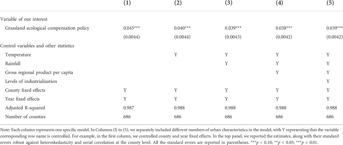
TABLE 1. Estimates in the impact on grassland quality from difference-in-differences estimators.

The first column of this table does not control for any county characteristic. In a pattern similar to all of the estimates that we presented, we found a statistically significant amount of average impact on grassland quality, with a coefficient on the GECP of 0.045.

Column 2, controlling for temperature, shows that the estimate in the impact of the GECP on grassland quality is similar to that found in Column 1.

Column 3 adds temperature and rainfall, showing that average change in grassland quality around the introduction of the GECP is analogous to that of Column 2.

Column 4 includes three control variables: temperature, rainfall, and gross regional product per capita. The estimated coefficient on our variable of the GECP here remains similar to those reported in the previous columns.

Columns 5 absorbs four controls of county characteristics. We found that the results, obtained from the last column, was very close to those in the first four columns. The coefficient of the variable of our interest is now 0.039, indicating that the GECP increased annual grassland quality by about four percentage points.

Overall, these results boost our confidence: they are not driven by chance and are extremely robust by including different numbers of county characteristics. Motivated by this, we pay attention to the specification in Column 5, controlling for a rich collection of county characteristics, as well as fixed effects, for the results from the event study, further robustness check, and heterogeneity analysis. We refer to these estimates here as baseline results.

3.1.2 Propensity-score-matching difference-in-differences estimates

Table 2 reports the estimates obtained from our propensity-score-matching difference-in-differences estimator, adjusted for different numbers of county characteristics. In Table 2, we present the estimates of the impact of the GECP on grassland quality, along with their standard errors which are robust against heteroskedasticity and serial correlation at the county level. To compare the results in Table 2 with those in Table 1, we used the controls in one column of Table 2 just as we did in the corresponding column of Table 1. That is, each column of Tables 1 and 2 have the same specification. In line with our expectation, the estimates from our propensity-score-matching difference-in-differences estimators are very similar to those from the baseline models, although there is a small difference between them, with an estimated coefficient of the GECP ranging from 0.045 to 0.058.

TABLE 2. Estimates in the impact on grassland quality from propensity-score-matching difference-in-differences estimators.

3.1.3 Inverse-probability-weighting difference-in-differences estimates

Table 3 presents the results obtained from the inverse-probability-weighting difference-in-differences estimator, adjusted for different numbers of county characteristics. In Table 3, we present the estimates of the impact of the GECP on grassland quality, along with their standard errors robust against heteroskedasticity, and serial correlation at the county level. To allow these results reported here to be compared with baseline results, as well as with those in Table 2, we adopted in Columns 1 to 5 of Table 3 the specifications from the same six columns of Table 1. We found that the results were similar across the three tables, with a substantial increase in county employment—indicating that the estimated results are extremely robust to the choice of econometric models. Of course, the results suggest that the control group is comparable to the treated group before introducing the GECP into the raw sample.

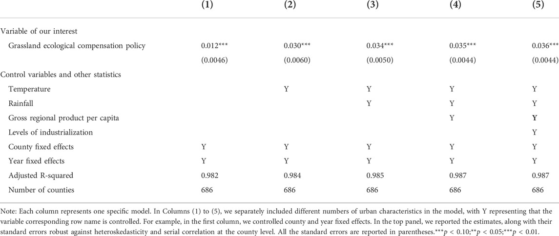
TABLE 3. Estimates in the impact on grassland quality from inverse-probability-weighting difference-in-differences estimators.

3.2 Tests for parallel trends assumption

We conducted event studies to investigate the evolution of the trends in grassland quality in the treated and control groups. This analysis allows us to check whether their trends are similar to before the introduction of the GECP. We also investigated the dynamics of grassland quality after the introduction of the GECP, helping us to check whether the policy has an instantaneous impact on grassland quality, as well as whether its effect on grassland quality is persistent.

Figure 1 plots our findings. It is structured in three panels. In the top panel, we depicted the estimates of the dynamic impacts of the GECP on grassland quality from our preferred specification by fitting a difference-in-differences estimator, along with their 95% confidence intervals constructed using standard errors robust against heteroskedasticity, and serial correlation at the county level. In the middle panel, we depicted the estimates of the dynamic impacts of the GECP on grassland quality from our preferred specification by fitting a propensity-score-matching difference-in-differences estimator, along with their 95% confidence intervals constructed using standard errors robust against heteroskedasticity and serial correlation at the county level. In the bottom panel, we depicted the estimates of the dynamic impacts of the GECP on grassland quality from our preferred specification by fitting an inverse-probability-weighting difference-in-differences estimator, along with their 95% confidence intervals constructed using standard errors robust against heteroskedasticity and serial correlation at the county level. In each panel, the blue points represent the estimates of the dynamic impacts of the GECP on grassland quality, while the blue lines represent their 95% confidence intervals, with the values of years equal to 0 corresponding to the year of launch of the GECP.

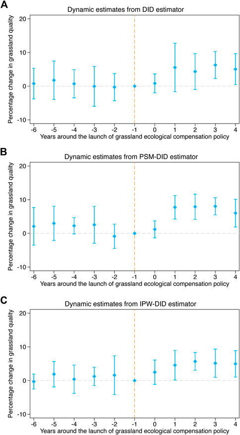
FIGURE 1. Dynamic estimates.

Across the three figures, we found a similar pattern in the dynamics of grassland quality. That is, before the introduction of the GECP, although the difference in trends of grassland quality between the treated group and the control group exhibit a slightly upward trend, all the coefficients are statistically insignificant, implying that the parallel trends assumption could be reasonable if the GECP had not been launched. However, we observe that, after introducing the GECP, grassland quality in the treated group clearly increases during subsequent periods, indicating that the GECP might have an immediately positive impact on grassland quality with a persistent increase in grassland quality.

3.3 Further robustness check

In Figure 2, we further investigate the robustness of our estimates of the impact of the GECP on grassland quality by implementing a series of statistical tests. In Figure 2A, we performed the leave-one-county-out test. The red line represents the raw estimate from our preferred specification, which is reported in Column 5 of Table 1. Using the same specification, we obtained 686 estimates of the impact from the 686 leave-one-county-out samples. The blue lines represent the 95% confidence intervals of these estimates, which are constructed using their standard errors robust to heteroskedasticity and serial correlation at the county level. We found that all the 95% confidence intervals contain the raw estimate represented by the red line, suggesting that our results are robust to selection of an individual unit.

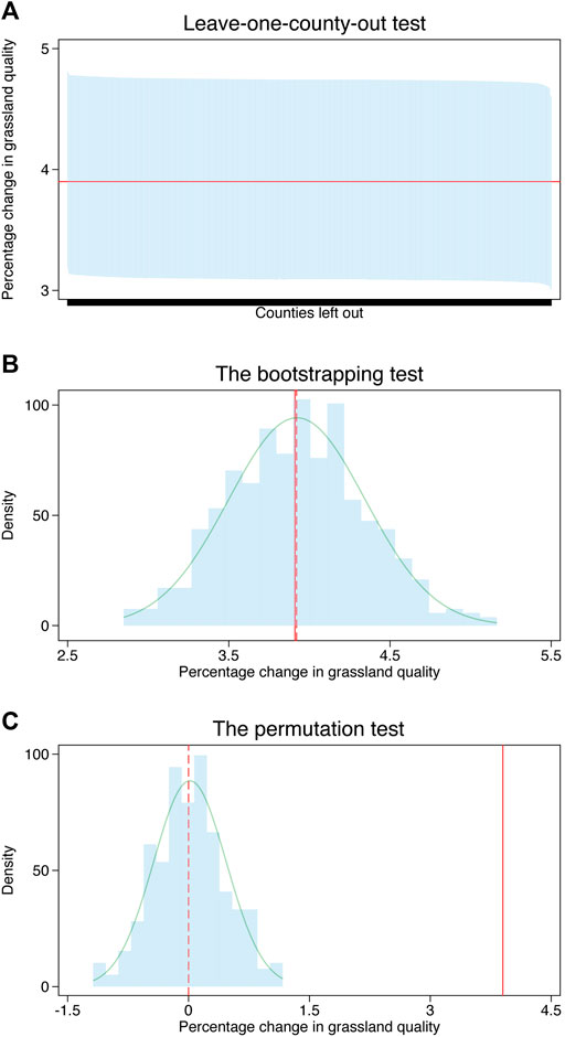
FIGURE 2. Robustness check.

In Figure 2C, we performed the bootstrapping test with 1,000 random samples. The red solid line represents the raw estimate from our preferred specification reported in Column 5 of Table 1, while the red dash line represents the mean of the empirical distribution of these estimates from the bootstrapping test. The blue shadow is the empirical distribution and the green curve is the fitted normally distributed curve for the empirical distribution. We found that the mean of the empirical distribution is similar to the raw estimate and is also far from zero, implying that our results are not sensitive to sample selection.

In Figure 2C, we performed the permutation test with 1,000 random samples, randomly assigning a treatment or control to counties. The red solid line represents the raw estimate from our preferred specification reported in Column 5 of Table 1, while the red dashed line represents the mean of the empirical distribution of these estimates from the permutation test. The blue shadow is the empirical distribution and the green curve is the fitted normally distributed curve for the empirical distribution. We found that the mean of the empirical distribution approaches zero but is far from the raw estimate, indicating that our results are again robust, and economically and statistically significant.

3.4 Heterogeneity analysis

In Figure 3, we investigated whether the impact of the GECP on grassland quality varied across different county characteristics. Note that the analysis of heterogeneous impacts does not have a causal interpretation; however, it is beneficial to understand the potential channels through which the GECP had an impact on grassland quality.

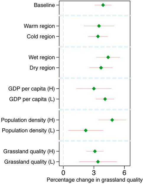
FIGURE 3. Heterogeneity analysis.

Firstly, we investigated whether the impact on grassland quality of the GECP would be dependent on temperature and rainfall. We observed that the impact was similar whether counties were located in warm or cold regions. We also found that the GECP had a larger impact on grassland quality in wet than in dry regions.

In the middle section of Figure 3, we examine the impact heterogeneity corresponding to economic development status and county population size. We found that the impact of the GECP on grassland quality might be dependent on levels of economic development and population density. That is, in richer and more population counties, the GECP had a larger impact on grassland quality.

Finally, the bottom section of Figure 3 shows that the impact of the GECP on grassland quality in counties with a higher level of grassland quality was larger than that in counties with a lower level of grassland quality.

In short, the results from heterogeneity analysis suggest that the impact of the GECP on grassland quality is not evenly distributed across different types of county.

4 Conclusion

In this article, we provided evidence that payment for ecological services programs had a significant and robust positive impact on grassland quality by focusing on China’s GECP, which is the planet’s largest. This result remains true with difference-in-differences estimators that compare counties which have and have not introduced the low-carbon pilot project while controlling for county characteristics, as well as propensity-score-matching difference-in-differences that estimates the propensity a county launching the GECP. Our preferred specifications show that the average reduction in grassland quality is about four percentage points around the introduction of grassland ecological compensation policy.

We also used the propensity score as a weight to balance county characteristics between the treated group and the control group. Using the inverse-probability-weighting difference-in-differences estimator, we again confirmed that the GECP had a positive impact on grassland quality.

The triangulation of evidence, from the three difference-in-differences estimators, all leads to a similar estimate in the impact of the GECP on grassland quality, giving us confidence that there is a positive causal effect of the GECP on grassland quality. Our results also show that the GECP has a greater impact on grassland quality in warmer, richer, and higher grassland quality-level counties than in those with opposite characteristics.

In sum, our results suggest that there is a persistent increase in grassland quality around the introduction of the GECP. Work using a fully comprehensive dataset to investigate the potential mechanisms through which the GECP affects grassland quality is an obvious and fruitful area for future research. Another important field of future inquiry is an exploration of whether the impact of the GECP on grassland quality is dependent on the ability of government to manage the economy, as well as the degree to which a county is being converted from a planned economy to a market economy.

Data availability statement

Data are available from the corresponding author upon reasonable request.

Author contributions

All authors equally contributed to this paper. CW conceptualized the study and provided supervision. JK collected data, conducted the statistical analysis, and drafted the manuscript. YZ conducted the statistical analysis and completed the revision. CW, YZ, and JK contributed to the interpretation of the results. All authors provided critical feedback on drafts and approved the final manuscript.

Funding

We acknowledge funding from the National Social Science Foundation of China (Grant no. 18ZDA051), the National Natural Science Foundation of China (Grant no. 72171100), the National Natural Science Foundation of China (Grant no. 72073049), the National Natural Science Foundation of China (Grant no. 71703052), the Natural Science Foundation of Hubei Province (Grant no. 2020CFB853), and the Science and Technology Project of State Grid Corporation of China (Grant no. B311JH21000D and B311UZ21000D). This paper does not reflect an official statement or opinion from the organizations.

Acknowledgments

We thank Botao Liu, Yu Cao, Lang Cheng, Wei Wei, and Yihui Li for their helpful comments on an earlier version of this article. In addition, JK wants to particularly thank the patience, care, and support of Ying Nie over the years.

Conflict of interest

The authors declare that the research was conducted in the absence of any commercial or financial relationships that could be construed as a potential conflict of interest.

Publisher’s note

All claims expressed in this article are solely those of the authors and do not necessarily represent those of their affiliated organizations, or those of the publisher, the editors and the reviewers. Any product that may be evaluated in this article, or claim that may be made by its manufacturer, is not guaranteed or endorsed by the publisher.

References

Baker, A. C., Larcker, D. F., and Wang, C. C. Y. (2022). How much should we trust staggered difference-in-differences estimates? J. Financial Econ. 144, 370–395. doi:10.1016/j.jfineco.2022.01.004
Bertrand, M., Duflo, E., and Mullainathan, S. (2004). How much should we trust differences-in-differences estimates. Q. J. Econ. 119, 249–275. doi:10.1162/003355304772839588
Börner, J., Baylis, K., Corbera, E., Ezzine-de-Blas, D., Honey-Roses, J., Persson, U. M., et al. (2017). The effectiveness of payments for environmental services. World Dev. 96, 359–374. doi:10.1016/j.worlddev.2017.03.020
Cao, S., Chen, L., and Yu, X. (2009). Impact of China's grain for green project on the landscape of vulnerable arid and semi-arid agricultural regions: A case study in northern shaanxi Province. J. Appl. Ecol. 46, 536–543. doi:10.1111/j.1365-2664.2008.01605.x
Chen, Y., Wang, K., Lin, Y., Shi, W., Song, Y., and He, X. (2015). Balancing green and grain trade. Nat. Geosci. 8, 739–741. doi:10.1038/ngeo2544
Deng, L., Shangguan, Z.-p., and Li, R. (2012). Effects of the grain-for-green program on soil erosion in China. Int. J. Sediment Res. 27, 120–127. doi:10.1016/s1001-6279(12)60021-3
Ding, Z., and Yao, S. (2021). Ecological effectiveness of payment for ecosystem services to identify incentive priority areas: Sloping land conversion program in China. Land Use Policy 104, 105350. doi:10.1016/j.landusepol.2021.105350
Freyaldenhoven, S., Hansen, C., and Shapiro, J. M. (2019). Pre-event trends in the panel event-study design. Am. Econ. Rev. 109, 3307–3338. doi:10.1257/aer.20180609
Hayes, T., Murtinho, F., Wolff, H., López-Sandoval, M. F., and Salazar, J. (2022). Effectiveness of payment for ecosystem services after loss and uncertainty of compensation. Nat. Sustain. 5, 81–88. doi:10.1038/s41893-021-00804-5
Hou, L., Xia, F., Chen, Q., Huang, J., He, Y., Rose, N., et al. (2021). Grassland ecological compensation policy in China improves grassland quality and increases herders’ income. Nat. Commun. 12, 4683. doi:10.1038/s41467-021-24942-8
Hu, Y., Huang, J., and Hou, L. (2019). Impacts of the grassland ecological compensation policy on household livestock production in China: An empirical study in inner Mongolia. Ecol. Econ. 161, 248–256. doi:10.1016/j.ecolecon.2019.03.014
Imai, K., Kim, I. S., and Wang, E. H. (2021). Matching methods for causal inference with time-series cross-sectional data. Am. J. Political Sci. doi:10.1111/ajps.12685
Kleijn, D., and Sutherland, W. J. (2003). How effective are European agri-environment schemes in conserving and promoting biodiversity? J. Appl. Ecol. 40, 947–969. doi:10.1111/j.1365-2664.2003.00868.x
Liu, M., Dries, L., Heijman, W., Huang, J., Zhu, X., Hu, Y., et al. (2018). The impact of ecological construction programs on grassland conservation in inner Mongolia, China. Land Degrad. Dev. 29, 326–336. doi:10.1002/ldr.2692
Morrish, N., Mujica-Mota, R., and Medina-Lara, A. (2022). Understanding the effect of loneliness on unemployment: Propensity score matching. BMC public health 22, 740. doi:10.1186/s12889-022-13107-x
Sant’Anna, P. H. C., and Zhao, J. (2020). Doubly robust difference-in-differences estimators. J. Econ. 219, 101–122. doi:10.1016/j.jeconom.2020.06.003
Sims, K. R. E., and Alix-Garcia, J. M. (2017). Parks versus PES: Evaluating direct and incentive-based land conservation in Mexico. J. Environ. Econ. Manag. 86, 8–28. doi:10.1016/j.jeem.2016.11.010
Whittingham, M. J. (2011). The future of agri-environment schemes: Biodiversity gains and ecosystem service delivery? J. Appl. Ecol. 48, 509–513. doi:10.1111/j.1365-2664.2011.01987.x
Wu, J., and Lin, H. (2010). The effect of the conservation reserve program on land values. Land Econ. 86, 1–21. doi:10.3368/le.86.1.1
Zhai, G., Xie, K., Yang, D., and Yang, H. (2022). Assessing the safety effectiveness of citywide speed limit reduction: A causal inference approach integrating propensity score matching and spatial difference-in-differences. Transp. Res. Part A Policy Pract. 157, 94–106. doi:10.1016/j.tra.2022.01.004
Keywords: grassland ecological compensation policy, grassland quality, program evaluation, difference-in-differences, matching
Citation: Wei C, Zhou Y and Kong J (2022) Evidence regarding the ecological benefits of payment for ecological services programs from China’s grassland ecological compensation policy. Front. Environ. Sci. 10:989897. doi: 10.3389/fenvs.2022.989897
Received: 09 July 2022; Accepted: 25 August 2022;
Published: 30 September 2022.
Edited by:
Salvador García-Ayllón Veintimilla, Technical University of Cartagena, SpainCopyright © 2022 Wei, Zhou and Kong. This is an open-access article distributed under the terms of the Creative Commons Attribution License (CC BY). The use, distribution or reproduction in other forums is permitted, provided the original author(s) and the copyright owner(s) are credited and that the original publication in this journal is cited, in accordance with accepted academic practice. No use, distribution or reproduction is permitted which does not comply with these terms.
*Correspondence: Jiayang Kong, jiayangkong@hotmail.com
†These authors have contributed equally to this work