Mediating Sustainability and Liveability—Turning Points of Green Space Supply in European Cities

Introduction

The draft action plan of the Urban Agenda for the EU acknowledges that Europe is one of the most urbanized areas of the world with more than 70% of Europe's citizens being urbanites, and with an expected increase to 80% by 2050 (Netherlands Presidency, 2016). Artificial areas, with the exception of urban green and sport/leisure areas, are expected to increase from 3.6 to 4.3% of the entire land surface [own calculation based on 2000 to 2018 trend following EEA (2017), Copernicus (2019)]. This 0.7%-point increase until 2050 corresponds to an area almost the size of the Netherlands and is commonly related to urbanization. This also raises economic, social and environmental challenges as land is a scarce resource (McPhearson et al., 2016; Elmqvist et al., 2017).

In order to make cities more environmentally sustainable and improve liveability, the European Commission promotes the Compact City Model (Commission of European Communities, 1990). In this model, which is widely used among scholars and planners, density is seen as a critical characteristic in determining sustainable and liveable urban forms (Burton, 2000; Duany et al., 2001; Hall, 2001). However, the degree of density, defined as the ratio of people, jobs or dwellings to a specified reference area, indicates a dilemma between high and low densities (Wiersinga, 1997). Residential density is, for instance, the ratio of residents per residential area. “For a city to be sustainable, the argument goes, functions and population must be concentrated at higher densities. Yet for a city to be liveable, functions and population must be dispersed at lower densities” (Neumann, 2005, p. 16, see Figure 1).

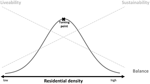
Figure 1. Balance between sustainability and liveability depending on residential density.

Scholars underline that high residential densities in cities mean shorter journeys to work and services, more walking, cycling or use of public transport, better access to green spaces and other facilities, or encouraged social interaction (Jabareen, 2006; Masnavi, 2007). Lower fuel emissions, less ground space per capita and reduced energy costs due to apartments in multi-family houses or blocks that require less heating are added environmental benefits that conserve resources and are seen as tackling the problem of unsustainability (Jabareen, 2006; Westerink et al., 2013). Cities need a certain residential density for infrastructure networks and facilities such as roads, drainage and sewerage, electricity, telecommunication run more efficiently and economically (Westerink et al., 2013). However, if residential density exceeds a certain limit, these systems can be overloaded (Cheng, 2009).

Many cities struggle with social, economic, and environmental problems resulting from high densities. The increasing concentration of people, activities and facilities is associated with the overuse of infrastructure, social inequity due to the higher cost of land, privatization of some urban spaces, traffic congestion, and air pollution (Weber et al., 2014; Haase, 2016). In particular, land sealing and the extension of the urban fabric onto open land or brownfields increasingly puts green and open space in cities under pressure (Haase, 2008; Herrmann et al., 2016). Consequently, low densities offer multiple benefits such as fresh air, oxygen supply, tree shade, habitats for species, and also make cities more liveable (Neumann, 2005; Kabisch and Haase, 2013).

Cities seek to find a compromise between high and low densities because the number of people within a given area “becomes sufficient to generate the interactions needed to make urban functions viable” (Jabareen, 2006, p. 41). This is related to the concept of turning points, which indicate an optimal compromise between high and low densities (Figure 1). In this paper we will apply the concept of turning points to the relation between residential density and green space supply, following up on previous research which just studied green space supply but not potential demand by urban dwellers (Fuller and Gaston, 2009; Kabisch and Haase, 2013).

Green spaces in cities contribute to the mitigation of and adaptation to climate change, minimize the risks of natural disaster, and support biodiversity conservation by cooling, noise reduction and air filtration of pollutants (Kabisch et al., 2015). They are places of recreation, encounter or sport, improve the quality of the neighborhood, and promote physically active lifestyles and healthy behavior (Reyer et al., 2014; Wüstemann et al., 2017). Different types of green space have different qualities and functions. While public urban parks play a major role as recreational spaces, all vegetated areas are crucial as habitats for urban flora and fauna or physical functions such as carbon sequestration and storage (Kowarik, 2011; Beninde et al., 2015).

The higher the green space provision in a city, the higher are the potential ecological functions of the green spaces. Residential density indicates the demand for green spaces—the lower it is, the lower is the corresponding pressure on green spaces. In contrast, the higher the residential density, the more people benefit from green space functions. Consequently, cities have to balance the natural environment with human development—the sustainable and the liveable city (Neumann, 2005; Pauleit et al., 2005). Certainly, a constant equilibrium in cities is not realistic as they are open and dynamic systems that are “subject to human will and caprice as well as the furies and salves of nature” (Neumann, 2005, p. 19). However, the balance concept is useful in order to measure to what extent the green space provision in cities does meet the green user demand following the ecology of cities concept (Grimm et al., 2008; Herrmann et al., 2016; Reyers and Selomane, 2018). Green spaces do not just supply population but also experience pressure at a certain demand level. If residential densities exceed a certain limit, overuse and overcrowding of green spaces can lead to a decline in the provision of ecosystem services (Burkhard et al., 2012 Villamagna et al., 2013).

Despite all the success stories about greening cities (Rouse and Bunster-Ossa, 2013; Mell, 2015; Hansen et al., 2016), the question as to what extent cities balance the population demand for recreation with the provision of green spaces remains unanswered. In their analysis of urban green spaces in more than 300 European cities for the year 2000, Fuller and Gaston (2009) suggested that density and green space share are uncoupled. In contrast, Kabisch and Haase (2013), in their analysis of urban green spaces in 202 European cities for 2006, found a significant positive relation between higher green space share and an increased density in cities. While Kabisch and Haase (2013) found that population density and per capita green space supply is not correlated, Fuller and Gaston (2009) saw a drop in per capita green with increasing density. These findings are not contradictory as different density concepts have been used. Kabisch and Haase (2013) related density to total area (within the administrative boundaries, gross density) while Fuller and Gaston (2009) related density to built-up area (net density). Both studies detect differences between European regions and concluded that the green space share is not associated with population size of a city. Similar, in his analysis of forest areas and urban green spaces for 2012 in almost 400 cities, (Poelman, 2016) concluded that the overall population size of a city is uncoupled from the green space supply.

Although these studies effectively report and discuss the provision of green spaces in European cities, they lack a systematic answer to the question of to what extent the provision of green spaces meets the potential population demand, and to what extent differences between types of green can be detected. Against this background, we will develop an understanding of green space supply and its relation to the residential density of cities. Therefore, we conceptualize green space supply as an indicator that measures how green space provision and residential densities are related. Variations in the green space supply indicate how low and high densities are mediated and where potential turning points are. The analysis of 905 European is conducted around the following three questions:

1. How are cities of different residential densities performing in terms of green space supply?

2. What are turning points in the relation between green supply and residential density?

3. How do cities balance green space supply and green space pressure in Europe?

Materials and Methods

Our analysis is based on a sample of 905 European cities that are covered in the Urban Atlas database (Copernicus, 2018). The Urban Atlas provides reliable, comparable, high-resolution land use and land cover data for the 2012 reference year in 36 EEA member and cooperating countries. Cities represent local administrative units with a population of at least 50,000 inhabitants (11 cities were smaller in 2012). The nomenclature includes 17 urban classes with a minimum mapping unit (MMU) of 0.25 ha and 10 rural classes with a MMU of 1 ha. Figure 2 shows that we only considered land uses within the administrative core cities which have been defined using the Urban Audit delineation and OSM boundaries for the Western Balkans (EG, 2018; OSM, 2019). In order to contrast the results with the aforementioned previous studies (Fuller and Gaston, 2009; Kabisch et al., 2016) and to make the results more robust, we calculated two green space types: urban green spaces are defined using class 141 (green urban areas which basically cover parks, public gardens or cemeteries, Figure 2), whereas total green space was defined by the classes 141 and 310 (forest). In keeping with other studies, we only considered green spaces within 300 meters of residential areas that have been calculated by creating buffers around residential areas (Handley et al., 2003; Kabisch et al., 2016; Poelman, 2016; Wüstemann et al., 2017).

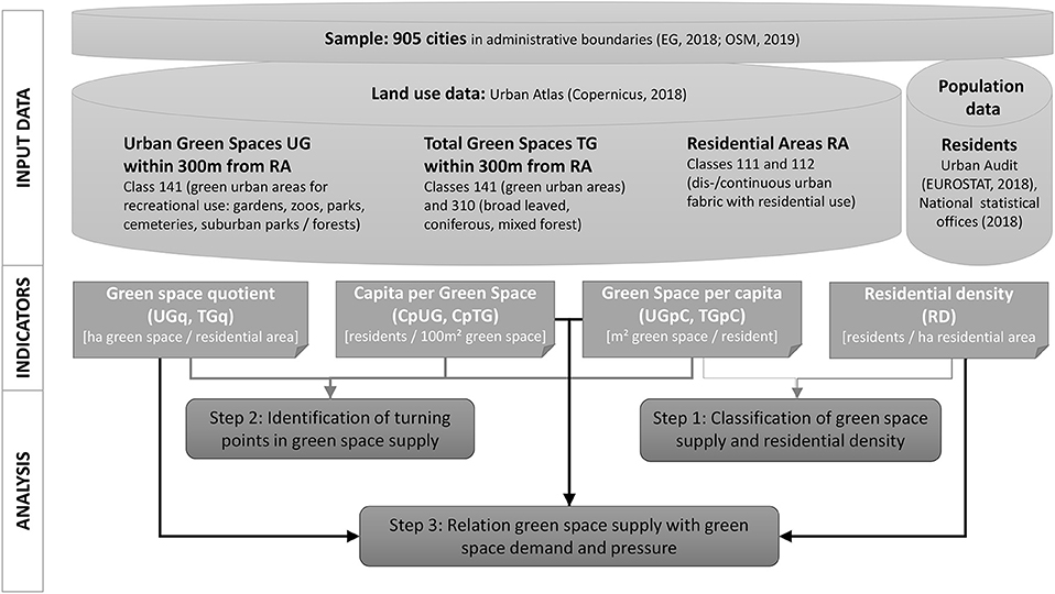
Figure 2. Workflow of the study.

The following four indicators have been calculated:

In order to estimate the green space demand of a city, we calculated Residential Density (RD), defined as the ratio between residents and their residential area. Using RD allows conclusions to be drawn about the built-up structure (Frey, 1999; Masnavi, 2000; Kasanko et al., 2006; Westerink et al., 2013) and for green space demand (Fuller and Gaston, 2009). The 2012 population numbers have been obtained from the Urban Audit database (EUROSTAT, 2018). In the case of gaps, data from national statistics have been used and carefully counterchecked for comparability and correctness.

The green space provision, usually calculated as the green space share of total area, is related to the residential area, as this indicator is not sensitive to the total area of a city (Fuller and Gaston, 2009) and corresponds with the other indicators used (Figure 2). Consequently, we defined the Green Space Quotient as the area in ha which is available for one ha residential area (UGq for urban green spaces, TGq for total green spaces). The Green Space per capita UGpC and TGpC is expressing the supply of green spaces per resident. Additionally, we calculated the Capita per Green Space as the number of residents per 100 m² green spaces (CpUG, CpTG) in order to mirror the population pressure on green spaces.

The analysis involves three steps that structure the results (Figure 2).

In a first step, we developed a descriptive typology in which we contrast classes of green supply and residential density. We classify green space supply into below average supply (<9 for UG, <45 m²/capita for TG), average supply (9 to <18 for UG, 45 to <90 m²/capita for TG) and above average supply (≥18 for UG, ≥90 m²/capita for TG) referring to the WHO criteria of 9 m² green/person within 300 meters (WHO, 2012). For residential densities, we created three classes according to quantiles of the sample group in order to avoid a normative target value: low density, dense and high residential density (<65, 65 to <90, ≥90 residents/ha). We analyzed difference in geographic location using the ESPON WUTS 4 regional classification (ESPON, 2014) and ANOVA analysis.

In a second step, we systematically conceptualized the relation between RD, green space supply (UGpC, TGpC), green space provision (UGq, TGq) and green space pressure (CpUG, CpTG) using correlation analysis (Spearman's rho) and trend curve calculations with LOESS algorithm (Locally weighted scatterplot smoothing with 3 polynomial of degree for cities with a RD of ≤200 residents/ha in order to exclude outliers; Cleveland, 1981). LOESS was chosen as it provides the lowest residues compared to other curve fitting algorithms while it has the potential to detect potential turning points, since LOESS does not assume linear relations (Talgorn et al., 2018). We detect turning points which are defined as residential density for which the green space supply is maximized in line with Figure 1.

A third step calculates the ratio between green supply and green pressure (UGpC/CpUG). A ratio of 1 indicates that CpUG = UGpC = 10 m²/resident. This value was derived from the WHO criteria of providing a minimum of 9 m²/resident. However, this value was rounded in order to simplify the formula symbol for the green space pressure which was defined as residents/100 m². Consequently, a ratio of 1 was defined as the cutting point which indicates that the pressure on green spaces is so high that the supply becomes insufficient. Ratios below 1 indicate a green space pressure exceeding the green space supply. The higher the ratio, the higher the green space supply (UGpC) and the lower is the green space pressure (CpUG). Based on the ratio, we derived seven classes by applying identical thresholds based on quantiles as class breaks. We plotted the seven classes in a graph for which we use (UGpC) as a central indicator for measuring how much green spaces (UGq) cities provide under different RD in order to archive a certain green space supply (UGpC). Finally, we contrasted our results with the performance of Europe's green capitals as they have been awarded not just by quantitative values but also because of successful greening measures (EC, 2019).

Results

Differences in Green Space Supply in European Cities

The average green space supply for UG (UGpC) in European cities in 2012 was 14 m²/resident (numeric median). However, there are significant regional differences (Figure 3). Whereas, Northern European cities show comparably high UGpC values (median 21 m²/resident), cities in Southern Europe and the Balkan show significantly lower values with a median of 6 m²/resident. The median UGpC values of Western and Eastern European cities range above the European average with 17 and 15 m²/resident, respectively. The majority of cities in Northern Europe show an above average supply, in Western Europe, an above or average supply, in Eastern Europe, an average supply and, in Southern Europe as well as the Balkans, an below average supply (Table S1). Considering the TGpC, the difference between Northern and Southern Europe disappears because Western and Eastern European cites report the highest median values with 58 m²/resident each. The median of 43 m²/resident in Northern Europe is close to the European average (44 m²/resident) while cities in Southern Europe and the Balkans again show low values of 19 and 18 m²/resident. There are basically two reasons for differences between the supply of the two green types.

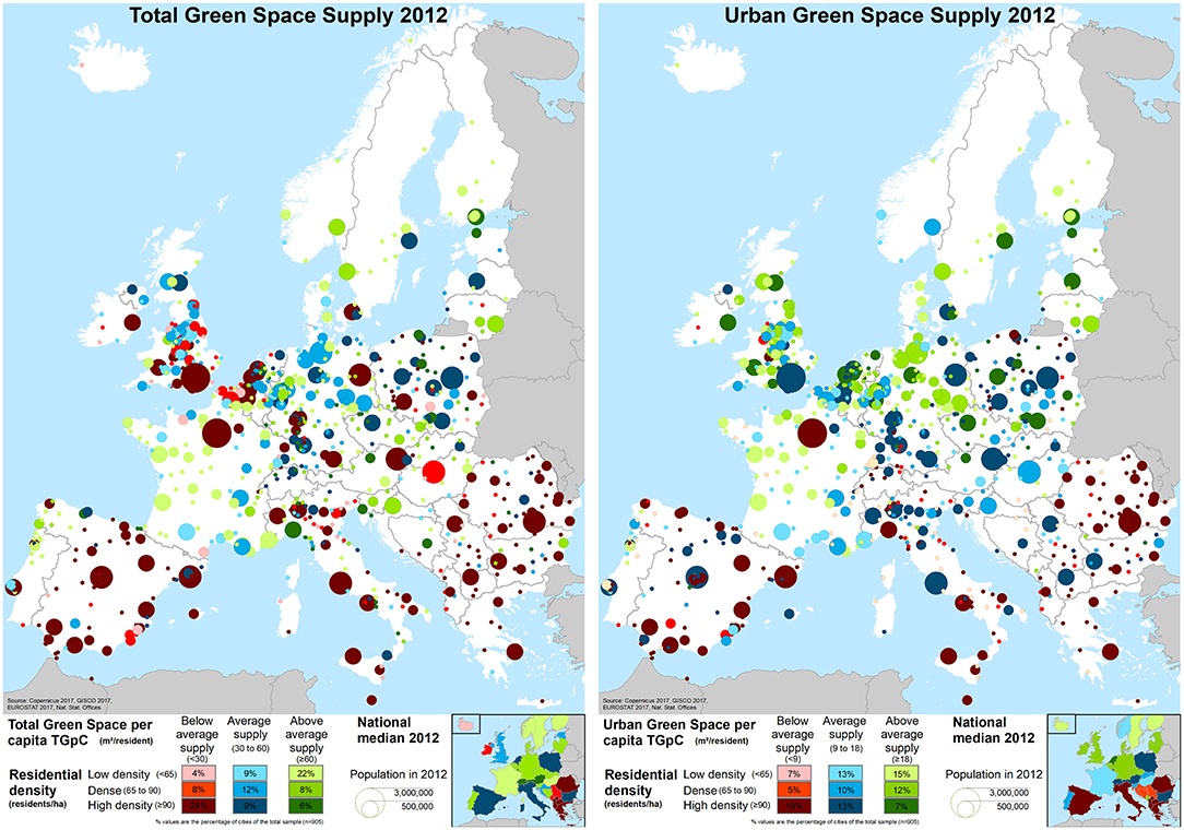
Figure 3. Typology of green space supply in different residential density classes.

First, intra-regional variations can be observed in almost all regions. While cities in the British Isles lack forested areas, Scandinavian cities usually contain high shares of forest areas, such as in Oslo (Figure 3). Moreover, cities in Eastern and even Southern Europe have a comparably higher share of forest areas (Figure S1). Second, city size plays a very important role for the green supply. While larger cities report a lower TGpC class then for UGpC, such as in the Randstad, cities in the Po valley, as well as several capitals all over the continent, smaller cities are basically in a higher TGpC class then for UGpC (Figure 3). Examples in France, Germany, Poland, Romania, Italy, and Spain benefit from forest areas. A weak but significant correlation (0.239, Table S2) suggests that the larger a city in population size, the higher the share of UG on TG. An even higher correlation (0.447) can suggest for residential density that the denser a city in Europe is, the higher is its dependency on urban green while smaller cities tend to benefit more from other green space types.

Figure 3 contrasts three classes of residential density (low dense, dense, high dense) with the green supply classes of UGpC and TGpC (below average, average, above average). The majority of cities perform as expected from the preceding analysis for both green types UG and TG. For UG high residential density cities usually show below average supply (18%, the percentage value refers to the type of the total sample of cities as displayed in Figure 3). In particular, in Southern Europe and the Balkans, dense cities have average supply (10%). Low residential density cities have an above average supply (15%) in particular in Western and Northern Europe (Table S1). For TG, even more cities follow this tendency (24%, 12%, 22%). In particular, the below average supply of TG in high residential density areas is not limited to Southern Europe but characterizes many large cities all over the continent. This underlines the relationship between city size and the importance of UG mentioned above.

However, several cities show a higher green space supply than the average constellation between residential density and green space supply described above suggests. High density cities in Germany, Poland or capitals in Southern Europe and the Balkans have an average supply for UG (13%) while average density cities, such as in Eastern Germany or the UK, show an above average supply. Even some high density cities show an above average supply of UG (7%), such as in the British Isles, in some capitals of Scandinavia and the Baltics, or Eastern Europe. For TG, high density cities hardly show an above average supply except for a few small cities in Italy, the Czech Republic, and Poland.

Finally, cities on the French Mediterranean coast, in Norway, and Eastern Europe only have an average supply, even though their residential density is low (13%). This is even more characteristic in dense (e.g., Cordoba, Wrexham) or even low density cities such as Mulhouse, which show a below average supply for UG. For TG, such an below average supply can also be found in dense cities such as in Spain, in the Midlands, Bucarest, or Lille as well as in low density cities such as Caen, Gent, Elche or Czestochowa.

Turning Points in the Relation Between Green Supply and Residential Density

The classification of residential densities allows to explore the relationship between green space supply and residential density. A corresponding correlation coefficient confirms this significant relation which is, however, stronger for TG then for UG (-0.365 for UGpC and −0.643 for TGpC, Table S2). This is due to the different relation between green space provision and residential density. The two corresponding correlation coefficients suggest that the denser a city is, the lower is its green space provision of TG (−0.219 for TGq) but the larger is its green space provision of UG (0.312 for UGq).

For UG, this means, firstly, that the drop in total green space supply with increasing residential density is compensated by high green space provision of UG. This is shown in Figure 4 (top), in which an increasing residential density (RD) is contrasted with a linear increasing green space provision (UGq, the regression coefficient is used as slope). The resulting green space supply for UG (UGpC) drops at a slower rate than the supply for TG (TGpC).

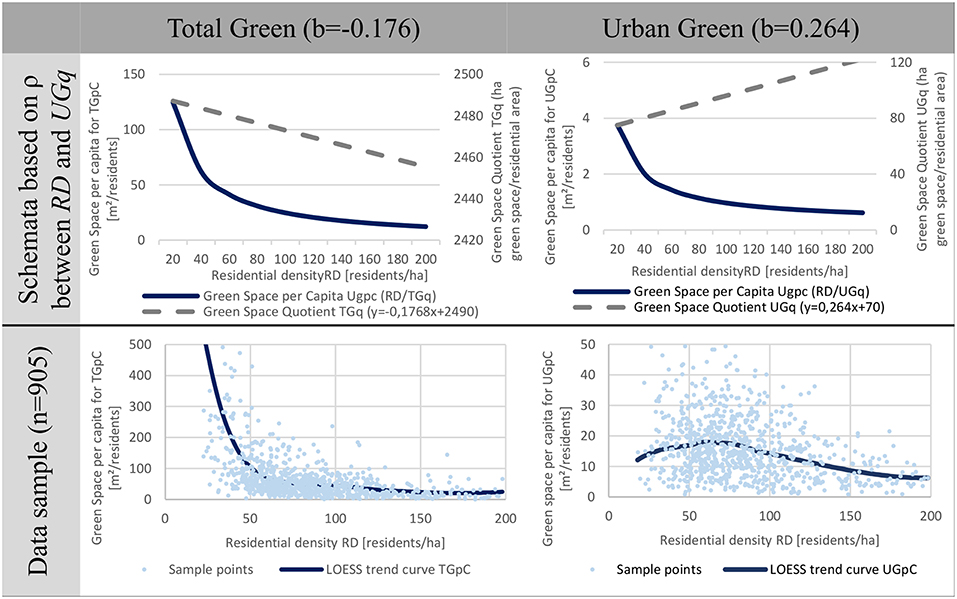
Figure 4. Schematic trend curve of green space supply based on correlation coefficient (top,) compared to the LOESS trend curve of the actually measured green space supply (down).

Secondly, it shows that the two green space types have a different relationship to residential density. Comparing the LOESS trend curve for the data sample with the schematic curve based on the correlation coefficient shows that both curves are similar for TG (Figure 4 left). In contrast, the curves differ for UG (Figure 4 right) as the LOESS trend curve increases among low densities and decreases among high densities along the gradient of residential density. The different relation is also mirrored by the correlation between residential density and green space supply for the residential density classes used in the first result section. At the same time, for TG, the relation is significantly negative throughout all residential density classes and a significant negative relation for UG can only be measured for high density cities (>90 residents/ha).

Consequently, we will focus on UG in the next section and contrast the LOESS trend curves of green supply (UGpC), green pressure (CpUG), and green provision (UGq) against the gradient of residential densities within our sample of cities displayed in Figure 5.

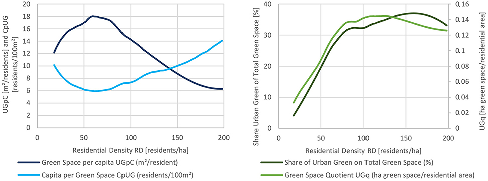
Figure 5. LOESS trend curves for green space supply (UGpC), pressure (CpUG), provision (UGq), and share of Urban Green on Total Green Space plotted against residential density (RD) for a sample of 905 cities.

UGpC is low on average in low density cities as a result of the low UGq values. However, this low green space supply is compensated by TG, e.g., by forest areas as the share of UG on TG is very low (Figure 5). With increasing residential densities, the UGpC value increases, as a consequence of an increased green space provision (UGq). In consequence, the green space pressure (CpUG) decreases. However, the green space supply does not increase limitlessly with increasing residential density. At a certain point, UGpC reaches a maximum and CpUG bottoms out—a turning point. This is due, first of all, to an increasing green space demand in terms of a higher residential density, and secondly, to the fact that green space provision becomes saturated at a high level. With increasing residential density, the green space pressure increases but can hardly be compensated for by other green types such as forests. UG is already very important for the green supply in these cities and exceeds 30% share on TG.

With further increase in residential density the green space pressure (CpUG) exceeds the green space supply (UGpC) as a consequence of the increasing population demand and a decreasing green space provision (UGq)—a cutting point. In high density cities, the share of UG on the total area decreases which is not fully compensated by the increasing share of other green spaces such as forests.

There is a large variation in the green space supply among European cities. However, the UGpC values of 77% of all cities range between ± 1SD around the LOESS trend curve for UGpC. This close fit between the actual and the predicted values is particularly visible in Western and Eastern European cities. A higher positive deviation (> +1SD) indicates that a higher curve maximum can be recorded for Northern European cities while, for cities in the Balkans and especially Southern Europe, the deviation is below − 1SD (Figure S2). Due to lower shares of UG, the number of cities with deviations below − 1SD is particularly large among small cities.

From the relations between the left trend curves in Figure 5, two inflection points can be derived, which we demonstrate by calculating the ratio between both indicators (UGpc/CpUG): the cutting point in which the green space pressure CpUG exceeds the green space supply UGpC indicated by a ratio below 1, and the turning point in which UGpC is maximized and CpUG is lowest. The larger the ratio, the more balanced is the city green supply and pressure, and the higher is the resulting UGpC. Based on the ratio, we classified the data sample into seven classes in the following section (Table 1).

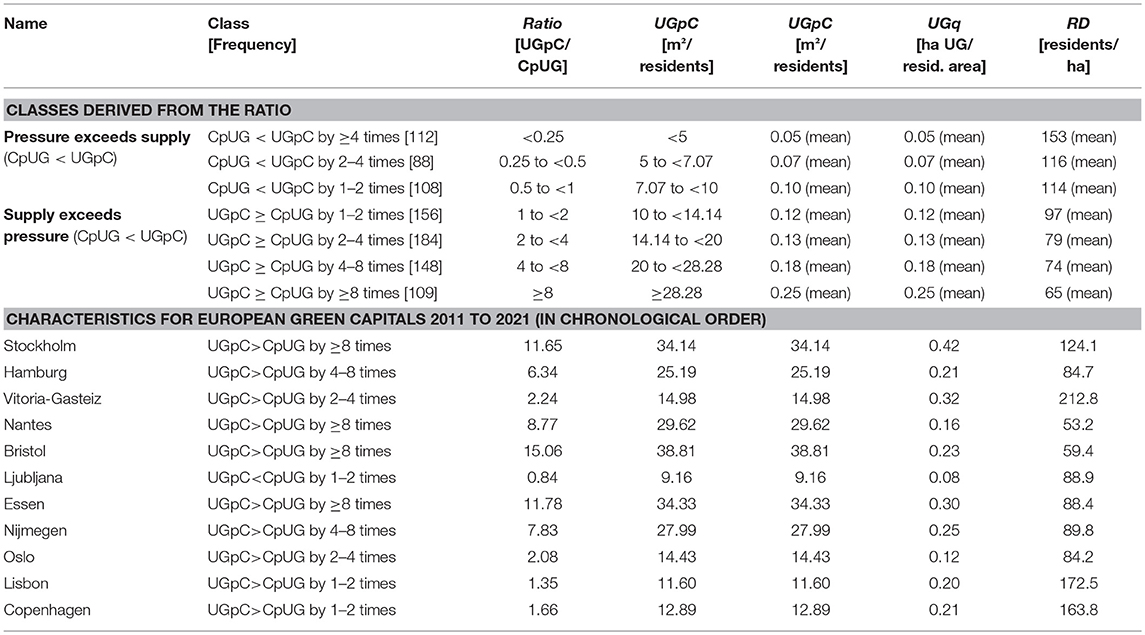
Table 1. Classes derived from the ratio between green space supply and green space pressure (top) and characteristics for European Green Capitals 2011 to 2021 (down).

Balancing Green Space Supply and Green Space Pressure for UG

The way cities in Europe actually balance green space supply and pressure is displayed in Figure 6 which contrasts the green space provision with the residential area for each of the seven classes.

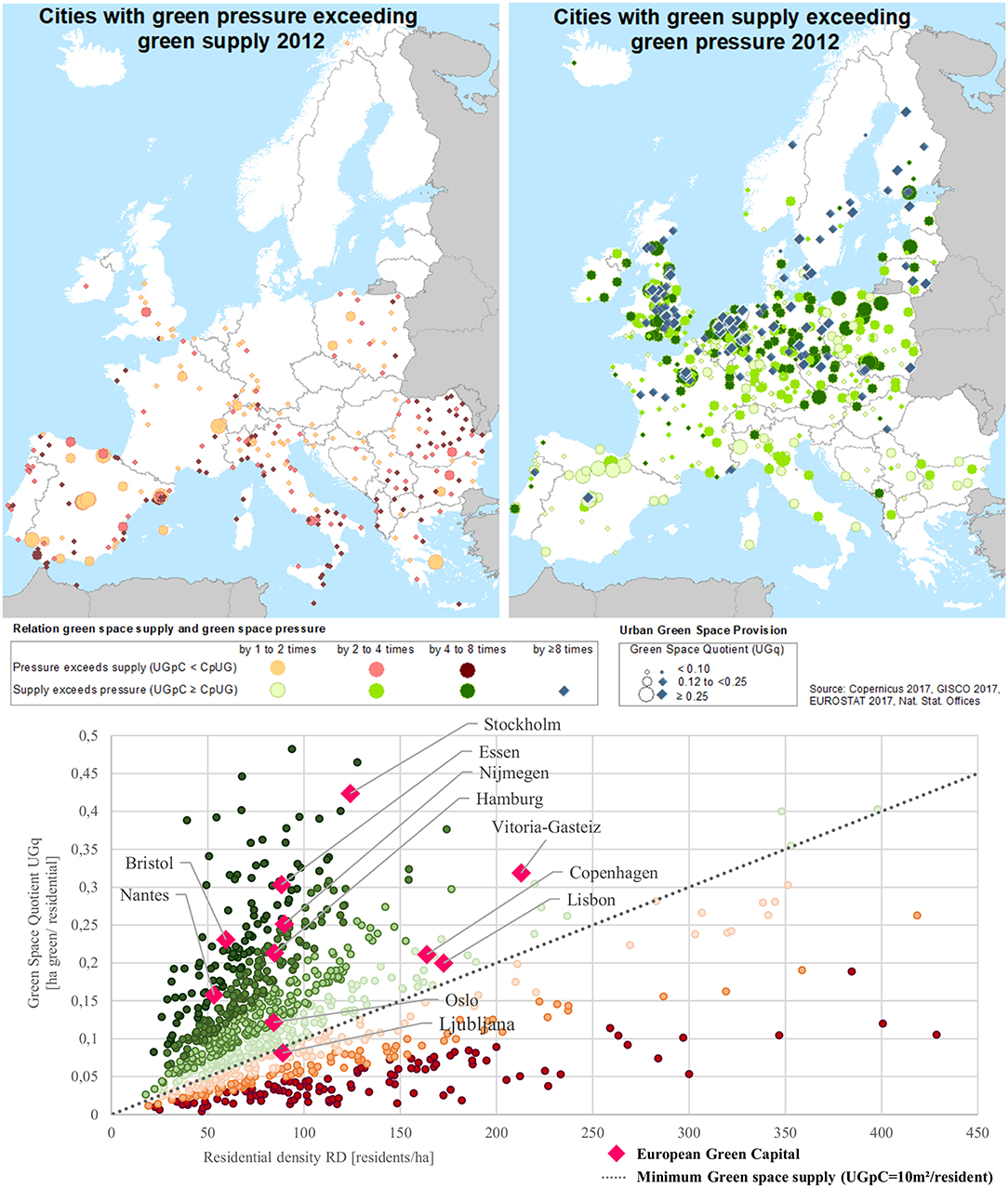
Figure 6. Seven classes for balancing green supply and pressure under different residential densities (RD) and green space provision (UGq).

The majority of cities with green pressure exceeding green supply provide a small amount of green spaces with a UGq below 0.11 and are located at the Iberian Peninsula, Italy and the Balkans. In the case of small cities below 70,000 residents, UGq are particularly likely to be below 0.05. However, a considerable number of cities with green space pressure exceeding the supply could, in relation to their low residential density, provide more UG, for example, in Italy, France, the UK (Ashford), Poland (Bielsko-Biala), Norway (Tromsö) or Germany (Siegen). In contrast, high dense cities like Barcelona, Thessaloniki, Athens, Naples, Palermo, Tirana or Skopje provide a higher amount of UG with UGq values of more than 0.1 but the per capita supply is comparatively low, nevertheless.

There are also cities in Southern Europe and the Balkans where the supply exceeds the pressure. These have a low residential density, such as in the case of Massa or Santiago de Compostela, and/or provide a lot of UG, such as in the case of Podgorica, Bologna, or Vitoria-Gasteiz. Vitoria-Gasteiz, the European Green Capital of 2013, provides more than one third UG for each hectare residential area with an UGq value of 0.32 (Table 1). Figure 6 shows that the highest green space provision for UG in Southern Europe can be found in cities in Northern Spain and in the metropolitan area of Madrid. Cities with a high green space supply for UG is characteristic for cities north of the line Kosice-Bern-Brest with UGpC values between 10 and 28 m²/resident, like Figure 6 displays. This is basically due to the high green space provision with UGq values between 0.12 and 0.18 in these cities which mitigates the residential density (Table 1).

In particular, cities in which the green space supply exceeds the pressure by more than 8 times show the highest UGpC values of >28.28 m²/resident due to three reasons. First, these high UGpC values are a result of residential densities below the average of 65 residents/ha (Table 1) although the green space provision UGq is below 0.16, as in the case of Bruges, Aalborg, Knivsta, Aberdeen, Trondheim or the Green Capital of 2014, Nantes. Second, other low density cities such as Tampere, Lund, Siauliai, Frankfurt (Oder) or the Green Capital of 2015, Bristol, show a high green space provision above 0.22. Third, a high green space provision can also be measured in high density cities such as Tallinn, Praha, Groningen, and Duisburg. Stockholm, the first European Green Capital, provides 0.42 ha UG for each ha of residential area, which results in a high green space supply of 34 m²/resident (Table 1).

Since the green supply is the result of both green space provision and residential density, there is no single optimal residential density for maximizing the green space supply. However, testing for differences of the mean RD between the seven classes presented in Table 1 we found significant differences. Table S3 suggests that the three classes with a supply exceeding the pressure by more than 2 times are significantly different from the other classes. Consequently, the corresponding threshold of residential density is between the means of the class “UGpC ≥ CpUG by 2 to 4 times” and “UGpC ≥ CpUG by 1 to 2 times.” Assuming an equal distribution, the threshold would be 88 residents/ha (Table 1). Five European Green Capitals have a RD values around this threshold. Essen, for instance, managed to achieve a high green supply of 34 m²/resident by providing for each ha residential around 0.3 ha urban green space.

Discussion

This paper has added to previous studies on green spaces in Europe. It has extended the view by systematically distinguishing between green space types, contrasting green provision and residential density, and detecting turning points of green space supply.

The Impact of Green Space Types on the Supply

The analysis has shown that the measurement of green space supply by UGpC and TGpC can be used to derive conclusions for urban green space provision, supply and demand. By systematically mapping the classification of green space supply contrasted by residential density for 905 cities in 2012, we find both similarities and differences to previous studies.

First, we detect high green space supply values in Northern European cities and low values in cities in Southern Europe while Western and Eastern European cities share similar average values, confirming previous studies (Fuller and Gaston, 2009; Kabisch and Haase, 2013; Larondelle et al., 2014). Even lower are the values in cities at the Balkans, a blind spot in hitherto comparative analysis on urban green. We found a weak but significant correlation between the green space provision and population size of a city. Although, the impact of city size on the supply of UG is low, as suggested by Poelman (2016), it could be, nevertheless, one indication for successful implementation or preservation of urban green spaces, especially in larger cities. It is evident that the share of UG on TG is significantly higher the larger a city is while smaller cities tend to have a higher share of forest areas.

Secondly, there are major differences in terms of the green space type considered for green supply. The ecological character of cities varies depending on the diversity of green space types that provide ecosystem services. The parallel study of urban green spaces and forest areas allows conclusion on the different ecosystem services these green spaces provide such as cultural, recreational or mitigating services beneficial to both human well-being and nature (Haase et al., 2014; Ma and Haarhoff, 2015). Parks are maintained differently as forest areas and therefore have different green qualities and quantities, play a different role as recreational spaces or for biodiversity conservation, or carbon sequestration and storage, and have different capacities for supporting cooling, noise-reduction and air filtration of pollutants (Haase, 2016). When taking into account forest (including woody) areas in addition to urban green spaces (TG) the clear North-South-divide mentioned above is partly masked and we find a much more scattered spatial pattern of the green space supply in Europe. While cities in Southern Europe and the Balkan still report the lowest average values, cities in these regions north of the line Porto (Portugal) and Varna (Bulgaria) report comparable higher supply rates when taking into account forest areas. In contrast, congested agglomerations, e.g., in the UK or the Benelux countries lack of forest areas and subsequently report lower supply values. While in large and dense cities urban green play an increasing role in the green supply (Kabisch and Haase, 2013), the role of forest areas is more decisive for the green space supply the smaller and less dense a city is. This is why the supply values for TG are higher for countries with a high share of small and medium sized cities such as France, Germany, Italy, and Spain.

Third, we mapped a large sample of European cities by systematically contrasting classes of residential density with classes of supply for two green space types. In line with Fuller and Gaston (2009), we find a lower total green space supply with increasing residential density. Contrary to their study but in line with Kabisch and Haase (2013), however, we found a weak but significant correlation between the green space provision and residential density and, even stronger, with population size of a city. Our relation is, however, weaker as Kabisch and Haase (2013) reported as we used residential density comparable to the approach by Fuller and Fuller and Gaston (2009). The classification for UG and TG confirms the correlation analysis: the majority of high density cities exhibit below average supply while the majority of low density cities tend to display an above average supply. This relation is even more obvious for TG than for UG. In contrast, in more than one third of cities the green space supply is higher than their residential density would suggest. This covers several capitals and larger cities as well as smaller cities in economically advanced or touristic attractive regions. In contrast, one fifth of European cities have lower supply values although their residential density is comparatively low. The share is almost the same between UG and TG affecting almost the same cities from the UK toward the Benelux countries, Paris, Western Germany to Northern Italy. Additionally, several other cities along the Mediterranean coastal regions as well as cities in Romania and Serbia have the potential to increase their green supply considering their residential density. These cities are paradigmatic for a lack or loss of the green network at the edge of the city, particularly high-density cities, which impacts forested areas and is in line with the prevailing discussion of the spatial impacts of urbanization (Kasanko et al., 2006; Nilsson and Ioannidis, 2014; Hedblom et al., 2017). The denser a city the lower is the share and supply of TG. In contrast, urban parks are less affected by being built over in contrast to e.g., farmland due to planning regulations and legal protection. Even newly created urban parks emerge as they have an aesthetic value for neighborhoods, and even an impact on real estate and property values in cities (Czembrowski and Kronenberg, 2016; Liebelt et al., 2018).

Turning Points in Green Space Supply

The combined perspective of green space supply, pressure and provision has shown that the two green spaces types UG and TG follow different logics when related to residential density. While the supply of TG is monotonous decreasing with increasing residential density the supply of UG indicates a turning point and, when contrasted with the indicator green space pressure for UG, a cutting point in which the pressure exceeds the supply. This cutting point was derived from the WHO criteria of 9 m²/resident which is widely used as the minimum standard for green space supply (WHO, 2012): at a value of 10 m²/resident the green space supply and pressure are equal (rounded in order to simplify the formula symbol for the green space pressure which was defined as residents/100 m²). Consequently, this cutting point indicates that the pressure on GS is so high that the supply becomes insufficient, and at the same time, represent the minimum value of the WHO criteria. It needs to be mentioned that the values scatter among European cities. Thus, the values for the cutting and turning point refer to the average trend curve of the data sample.

In order to demonstrate how cities balance green space supply and pressure, the paper has developed a systematic perspective, illustrated in Figure 6, which displays the UGpC value of a given combination of green space provision and residential density. When residential densities are too high, the green space supply significantly drops as more people use UG. Around a residential density of 140 residents/ha, this pressure exceeds the green space supply and leads to crowded parks and overuse. A decreasing green space provision due to residential constructions additionally increase the pressure on the remaining green spaces (Hedblom et al., 2017). This analysis has further demonstrated that the pressure on green spaces is higher when a city is larger in population size and when green space supply cannot be compensated for by additional green such as forest areas. Consequently, high residential densities with large areas of impervious surfaces limit the capacity of regulating and cultural ecosystem services such as air temperature lowering, air pollutant fixation or recreation with potential negative impacts on human health (Larondelle et al., 2014). Even more important is the fact that land use conflicts or pressures on the land from urban development will increase when cities grow and become more dense (Wolff et al., 2017). This is because competing interests, such as residential or greening purposes, need to be balanced (De Sousa, 2003; Haase, 2008; Herrmann et al., 2016).

Keeping green space supply stable under construction pressure in areas of high residential densities stable is a major task for planning (Westerink et al., 2013). A high supply of total green spaces can be achieved in both less dense and high density cities, in cities with a high and low green space provision. However, the higher the green space provision under a certain residential density the lower is the green space pressure (CpUG) and the higher is the green space supply (UGpC). Findings from this paper suggest that there is no single optimal residential density for which green supply can be maximized. According to the trend curve and contrasted with the data sample the urban green space supply is in particular high in cities with residential densities between 60 and 90 residents/ha. This residential density can be regarded as turning point from which the UGpC value decreases. A turning point at around 70 residents/ha is comparable low taking into account dense neighborhoods which are typical for large parts of Europe. Consequently, the turning point should not be taken as a target value or standard as it does aim to indicate the environmental situation of certain neighborhoods. Referring to the city scale and comparing a sample of 905 European cities indicates, however, that in a range between 60 and 80 residents/ha the urban green space supply is decreasing because (a) the supply is compensated by forest areas for cities with a lower residential density; and (b) the pressure on urban green space is increasing in cities with higher residential densities. In particular, the latter need to strike the balance between sustainability and liveability with regards to urban green space (Daw et al., 2016; Reyers and Selomane, 2018). However, it is up to further investigations to what extent these high densities indicate a decrease in the environmental quality—the indicators presented here serve as proxies in this regard.

Our results clearly indicate that turning points are different between cities of different density and location in Europe and between different types of neighborhoods within cities. Therefore, instead of overall urban standards of green supply across the whole city including core and periphery areas, different optimum values need to be defined sensitive to these characteristics. Using the European Green Capitals as showcases we have demonstrated that a high green space supply can be archived in cities with a low green space provision as long as residential density is low, like in Nantes, France. Stockholm, Sweden, is a contrasting example with a high residential density but also with a high green space provision. The two upcoming Green Capitals Lisboa (Portugal) and Copenhagen (Denmark) also show comparable high residential densities—however, the green spaces they provide is almost half of what Stockholm (Sweden) provides. Of course we find green spaces in dense cities better accessible compared to those in low residential density cities due to shorter commuting distances and a higher number of residents who are able to reach large central public parks. But dense cities need to find answers for an increasing pressure on existing green spaces in order not to go beyond the turning point after which urban green space declines.

Reflection of the Approach and Avenues for Further Research

The paper was designed as a comparative study systematically mapping the relation between residential density and green space supply for a large sample of cities. Although it has differentiated between types of green, the analysis only displays the green space classes available in the European Urban Atlas database (Copernicus, 2018) facing three limitations.

First, the green space database does not distinguish between green of different ownership, maintenance, accessibility etc. Accessible green spaces have been defined by geographical distance of 300 m and are assumed to be potentially accessible in line with previous studies (Handley et al., 2003; Kabisch et al., 2016; Poelman, 2016; Wüstemann et al., 2017). However, these areas can be private or not accessible due to other reasons while the database neglects smaller green spaces which might be accessible. Still, we use a homogenous and robust data set with a high resolution of 0.25 hectare, which allows us to produce results that are easy to communicate (EEA, 2011) as Urban Atlas is the only land-use data that allows a pan-European analysis, the assessment of different green types and, for further studies, the detection of changes in land-use over time.

Second, this paper used indicators that display the potential use and pressure of green spaces. While per capita green space is a widely accepted indicator green space pressure was designed for this study in a way that it indicates a cutting point when combined with green space supply and at the same time display the WHO criteria for a minimum green space supply (WHO, 2012). This follows previous conceptual and empirical studies on pressure on green spaces and ecosystems (Villamagna et al., 2013; Tan and Samsudin, 2017). However, as the conceptualization of the cutting point is rather explorative and has been designed for a larger sample, case studies need to re-question that the pressure on green spaces is really getting so high that supply becomes insufficient.

Third, the study uses quantitative indicators which measure the performance on the city level in line with previous studies on green spaces in Europe (Fuller and Gaston, 2009; Kabisch and Haase, 2013; Kabisch et al., 2016; Poelman, 2016). However, the study did not analyse the underlying green space strategies and planning approaches nor does it reflect trends and structures within the cities. Instead, we analyzed the variation of green space supply in Europe and contrasted the results with the values of European Green Capitals. European Green Capitals are awarded based on twelve common quantitative and qualitative environmental indicators, including the provision with urban green space. Using them as benchmark provides linkages to the high quality of life in these cities and the underlying green space strategies. This, in turn, can add to the prevailing discussion of balancing sustainability and liveability in cities (Villamagna et al., 2013; Daw et al., 2016).

In following studies, our findings may be further corroborated or disproved by applying a more nuanced analysis to:

• Analyse changes of green space supply with changing residential density over time and population growth in order to detect long terms effects.

• Focus on green spaces and using certain parameters such as the distance independent of administrative boundaries in order to detect the role of the city's hinterland for the green space supply in cities.

• Apply the concept of turning and cutting points to a more differentiated dataset of green spaces in order to develop a better understanding of accessible green spaces and apply it to different spatial scales such as neighborhoods.

• Question to what extend a high provision with UG in prosperous cities is a result of the ability and financial resources to priorities green infrastructures and the result of successful or failed green space planning (Herrmann et al., 2016).

• Further conceptualize turning points to be used in green space research (Reyers and Selomane, 2018) in order to define different optimum values.

Conclusions

For most of the European cities a decrease of urban population or built-up area in the future cannot be expected (UN, 2018; Wolff et al., 2018). Consequently, finding a balance between residential density, a high liveability in a green and sustainable urban environment is a major challenge for urban planning. By systematically understanding the quantitative linkages between green spaces in cities and densities, this paper helps to respond to the growing need for better urban land management at city level and to secure scarce open land and natural resources within cities (Herrmann et al., 2016). In particular, we claim for two points.

First, we need a perspective which does not just take the green provision into account but allows a combined perspective of pressure and supply. The policies of the EU promote multifunctional green spaces as green infrastructure or nature-based solutions in order to foster the sustainable development of cities (Biodiversity Strategy; EC, 2011, whereas the demand perspective in terms of densities was largely neglected. However, it is important that the provision of green spaces and the planning of and for high residential densities go hand in hand Pauleit et al., 2005; Cheng, 2009). Thereby, indicators of green space supply and pressure can be used in order to reflect one quantitative facet of human-environmental relations addressing the multi-functionality of green spaces in cities.

Second, planners and scholars are asked to increasingly account for the complexity of green space accessibility to existing green spaces, the green space potential of the hinterland (Westerink et al., 2013; Larondelle et al., 2014; Herrmann et al., 2016; Xu et al., 2018). In particular, the variation detected in terms of regional location and population size suggest that a given green space provision does not necessarily lead to a similar green space supply what requires contextualized strategies. Therefore, contextualized strategies for green space planning should take into account turning and cutting points in green space supply of the regional green infrastructure and their implications. The assessment of robust and comparative data on green spaces for a large sample of European cities in this paper can be used as a comparative information in this regard (UN, 2015). Therefore, this paper argues that the compact city model should not be applied without considering different needs of density variations, and aligning these needs with the quantity, quality and ecosystem service capacities of green spaces.

Author Contributions

MW and DH conceived and designed the study. MW collected and processed data and performed statistical and spatial analysis, both authors contributed to writing.

Conflict of Interest Statement

The authors declare that the research was conducted in the absence of any commercial or financial relationships that could be construed as a potential conflict of interest.

The reviewer SP declared a past collaboration with one of the authors DH to the handling Editor.

Acknowledgments

This research was carried out as part of the project ENABLE, funded through the 2015–2016 BiodivERsA COFUND call for research proposals, with the national funders The Swedish Research Council for Environment, Agricultural Sciences, and Spatial Planning, Swedish Environmental Protection Agency, German Aeronautics and Space Research Center, National Science Center (Poland), The Research Council of Norway and the Spanish Ministry of Economy and Competitiveness.

Supplementary Material

The Supplementary Material for this article can be found online at: https://www.frontiersin.org/articles/10.3389/fenvs.2019.00061/full#supplementary-material

References

Beninde, J., Veith, M., and Hochkirch, A. (2015). Biodiversity in cities needs space: a meta-analysis of factors determining intra-urban biodiversity variation. Ecol. Lett. 18, 581–592. doi: 10.1111/ele.12427
Burkhard, B., Kroll, F., Nedkov, S., and Müller, F. (2012). Mapping ecosystem service supply, demand and budgets. Ecol. Indic. 21, 17–29. doi: 10.1016/j.ecolind.2011.06.019
Burton, E. (2000). The compact city: just or just compact? A preliminary analysis. Urban Stud. 37, 1969–2001. doi: 10.1080/00420980050162184
Cheng, V. (2009). “Understanding density and high density,” in Designing High-Density Cities: for Social and Environmental Sustainability, ed E. Ng (London: Earthscan), 3–17.
Cleveland, W. S. (1981). A program for smoothing scatterplots by robust locally weighted fitting. Am. Stat. 35:54. doi: 10.2307/2683591
Commission of European Communities (1990). Green Paper on the Urban Environment – Communication From the Commission to the Council and the Parliament. EUR 12902. Brussels: EC.
Copernicus (2018). Urban Atlas 2006 and 2012. Available online at: https://land.copernicus.eu/local/urban-atlas (accessed September 8, 2017).
Copernicus (2019). Corine Land Cover 2000 and 2018. Available online at: https://land.copernicus.eu/pan-european/corine-land-cover (accessed February 15, 2019).
Czembrowski, P., and Kronenberg, J. (2016). Hedonic pricing and different urban green space types and sizes: insights into the discussion on valuing ecosystem services. Landsc. Urban Plan. 146, 11–19. doi: 10.1016/j.landurbplan.2015.10.005
Daw, T. M., Hicks, C., Brown, K., Chaigneau, T., Januchowski-Hartley, F., Cheung, W., et al. (2016). Elasticity in ecosystem services: exploring the variable relationship between ecosystems and human well-being. Ecol. Soc. 21:11. doi: 10.5751/ES-08173-210211
De Sousa, C. A. (2003). Turning brownfields into green space in the City of Toronto. Landsc. Urban Plan. 62, 181–198. doi: 10.1016/S0169-2046(02)00149-4
Duany, A., Plater-Zyberk, E., and Speck, J. (2001). Suburban Nation. New York, NY: North Point Press.
EC (2011). Our Life Insurance, Our Natural Capital: An EU Biodiversity Strategy to 2020. COM(2011)244. Brussels: Communication from the commission to the European parliament, the council, the economic and social committee and the committee of the regions.
EC (2019). European Green Capital. Winning Cities. Available online at: http://ec.europa.eu/environment/europeangreencapital/ (accessed February 20, 2019).
EEA (2011). Green Infrastructure and Territorial Cohesion. The Concept of Green Infrastructure and its Integration Into Policies Using Monitoring Systems. EEA Technical report No 18/2011.
EEA (2017). Landscapes in Transition an Account of 25 Years of Land Cover Change. EEA Report No 10/2017, European Environment Agency.
EG (2018). Urban Audit 2011-2014. Available online at: https://ec.europa.eu/eurostat/web/gisco/geodata/reference-data/administrative-units-statistical-units (accessed February 8, 2018).
Elmqvist, T., Redman, C. L., Barthel, S., and Costanza, R. (2017). “History of urbanization and the missing ecology,” in Urbanization, Biodiversity and Ecosystem Services: Challenges and Opportunities, eds T. Elmqvist, M. Fragkias, J. Goodness, B. Güneralp, P. J. Marcotullio, R. I. McDonald, et al. (Dordrecht; Heidelberg; New York, NY; London: Springer), 13–30.
ESPON (2014). ESPON 2013 Database Dictionary of Spatial Units. Nomenclature of WUTS (World Unified Territorial System).
EUROSTAT (2018). Urban Audit Database – Cities and Greater Cities. Available online at: https://ec.europa.eu/eurostat/web/cities/data/database (accessed November 7, 2017).
Fuller, R. A., and Gaston, K. J. (2009). The scaling of green space coverage in European cities. Biol. Lett. 5, 352–355. doi: 10.1098/rsbl.2009.0010
Grimm, N. B., Faeth, S. H., Golubiewski, N. E., Redman, C. L., Wu, J., Bai, X., et al. (2008). Global change and the ecology of cities. Science 319, 756–760. doi: 10.1126/science.1150195
Haase, D. (2008). Urban ecology of shrinking cities: an unrecognized opportunity? Nat. Cult. 3, 1–8. doi: 10.3167/nc.2008.030101
Haase, D. (2016). “Was leisten Stadtökosysteme für die Menschen in der Stadt?” in Stadtökosysteme Funktion, Management und Entwicklung, eds J. Breuste, S. Pauleit, D. Haase, and M. Sauerwein (Berlin; Heidelberg: Springer Berlin Heidelberg), 129–163.
Haase, D., Larondelle, N., Andersson, E., Artmann, M., Borgström, S., Breuste, J., et al. (2014). A quantitative review of urban ecosystem service assessments: concepts, models, and implementation. Ambio 43, 413–433. doi: 10.1007/s13280-014-0504-0
Hall, P. (2001). “Sustainable cities or town cramming?” in Planning for a Sustainable Future, eds A. Layard, S. Davoudi, and S. Batty (London: Spon), 101–114.
Handley, J., Pauleit, S., Slinn, P., Barber, A., Baker, M., Jones, C., et al. (2003). Accessible Natural Green Space Standards in Towns and Cities: A Review and Toolkit for Their Implementation. English nature research reports, 526.
Hansen, R., Rolf, W., Santos, A., Luz, A. C., Száras, L., Tosics, I., et al. (2016). Advanced Urban Green Infrastructure Planning and Implementation - Innovative Approaches and Strategies from European Cities. Deliverable 5.2. GREEN SURGE report. Available online at: https://greensurge.eu/working-packages/wp5/files/D5_2_Hansen_et_al_2016_Advanced_UGI_Planning_and_Implementation_v3.pdf (accessed February 5, 2019).
Hedblom, M., Andersson, E., and Borgström, S. (2017). Flexible land-use and undefined governance: from threats to potentials in peri-urban landscape planning. Land Use Policy 63, 523–527. doi: 10.1016/j.landusepol.2017.02.022
Herrmann, D. L., Schwarz, K., Shuster, W. D., Berland, A., Chaffin, B. C., Garmestani, A. S., et al. (2016). Ecology for the shrinking city. Bioscience 66, 965–973. doi: 10.1093/biosci/biw062
Jabareen, J. R. (2006). Sustainable urban forms: their typologies, models, and concepts. J. Plan. Educ. Res. 1, 38–52. doi: 10.1177/0739456X05285119
Kabisch, N., and Haase, D. (2013). Green spaces of European cities revisited for 1990-2006. Landsc. Urban Plan. 110, 113–122. doi: 10.1016/j.landurbplan.2012.10.017
Kabisch, N., Qureshi, S., and Haase, D. (2015). Human–environment interactions in urban green spaces—a systematic review of contemporary issues and prospects for future research. Environ. Impact Assess. Rev. 50, 25–34. doi: 10.1016/j.eiar.2014.08.007
Kabisch, N., Strohbach, M., Haase, D., and Kronenberg, J. (2016). Urban green space availability in European cities. Ecol. Indic. 70, 586–596. doi: 10.1016/j.ecolind.2016.02.029
Kasanko, M., Barredo, J. I., Lavalle, C., McCormick, N., Demicheli, L., Sagris, V., et al. (2006). Are European cities becoming dispersed? Landsc. Urban Plan. 77, 111–130. doi: 10.1016/j.landurbplan.2005.02.003
Kowarik, I. (2011). Novel urban ecosystems, biodiversity, and conservation. Environ. Pollut. 159, 1974–1983. doi: 10.1016/j.envpol.2011.02.022
Larondelle, N., Haase, D., and Kabisch, N. (2014). Mapping the diversity of regulating ecosystem services in European cities. Glob. Environ. Chang. 26, 119–129. doi: 10.1016/j.gloenvcha.2014.04.008
Liebelt, V., Bartke, S., and Schwarz, N. (2018). Hedonic pricing analysis of the influence of urban green spaces onto residential prices: the case of Leipzig, Germany. Eur. Plan. Stud. 26, 133–157. doi: 10.1080/09654313.2017.1376314
Ma, J., and Haarhoff, E. (2015). “The GIS-based research of measurement on accessibility of green infrastructure - a case study in Auckland,” in MIT CUPUM Conference Proceeding, The 14th International Conference on Computers in Urban Planning and Urban Management, July 7-10 (Cambridge, MA: MIT Press).
Masnavi, M. (2000). “The new millennium and the new urban paradigm: The compact city in practice,” in Achieving Sustainable Urban Form, eds K. Williams, E. Burton, and M. Jenks (New York, NY: Spon), 64–74.
Masnavi, M. R. (2007). Measuring urban sustainability: developing a conceptual frameworkfor bridging the gap between theoretical levels and operational levels'. Int. J. Environ. Res. 1, 188–197. doi: 10.22059/IJER.2010.125
McPhearson, T., Haase, D., Kabisch, N., and Gren, Å. (2016). Advancing understanding of the complex nature of urban systems. Ecol. Indic. 70, 566–573. doi: 10.1016/j.ecolind.2016.03.054
Mell, I. (2015). “Green infrastructure planning: policy and objectives,” in Handbook on Green Infrastructure: Planning, Design and Implementation, eds D. Sinnett, N. Smith, and S. Burgess (Cheltenham: Edward Elgar Publishing), 105–123.
Netherlands Presidency (2016). Urban Agenda for the EU: Pact of Amsterdam. Factsheet. Available online at: https://agendastad.nl/wp-content/uploads/2015/02/EU-Urban-Agenda-factsheet.pdf (accessed June 15, 2018).
Neumann, M. (2005). The compact city fallacy. J. Plan. Educ. Res. 25, 11–26. doi: 10.1177/0739456X04270466
Nilsson, K. J., and Ioannidis, P. G. (2014). Strategies for sustainable urban development and urban-rural linkages. Eur. J. Spatial Dev. 55, 1–26.
OSM (2019). OSM Admin Boundaries Map 4.4.6. Available online at: https://wambachers-osm.website/boundaries/ (accessed February 13, 2019).
Pauleit, S., Ennos, R., and Golding, Y. (2005). Modeling the environmental impacts of urban land use and land cover change - a study in Merseyside, UK. Landsc. Urban Plan. 71, 295–310. doi: 10.1016/j.landurbplan.2004.03.009
Poelman, H. (2016). A Walk to the Park?—Assessing Access to Green Urban Areas in Europe's Cities. Working Paper 01/2016, European Commission, Brussels.
Reyer, M., Fina, S., Siedentop, S., and Schlicht, W. (2014). Walkability is only part of the story: walking for transportation in Stuttgart, Germany. Int. J. Environ. Res. Public Health 11, 5849–5865. doi: 10.3390/ijerph110605849
Reyers, B., and Selomane, O. (2018). “Social-ecological systems approaches Revealing and navigating the complex trade-offs of sustainable development,” in Ecosystem Services and Poverty Alleviation: Trade-offs and Governance, eds K. Schreckenberg, G. Mace, and M. Poudyal (London: Routledge), 39–54.
Rouse, D. C., and Bunster-Ossa, I. F. (2013). Green Infrastructure: A Landscape Approach. Planning Advisory Service Report 571, Chicago, IL: American Planning Association. Available online at: https://planning.org/publications/report/9026895 (accessed december 15, 2018)
Talgorn, B., Audet, C., Le Digabel, S., and Kokkolaras, M. (2018). Locally weighted regression models for surrogate-assisted design optimization. Optimiz. Eng. 19, 213–238. doi: 10.1007/s11081-017-9370-5
Tan, P. Y., and Samsudin, R. (2017). Effects of spatial scale on assessment of spatial equity of urban park provision. Landsc. Urban Plan. 158, 139–154. doi: 10.1016/j.landurbplan.2016.11.001
UN (2015). Transforming our World: The 2030 Agenda for Sustainable Development. Resolution A/RES/70/1, Seventieth session United Nations General Assembly, Agenda items 15 and 116.
UN (2018). World Urbanization Prospects: the 2018 Revision. New York, NY: United Nations, Department of Economic and Social Affairs, Population Division.
Villamagna, A. M., Angermeier, P. L., and Bennett, E. M. (2013). Capacity, pressure, demand, and flow: a conceptual framework for analyzing ecosystem service provision and delivery. Ecol. Complex. 15, 114–121. doi: 10.1016/j.ecocom.2013.07.004
Weber, N., Haase, D., and Franck, U. (2014). Traffic-induced noise levels in residential urban structures using landscape metrics as indicators. Ecol. Indic. 45, 611–621. doi: 10.1016/j.ecolind.2014.05.004
Westerink, J., Haase, D., Bauer, A., Ravetz, J., Jarrige, F., and Aalbers, C. B. E. M. (2013). Dealing with sustainability trade-offs of the compact city in peri-urban planning across European city regions. Eur. Plan. Stud. 21, 473–497. doi: 10.1080/09654313.2012.722927
WHO (2012) Health Indicators of Sustainable Cities in the Context of the Rio+20 UN Conference on Sustainable Development. WHO/HSE/PHE/7.6.2012f 2012.
Wiersinga, W. (1997). Compensation as a Strategy for Improving Environmental Quality in Compact Cities. Amsterdam: Bureau SME.
Wolff, M., Haase, A., Haase, D., and Kabisch, N. (2017). The impact of urban regrowth on the built environment. Urban Stud. 54, 2683–2700. doi: 10.1177/0042098016658231
Wolff, M., Haase, D., and Haase, A. (2018). Less dense or more compact? Discussing a density model of urban development for European urban areas. PLoS ONE. 13:e0192326. doi: 10.1371/journal.pone.0192326
Wüstemann, H., Kalisch, D., and Kolbe, J. (2017). Access to urban green space and environmental inequalities in Germany. Landsc. Urban Plan. 164, 124–131. doi: 10.1016/j.landurbplan.2017.04.002
Keywords: green space supply, residential density, turning points, European cities, comparative analysis
Citation: Wolff M and Haase D (2019) Mediating Sustainability and Liveability—Turning Points of Green Space Supply in European Cities. Front. Environ. Sci. 7:61. doi: 10.3389/fenvs.2019.00061
Received: 10 December 2018; Accepted: 23 April 2019;
Published: 14 May 2019.
Edited by:
Ioan Cristian Ioja, University of Bucharest, RomaniaReviewed by:
Mihai Razvan Nita, University of Bucharest, RomaniaStephan Pauleit, Technische Universität München, Germany
Copyright © 2019 Wolff and Haase. This is an open-access article distributed under the terms of the Creative Commons Attribution License (CC BY). The use, distribution or reproduction in other forums is permitted, provided the original author(s) and the copyright owner(s) are credited and that the original publication in this journal is cited, in accordance with accepted academic practice. No use, distribution or reproduction is permitted which does not comply with these terms.
*Correspondence: Manuel Wolff, manuel.wolff@geo.hu-berlin.de