Research on the method of predicting CEFR core thermal hydraulic parameters based on adaptive radial basis function neural network

1 Introduction

Reactor thermal hydraulic parameters, such as the maximum fuel sheath surface temperature, are closely related to the economics and safety of nuclear power plants. Accurately predicting the change trend of key thermal hydraulic parameters of reactors under various working conditions in a short time can enable operators and nuclear power plant systems to respond in advance, significantly improve the reactor safety, and effectively prevent nuclear power plant accidents. However, during reactor operation, the key thermal hydraulic parameters are affected by multiple physical quantities simultaneously and their change trends are complex; thus, it is difficult for adaptive forecasting methods to achieve accurate forecasts in a short time. Therefore, for improving reactor security, it is vital to develop a new forecasting method for the key thermal hydraulic parameters of reactors.

Neural network is a mathematical model that simulates the behavioral characteristics of animal neurons for information processing. Owing to its nonlinear, large-scale, strong parallel processing ability, robustness, fault tolerance, and strong self-studying ability, it has been triumphantly applied in many domains, such as nonlinear function approximation, information classification, type recognition, information processing, image-processing, control and hitch diagnosis, financial forecast, time series forecasting (Liang and Wang, 2021). Since the 1990s, many studies have made use of various neural network arithmetics to forecast core parameters. Huang et al. (2003) made use of the back propagation (BP) artificial neural network to forecast the critical heat flux density of reactors. Compared with the traditional method, this method exhibits a high forecasting accuracy and is more convenient to update and use, thereby making it easier to adopt. Taking the 10 MW high temperature gas-cooled reactor into consideration, Li et al. (2003) monitored and analyzed the changes in various parameters of reactors under various faults by using an artificial neural network. Mohamedi et al. (2015) used a neural network to predict the effective multiplication factor Keff and peak fuel power Pmax of a light water reactor; their results indicate a high forecasting accuracy, while demonstrating that the neural network analysis method can largely cut down the time acquired for this optimization process. Peng et al. (2014) proposed that the normalized adaptive radial basis function (RBF) neural network arithmetic can be used for accurately reconstructing the axial power array of the core; they also studied the power array of the ACP-100 modular reactor. Their study also found that this technique exhibits sufficient robustness to overcome the intrinsic ill-posedness during power array reconstruction. However, most of the existing studies are based on the widely used BP neural network, and rarely involve other neural networks. Furthermore, most of the current research focuses on forecasting and analyzing steady-state parameters of reactors. However, there are few studies on the transient-state condition, which significantly affects reactor security; therefore, forecasting its change trends is more important. Based on the adaptive RBF neural network, this study forecasts the maximum surface temperature of the fuel sheath of a reactor under steady-state and transient-state conditions, compares the adaptive RBF neural network with the widely used adaptive BP neural network, and elucidates the adaptability of the adaptive RBF neural network for forecasting key parameters.

2 Introduction of neural network model

2.1 Back propagation neural network

The traditional BP neural network is a feed forward neural network based on the error BP arithmetic (Huang et al., 2003). It simulates the reactive procedure of human brain neurons to external stimulus signals, constructs a multi-layer perceptron model, and adopts forward propagation and error backpropagation (Liang and Wang, 2021). Through multiple iterative studies, this neural network can describe numerous input-output pattern mappings without revealing their specific mathematical equations, and can successfully build an intelligent model for solving nonlinear data (Liang and Wang, 2021). As one of the mostly widely applied neural networks, its modeling process mainly includes forward transmission of information and error BP (Lyu et al., 2021). The traditional BP neural network has a simple construction and stable gradient descent. In theory, it can realize high-precision nonlinear fitting. Moreover, it can be utilized in the nonlinear function approach, time series forecasting, and other applications.

The traditional BP neural network is an arithmetic comprising an input layer, an output layer, and a hidden layer. The input and output layers are sufficiently connected, and there are no connections between neurons in the same layer (Li et al., 2003). Figure 1 shows the topology of a typical BP neural network. The input dimension is l, number of hidden layer nodes is p, and output dimension is q.

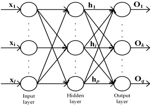
FIGURE 1. Structure of the 3-layer BP neural network.

The traditional BP neural network is studied via a two-step procedure: forward propagation of signals and BP of signals (Huang et al., 2003). First, the input signal is transmitted through the input layer, hidden layer, and output layer (in that order) to complete the forward propagation of the signal. When the signal error of the output layer is larger than the anticipated error, the error BP process is performed. Second, the error values obtained via calculation are used to modify the weights of each layer one by one, and BP is carried out from the output layer to the hidden and input layers. Finally, through continuous forward propagation of signals and BP of errors, weights of each layer are continuously modified. This procedure is iterated until either the signal error of the output layer decreases to a tolerable level, or the pre-determined number of iterations is reached.

According to the three-layer BP neural network method, the following presumptions are made: the input vector is $X={\left(x_1,x_2,...,x_i,...,x_l\right)}^T$; output vector of the hidden layer is $H={\left(h_1,h_2,...,h_j,...,h_p\right)}^T$; output vector is $O={\left(o_1,o_2,...,o_k,...,o_q\right)}^T$; prospective output vector is $D={\left(d_1,d_2,...,d_k,...,d_q\right)}^T$; weight matrix between the input layer and the hidden layer is $W=\left(W_1,W_2,...,W_j,...,W_p\right)$ (Li et al., 2003); weight matrix between the hidden layer and output layer is $V=\left(V_1,V_2,...,V_k,...,V_q\right)$; Wj is the weight vector consistent with the jth neuron in the hidden layer; and Vk is the weight vector consistent with the kth neuron in the output layer (Li et al., 2003).

2.1.1 Forward propagation of signals

The following equations are associated with the hidden layer:

where netj is the input of the jth neuron in the hidden layer and f(x) is the transfer function.

The following equation is associated with the output layer:

After using the transfer function f(x) as the bipolar sigmoid function, we obtain the following expression:

The derivative of this function is:

2.1.2 Backward propagation of errors

The mean square error of the output is shown below:

By determining the gradient change of the loss function E with respect to each weight, the error is reversely transferred; this ensures that all the weights are adjusted in the direction in which the loss function E decreases the fastest. The loss function E can be continuously reduced, and the output constantly approaches the actual output value.

The network weight is updated as follows:

where $\eta$ is the studying rate, which is a constant in the adaptive gradient descent method.

The structure of the traditional BP neural network is relatively simple, and the gradient descent is relatively stable (Wang et al., 2020). Theoretically, this network can achieve high precision nonlinear fitting, while exhibiting a certain application value for nonlinear function approximation, time series forecasting, and other approaches. However, the studying rate of the traditional BP neural network does not change once initialized, which makes it difficult to implement the correct studying process at minimum loss function values, thereby leading to a low convergence speed. Thus, the adaptive moment estimation (Adam) arithmetic (such as the adaptive BP neural network) has been used to improve the gradient descent method (Wang et al., 2020), which ensures that the studying rate can adapt to changes in the size of the loss function to improve the convergence speed.

The Adam arithmetic parameters are updated as follows:

where $\theta$ is any parameter; $l{r}_t$ is the studying rate; $\epsilon$ is set as 10–8 to ensure that the division result is not 0; $t$ is the number of iterations: $\overline{m}$ is the bias-corrected initial moment evaluation; and $\overline{v_t}$ is the bias-corrected second moment evaluation (Wang et al., 2020). Figure 2 indicates the calculation flow diagram of the neural network forecast method used in this study.

FIGURE 2. Flow-process diagram of neural network forecast model.

2.2 Adaptive radial basis function neural network

The generation of RBF neural network has a strong biological background. In human cerebral cortex, local regulation and overlapping receptive fields are the distinguishing features of human brain response. Based on the characteristics of receptive fields, Moody and Darken established a model, namely: RBF network.

The RBF neural network is a local approximate feed forward neural network, which can approach any nonlinear function. It exhibits an optimum generalization capability and a rapid convergence speed, even when dealing with mechanisms that are difficult to analyze in the system. One of the most commonly used in the RBF neural network is the Gaussian Kernel Function, which has the best forecasting performance compared to other kernel functions such as Linear Kernel Function and Polynomial Kernel Function (Lou et al., 2013). Compared with that of the BP neural network, the RBF neural network exhibits a faster convergence speed because it comprises only one middle hidden layer. The hidden layer considers the Euclidean distance as an independent variable between the input vector and central vector, while utilizing the Gaussian Kernel Function as the activation function, which can map the data to infinite dimensions. If the input is at a considerable distance from the middle of the activation function, the output value of the hidden layer tends to be significantly small. A real mapping effect is observed only when the Euclidean distance is negligible, thereby demonstrating local approximation. Poggio and Girosi have demonstrated that generalized RBF neural networks exhibit superior performance for continuous function approximation and has great noise immunity (Maruyama and Girosi, 1992). Currently, Gaussian radial basis neural networks is one of the most common RBF neural networks. The network construction and the RBF neural network arithmetic tend to differ in these neural networks, which overcomes the shortcomings that BP network is easy to fall into local optimal solution and its convergence speed is slow to a certain extent (Hong et al., 2021). Figure 3 shows the basic structure of single output layer RBF neural network.

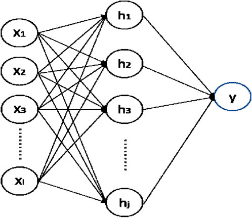
FIGURE 3. Structure of single output layer RBF neural network.

In this work, the Gaussian kernel function is selected as the RBF, which is controlled by the central location and relevant width parameters. The width of the function unit controls the decline rate of the function. The output of the hidden layer is represented as:

where $x-c_j$ is the Euclidean distance; $j$is the number of hidden layer nodes; $c_j$ and ${\sigma }_j$ are the central vector and distance of the jth node in the hidden layer, respectively; $h_j$ is the output of the jth node in the hidden layer; ${\omega }_j$is the weight of the jth neuron; and y is the output of the network. In this article, these parameters are optimized using the Adam arithmetic.

The specific implementation steps of the generalized RBF neural network are similar to the BP neural network, that is, after a single training, the gradient descent method is used to iterate the weights of each neuron, when the termination condition is reached, the iteration is stopped and a group of optimal weights are obtained. The generalized RBF neural network also has the problem of constant learning rate in the iterative process. Therefore, this study has optimized the weight update method of the generalized RBF neural network through adaptive gradient descent method to obtain the adaptive RBF neural network arithmetic.

From the above analysis, it can be seen that the adaptive RBF neural network has better generalization capability and faster convergence speed than the adaptive BP neural network, which makes it have a better application prospect in nonlinear time series forecasting. In view of this, the performance of adaptive BP neural network and adaptive RBF neural network applied to steady-state and transient analysis of key thermal hydraulic parameters of reactor core is studied below.

3 Comparative analysis of different neural network models

For comparing the advantages and disadvantages of different adaptive neural network models, the maximum surface temperature of a fuel rod sheath of the China Experimental Fast Reactor (CEFR) under different conditions is selected as the basis for comparison. The main dynamic thermal hydraulic parameters of CEFR are shown in Table 1. During the CEFR equilibrium cycle, the fuel power and reactor core flow rate of the fuel assembly are determined by referencing the CEFR safety analysis report. The specific values are shown in Figure 4, where the first line represents the sub channel number during the analysis of the 1/2 core model. The second line represents the power of the fuel assembly in kW, while the third line represents the coolant flow in kg/s.

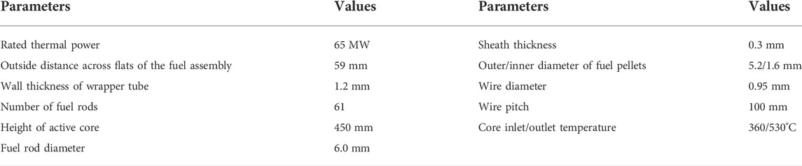
TABLE 1. Main parameters of CEFR.

FIGURE 4. Distribution of channel number, power, and flow rate for analysis of the 1/2 core model.

3.1 Steady-state single assembly analysis

The normal operating state of reactors is steady-state condition. In that case, the boundary conditions such as inlet and outlet temperature and flow rate change little, in order to simplify the model, which can be approximately considered as unchanged. Studying the trends of key thermal hydraulic parameters under steady-state conditions can further improve the reactor safety and economy. For studying the forecasting performance of two neural networks under steady-state conditions, the core model of CEFR is used to perform steady-state analysis, which can be divided into three parts: acquisition of data samples, determination of network topology, and result and analysis.

3.1.1 Acquisition of data samples

The CEFR core is divided into four fuel zones, with 61 fuel rods in each assembly. Figure 5 shows the 126 sub channels obtained by using the SUBCHANFLOW code (Gomez et al., 2012) when building the CEFR single-assembly model.

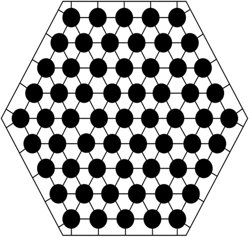
FIGURE 5. Number of coolant channels.

According to the CEFR safety analysis report, the channel power and flow range of CEFR is 0–1,200 kW and 0–6 kg/s, respectively. Several datasets are arbitrarily selected, combined with the main parameters of CEFR in Table 1, and used as SUBCHANFLOW input. After calculations are performed by the code, 1,000 significant dataset samples are obtained.

The generalization capability of the adaptive BP neural network is relatively poor, and the most intuitive performance of the generalization capability is the overfitting and under fitting, both of which are two states in the neural network training process. At the beginning of the training, the error of the training set and the test set is relatively poor, and the entire model is in the state of under fitting. With the increase of model complexity, the error of the training set and the test set will become smaller and smaller, the error of the test set will begin to rise after a certain demarcation point, and the entire model will enter the overfitting state. If the neural network training is stopped at the demarcation point, the generalization capability of the network will be best. Therefore, the generalization capability can be improved by introducing verification sets. Adding the validation set to the training network helps in determining the change in the forecast error at any time. When the error gradually decreases to the inflection point, the network training is stopped and the network weight can no longer be updated, which can avoid overfitting and under fitting of the model. Subsequently, the dataset is divided into two parts: training set (accounts for 80%) and the validation and test sets (account for 20%) (Yang et al., 2022); the number of samples in these two datasets is the same. Therefore, 800 datasets are randomly selected as the training samples, 100 are chosen as the verification samples, and the remaining 100 are used as the test samples. Since the adaptive RBF neural network exhibits optimum generalization capability and convergence speed, the training and test samples can be used directly in the ratio of 80 and 20%, respectively. Therefore, 800 datasets are stochastically chosen as the training samples, and the remaining 200 datasets are the test samples. The evaluation model is constructed by predicting the results of the test set. The training samples only participate in network training, and the test samples only participate in the forecasting process and result analysis. The training set is randomly disrupted before each training to avoid excessive recording of local features by the neural network.

3.1.2 Determination of network topology

The number of hidden layer nodes and hidden layers significantly affects the topology of neural networks. An excessive number of hidden layers tends to destabilize the network. An increasing trend in the number of hidden layers leads to an increased probability of local optimization in the training process. An excessive number of hidden layer nodes tends to affect the learning time of the network, while an extremely small number either leads to poor network learning or no learning at all. In addition, the number of hidden layer nodes and hidden layers is related to the generalization ability of the network (Li and He, 2006).

Nielson has theoretically proven that a neural network with one hidden layer can approach all functions that are continuous in a closed interval by changing the number of hidden layer nodes (Azghadi et al., 2007); consequently, a network with good performance can be obtained. Therefore, two different neural networks with a three-layer topology structure are chosen; that is, the number of hidden layers in these networks is one. The number of hidden layer nodes is continuously debugged by performing iterative calculations for each neural network, and the number of optimal hidden layer nodes in the final grid is determined using the grid error. The basic principle of selecting hidden layer nodes is that the overall degree of freedom of the network should equal the data samples; thus, every 10 nodes in the range of [20, 360] are selected as the current node number. This procedure is iterated 5,000 times, and the mean relative error associated with network forecasting is determined (Figure 6).

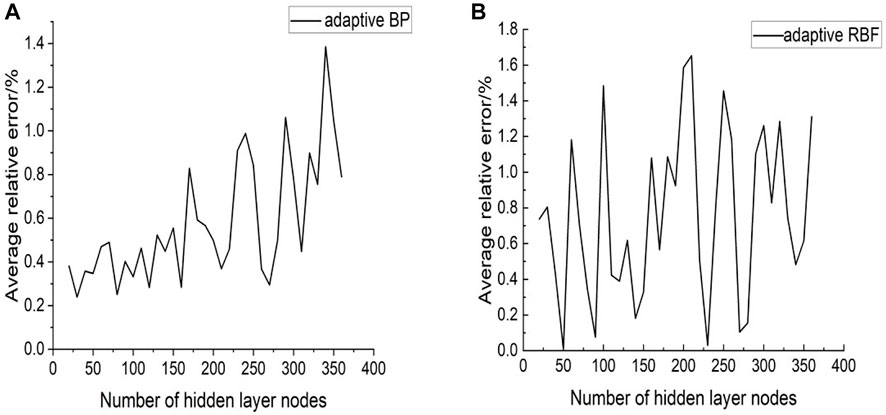
FIGURE 6. Number of hidden layer nodes-average relative error (A) adaptive BP, (B) adaptive RBF.

Figure 6 reveal that within the set number of nodes, the relative error of adaptive BP tends to increase as the number of nodes increases; the minimum number of nodes is 30. The change trend of the mean relative error of the adaptive RBF with the number of nodes is not obvious. Considering that the increase in the number of nodes will increase the amount of calculations, hidden layer nodes are selected to be 40.

3.1.3 Result and analysis

The adaptive BP neural network and the adaptive RBF neural network were used to repeat the experiment 10 times with the same datasets, and the mean values associated with the forecasting results of the test set were determined (Table 2).

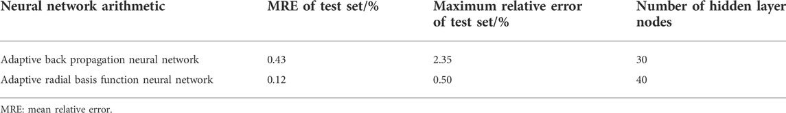
TABLE 2. Comparison of neural network forecast error.

MRE can reflect the degree of dispersion of data samples. The smaller the MRE, the higher the forecast accuracy. Maximum relative error can reflect the degree of maximum deviation from the actual value as well as the fitting ability of local data. By comparing the maximum relative error and MRE of the test sets of the two neural network arithmetics, it is determined that the MREs of both the test sets are less than 1%. A high forecasting accuracy implies that the maximum surface temperature of the fuel rod sheath can be better predicted. The MRE of the adaptive RBF neural network (less than 1%) is extremely similar to the MRE of the test set, indicating that the network has a good fitting effect for local points.

From the above results, it can be summarized that compared to the adaptive BP neural network arithmetic, the adaptive RBF neural network arithmetic exhibits a better forecasting ability for the maximum surface temperature of the fuel rod sheath in the fast reactor core. The reason is that in contrast to the adaptive BP neural network, the adaptive RBF neural network has better generalization capability, can approximate any complex nonlinear function with higher accuracy and obtain high-precision forecasting results for the input data, which shows that it has a good application prospect.

3.2 Transient full reactor analysis

The transient condition is that the coolant flow rate will change significantly with time due to accident working conditions or some reasons, and then other thermal hydraulic parameters of reactors will also change, among which flow instability has a significant impact on reactor safety under transient conditions, so studying the flow instability under the transient conditions is of great significance to the safe operation of reactors. The construction method of neural network under transient conditions is the same as that under steady-state conditions.

3.2.1 Acquisition of data samples

SUBCHANFLOW is used to construct the CEFR 1/2 core model. To reduce the number of calculations, the core sub channel is simplified. It is considered that the axial and radial power density distributions of all the fuel rods in the reactor core area are almost the same; thus, hypothetically combining all coolant channels leads to a bigger channel, whose center is located on the fuel rod with the relevant heating and wetting circumferences (Hu. 2019). For studying the forecasting performance of the neural network under flow instability, the flow change input into the CEFR 1/2 core model is set (Figure 7). This dataset comprises a sine signal and Gaussian white noise signal. Subsequently, the maximum temperature variation in the core fuel sheath is calculated (Figure 8).

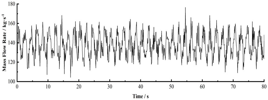
FIGURE 7. Variation in the core inlet flow.

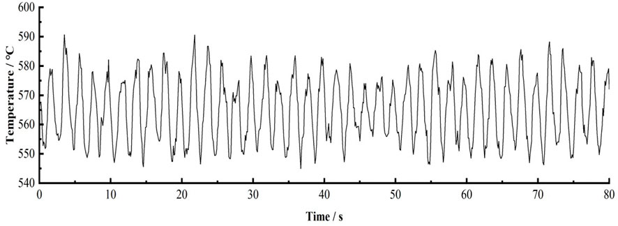
FIGURE 8. Variation in the maximum surface temperature of the fuel rod sheath.

Compared with the steady-state forecasting, the calculation and processing of sample data of transient forecasting will be more complex. To facilitate forecasting, the phase space reconstruction of the flow time series $f\left(i\right)$ and maximum temperature-time series of the sheath t(i) is carried out:

The embedding dimension m is 30, and the time delay $\tau$ is 0.1. A total of 771 datasets were acquired by using the reconstructed core inlet flow vector $F\left(i\right)$ and highest shell temperature vector $T\left(i\right)$ as the input layer, and $F\left(i+\mathrm{m}\tau \right)$ and $T\left(i+\mathrm{m}\tau \right)$ as the output layer. The selection of each data set is consistent with the steady-state conditions. In the adaptive BP neural network, the number of training samples, verification samples, and test samples is 541, 115, and 115, respectively. In the adaptive RBF neural network, the number of training samples and test samples is 617 and 154, respectively. First of all, the neural network for forecasting mass flow rate is trained by Eq. (13), with the neural network input data on the left of the equal sign and the predictive data on the right, and then single-step and continuous forecasting are carried out on the test samples (the next input vectors are replaced by the existing forecasting results).

3.2 2 Analysis of results

The adaptive RBF neural network was used for single-step and continuous forecasting, and the forecasting results were compared with the test values. Figures 9, 10 show that when single-step forecasting is performed, the forecasting accuracy of the reactor core inlet flow is not as good as that of the maximum surface temperature of fuel sheath due to its large noise. The changes in the reactor core inlet flow can still be well controlled; however, in continuous forecasting, since the predictive value will be used as the input value for the next forecast, the error generated by each forecast will affect the next forecast. The predictive value of the core inlet flow is in perfect accordance with the measured value in the first 10 s (Figure 10). In the last 7 s, due to the accumulation of errors, there is a large offset between the predicted value and the measured value, as depicted by the peaks and troughs of the flow oscillation. The accuracy of long-term continuous forecasting is generally low; however, for a short term, the forecasting accuracy of the core inlet flow is higher.

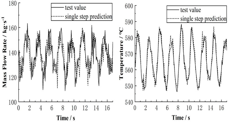
FIGURE 9. Contrast between the test samples and single-step forecasting results.

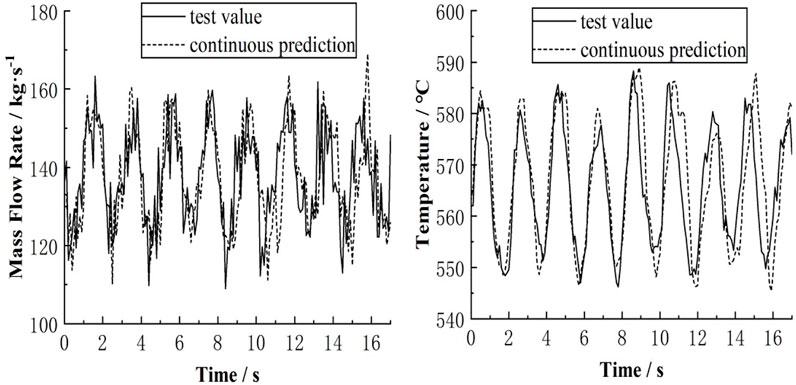
FIGURE 10. Contrast between the test samples and continuous forecasting results.

In singe-step forecasting of the maximum surface temperature of fuel rod sheath, the predictive value is basically the same as the test value; thus, the forecasting accuracy is high. At 7 s, the forecast of the inlet flow of the core suffers a large deviation, leading to a poor forecasting accuracy is poor.

The above results show that for ensuring the accuracy of adaptive neural network prediction results, the time step associated with continuous forecasting needs to be limited. Short-term continuous forecasting performed using the adaptive RBF neural network can accurately forecast the maximum surface temperature of the fuel rod sheath.

Single-step forecasting and continuous forecasting were performed using the adaptive BP neural network and the adaptive RBF neural network, and the forecasting results are listed in Table 3. Table 3 reveals that irrespective of using the adaptive BP neural network or adaptive RBF neural network, the error associated with single-step forecasts is smaller than that of continuous forecasts; however, for the core inlet flow, due to the noise produced by the adaptive RBF neural network, the MREs of single-step forecasting and continuous forecasting are high; there is little difference between the forecasts. The single-step forecasting error for the highest surface temperature of the fuel rod sheath is significantly smaller than the corresponding continuous forecasting error. Comparing the forecasting accuracy of the adaptive BP neural network and the adaptive RBF neural network, it is revealed that for forecasting the reactor core inlet flow and the maximum temperature of the fuel rod sheath, the adaptive RBF neural networks are superior to the adaptive BP neural networks; further, the MREs of single-step forecasting and continuous forecasting are less than those associated with the BP neural networks.

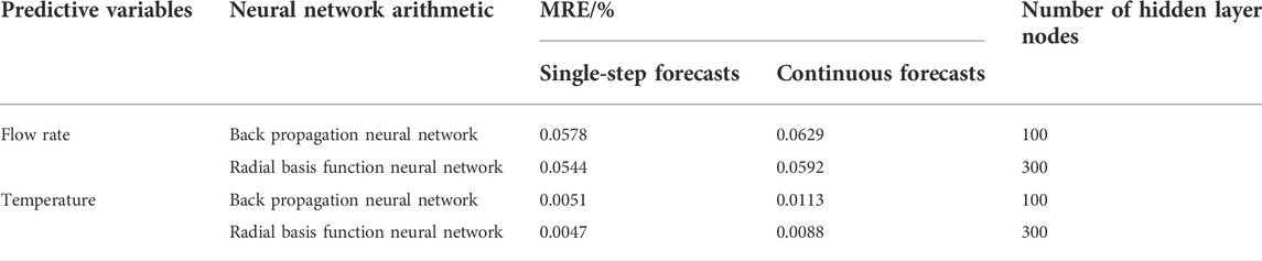
TABLE 3. Comparison of neural network forecasting results.

4 Conclusion

This study aimed to forecast the maximum surface temperature of the fuel rod sheath and the mass flow rate of CEFR under different working conditions. Consequently, different neural network arithmetics are analyzed and compared, and a forecasting method is established for steady-state and transient-state thermal hydraulic parameters of the adaptive RBF neural network model. The main conclusions are as follows:

1) By selecting the 1/2 core model of the CEFR fuel assembly as the research target, forecasting and analysis of the maximum surface temperature of fuel rod sheath under steady-state conditions were performed under the same core background values; the results were repeatedly verified. The results show that the forecasting accuracy of the adaptive RBF neural network is higher than that of the adaptive BP neural network, and its maximum error is 0.5%. Consequently, the adaptive RBF neural network arithmetic has a good application prospect for accurately forecasting the thermal hydraulic parameters of reactors under steady-state conditions.

2) Regardless of single-step or continuous forecasting, the adaptive RBF neural network exhibits a better forecasting accuracy than that of the adaptive BP neural network; however, due to the noise produced by the adaptive RBF neural network, forecasting for certain local points is poor. Nevertheless, the overall forecasting accuracy is good; the MRE associated with forecasting the maximum surface temperature of the fuel rod sheath is no more than 1%, and the MRE of the flow is no more than 6.5%. Therefore, the adaptive RBF neural network can provide reasonably accurate short-term forecasting results and maintain the accuracy under unstable flow conditions, which indicates that it has a good application prospect for real-time forecasting of reactor transients.

3) The adaptive RBF neural network can only complete continuous forecasting in a short time. In the forecasting of transient working conditions, the continuous forecasting error in a short time is acceptable, but with the increase of time, which will become larger because the continuous forecasting error is the superposition of multiple single-step forecasting errors. To solve this problem, further research is needed to improve the single-step forecasting accuracy of neural network; when studying the forecasting performance of the neural network under unstable flow conditions, we used the boundary condition of mass flow rate composed of a sine signal and Gaussian white noise signal. In that case, the transient forecasting accuracy of the adaptive RBF neural network is very good, but there are a large number of transient conditions in the reactor core. In order to further study the adaptability of the method for forecasting key thermal hydraulic parameters under transient conditions, it is necessary to carry out targeted research on different and more complicated boundary conditions.

Data availability statement

The original contributions presented in the study are included in the article/Supplementary Material, further inquiries can be directed to the corresponding author.

Author contributions

JY: analyze the results, writing-original draft preparation. NJ: design the program. PZ: supervision. HW: reviewing and editing.

Funding

This work is supported by the ‘‘Coupled Response Mechanism of Lead-based Fast Reactor Hot Pool and Cold Pool Thermal stratification under Asymmetric Thermal Load Condition and its Influence on Natural Circulation Performance” project of National Natural Science Foundation of China (Grant Nos. 11905101).

Acknowledgments

Thanks are due to all the reviewers who participated in the review and to MJEditor (www.mjeditor.com) for providing English editing services during the preparation of this manuscript.

Conflict of interest

The authors declare that the research was conducted in the absence of any commercial or financial relationships that could be construed as a potential conflict of interest.

Publisher’s note

All claims expressed in this article are solely those of the authors and do not necessarily represent those of their affiliated organizations, or those of the publisher, the editors and the reviewers. Any product that may be evaluated in this article, or claim that may be made by its manufacturer, is not guaranteed or endorsed by the publisher.

References

Azghadi, S., Bonyadi, M. R., and Shahhosseini, H. (2007). Gender classification based on FeedForward backpropagation neural network[J]. Ifip Int. Fed. Inf. Process. 96 (2), 299–304. doi:10.1007/978-0-387-74161-1_32 |
Gomez, A., Jger, W., and Sánchez, V. (2012). “On the influence of shape factors for CHF forecasts with SUBCHANFLOW during a rod ejection transient[C],” in International Topical Meeting on Nuclear Thermal-Hydraulics, Operation and Safety (NUTHOS-9), Taichung, Taiwan, September 4–9, 2022.
Hong, C., Huang, J., Guan, Y., and Ma, X. (2021). Combustion control of power station boiler by coupling BP/RBF neural network and fuzzy rules[J]. J. Eng. Therm. Energy Power 36 (4), 142–148. doi:10.16146/j.cnki.rndlgc.2021.04.021 |
Hu, P. (2019). Study on multi-scale thermal-hydraulic coupling calculation method for reactor core[D]. Harbin: Harbin Engineering University.
Huang, Y., Shan, J., Chen, B., Zhu, J., Lang, X., Jia, D., et al. (2003). Application of artificial neural networks in analysis of CHF experimental data in tubes[J]. Chin. J. Nucl. Sci. Eng. 23 (1), 45–51. doi:10.3321/j.issn:0258-0918.2003.01.008 |
Li, Hui, Wang, Ruipian, and Hu, Shouyin (2003). Application of artificial neural networks in fault diagnosis for 10MW high-temperature das-cooled reactor[J]. Nucl. Power Eng. 24 (6), 563–567. doi:10.3969/j.issn.0258-0926.2003.06.016 |
Li, Wulin, and He, Yujie (2006). The relationship between the number of hidden nodes and the computational complexity of BP network[J]. J. Chengdu Inst. Inf. Eng. (01), 70–73.
Liang, Xi, and Wang, Ruidong (2021). Optimization arithmetic of neural network structure based on adaptive genetic arithmetic[J]. J. Harbin Univ. Sci. Technol. 26 (1), 39–44. doi:10.15938/j.jhust.2021.01.006 |
Lou, jungang, Jiang, yunliang, Shen, qing, and Jiang, jianhui (2013). Evaluating the prediction performance of different kernal functions in kernel based software reliability models. Chin. J. Comput. 36 (06), 1303–1311. doi:10.3724/SP.J.1016.2013.01303 |
Lyu, Y., Zhou, Q. W., Li, Y. F., and Li, W. D. (2021). A predictive maintenance system for multi-granularity faults based on AdaBelief-BP neural network and fuzzy decision making. Adv. Eng. Inf. 49, 101318. doi:10.1016/j.aei.2021.101318 |
Maruyama, M., and Girosi, F., (1992). A connection between GRBF and MLP[J]. Boston, MA: laboratory massachusetts institute of technology.
Mohamedi, Brahim, Hanini, Salah, Ararem, Abdelrahmane, and Mellel, Nacim (2015). Simulation of nucleate boiling under ANSYS-FLUENT code by using RPI model coupling with artificial neural networks[J]. Nucl. Sci. Tech. 26 (04), 97–103. doi:10.13538/j.1001-8042/nst.26.040601 |
Peng, X., Ying, D., Qing, L. I., and Wang, K. (2014). Application of regularized radial basis function neural network in core axial power distribution reconstruction[J]. Nucl. Power Eng. 35 (S2), 12–15. doi:10.13832/j.jnpe.2014.S2.0012 |
Wang, D., Yang, H., Wang, D., Chao, L., and Wang, W. (2020). Research on adaptive BP neural network forecast method for thermal parameters of China experimental fast reactor[J]. Atomic Energy Sci. Technol. 54 (10), 1809–1816. doi:10.7538/yzk.2019.youxian.0751 |
Keywords: radial basis function neural network arithmetic, adaptive gradient descent, fast reactor, thermal hydraulic parameters, forecasting
Citation: Yi J, Ji N, Zhao P and Wu H (2022) Research on the method of predicting CEFR core thermal hydraulic parameters based on adaptive radial basis function neural network. Front. Energy Res. 10:961901. doi: 10.3389/fenrg.2022.961901
Received: 05 June 2022; Accepted: 30 August 2022;
Published: 16 September 2022.
Edited by:
Shripad T. Revankar, Purdue University, United StatesReviewed by:
Xiang Chai, Shanghai Jiao Tong University, ChinaTengfei Zhang, Shanghai Jiao Tong University, China
Copyright © 2022 Yi, Ji, Zhao and Wu. This is an open-access article distributed under the terms of the Creative Commons Attribution License (CC BY). The use, distribution or reproduction in other forums is permitted, provided the original author(s) and the copyright owner(s) are credited and that the original publication in this journal is cited, in accordance with accepted academic practice. No use, distribution or reproduction is permitted which does not comply with these terms.
*Correspondence: Pengcheng Zhao, zpc1030@mail.ustc.edu.cn