A Reconstruction Method for Missing Data in Power System Measurement Based on LSGAN

Introduction

As the power grid-scale continues to grow, especially with renewable energy generation's accession, the power system operation's uncertainty has increased dramatically. The above situation brings unprecedented challenges to ensure the power system’s security and economic operation (Li et al., 2019). In recent years, with the flourishing development of supervisory control and data acquisition systems, as well as the increasing maturity of technologies such as big data and deep learning, power security situation prediction has gradually formed new security warning modes based on data-driven to grasp, control and predict the operation status of the power system, which is different from the traditional modeling and presupposing working conditions. It shows the significant value of data for secure power system operation.

The reliability of measurement data directly affects the conclusions from the data-based analysis of the power system operation behavior. Only conclusions based on reliable data analysis can reflect the system operation's true status (Wang et al., 2020). However, in practice, the supervisory and data acquisition system, due to the data acquisition process, measurement process, transmission modes, storage modes, and other segments, may break down or suffer interference, which will lead to lost or missing data (Jing et al., 2018). To grasp, control, and predict the power system's operation status based on data-driven, the primary problem we need to solve is reconstructing the missing data.

State estimation, a fundamental technology for advanced applications in energy management systems, has made a remarkable contribution to grid data estimation (Ho et al., 2020). On the premise that there are a few missing data and the system has complete observability, we can treat the missing data as data to be estimated and then apply state estimation to estimate the missing data's concrete values (Miranda et al., 2012). Nevertheless, applying state estimation has two major prerequisites: the system needs to meet complete observability, full parameter information (network topology and line parameters). In general, to meet the system’s complete observability, the measurement system provides many redundant data. In the case of a high rate of missing data, the state estimation cannot accomplish the task of estimating missing data when the system's complete observability requirement cannot be satisfied.

Traditionally, the methods for reconstructing missing data are mainly based on the filling method, which can be subdivided into the data filling method based on statistical analysis and the data filling method based on machine learning from the methodological perspective. The former is more common, such as regression Imputation, mean Imputation, and hot-deck Imputation are widely used in practice. The principle is to give reasonable reconstruction values through statistical analysis to reduce the calculation bias caused by missing data (Kallin Westin, 2004). The latter mostly uses supervised learning, semi-supervized learning, and unsupervized learning to achieve the effective reconstruction of missing values (Comerford et al., 2015; Sun et al., 2018; Li et al., 2020). Data reconstruction methods based on statistical analysis are simple and efficient, but reconstructed data accuracy is weak. Although the data reconstruction method based on machine learning class has high accuracy, it requires corresponding multiple mechanism modeling when dealing with multiple missing data, and its practicality is doubtful in the case of high latitude and high missing rate.

The correlations, data distribution characteristics, and data change patterns existing among the power system measurement data can be used as an auxiliary basis for reconstructing the missing data, which can greatly enrich the data's information. The defect of traditional methods is that they do not rationalize the application of such information. The birth of GAN (Generative Adversarial Network) has solved this problem. Initially, GAN made breakthroughs in image inpainting and high-resolution graphic reconstruction (Wang et al., 2017). Indeed, restoring the missing part of the image and reconstructing the missing data of power system measurements belong to the same problem. Both of them generate the missing part following the objective law considering the assigned partial constraints (Dong et al., 2019). In the image restoration problem, GAN can automatically learn the complex distribution pattern among data through the training of neural network in an unsupervized form, and then generate the data to meet the objective law, solving the problem of high data latitude and complex modeling (Wu et al., 2017).

GAN has attracted scholars from home and abroad, and many studies have been conducted. J. Lan et al. have proposed a CGAN (Conditional Generative Adversarial Networks) model with the inclusion of classification label information to enrich the original true and false binary classification into a multi-type determination. The introduced label information can be used as an additional criterion to verify the generation results and contribute to the correction of the generation results (Lan et al., 2018). A. Borgia et al. have applied GAN to generate pedestrian walking postures and Interpolate the video to enrich the video information, thus improve the accuracy of pedestrian recognition (Borgia et al., 2019). C. Ledig et al. proposed the SRGAN (Super-Resolution Generative Adversarial Networks) model to accomplish the task of improving the image resolution (Ledig et al., 2017). In the domain of missing image restoration, M. Wang et al. applied GAN to reconstruct the obscured part of the face in the image to enrich the training sample, thus improving the accuracy of recognizing facial expressions (Wang et al., 2019a). R. A. Yeh et al. applied a deep generative model to the image reconstruction problem to guarantee that the image realism constraint is satisfied during reconstruction (Yeh et al., 2017). To solve the problem of gradient disappearance and dispersion during GAN training, S. Wang et al. replaced the original objective function to train GAN with minimized Wasserstein distance as the objective function, which improved the stability of training. However, applying WGAN makes computational efficiency significantly decreased (Wang et al., 2019b).

In summary, data restoration methods based on statistical analysis are relatively simple and straightforward but not very practical in the case of high dimensionality and high loss rates. The state-estimation-based data restoration method is limited by the conditions required for mechanism modeling, and the available premise is that absolute preconditions must be provided. The GAN-based data restoration method solves the former deficiency to some extent. It overcomes the limitations of conditions for the method and can still reconstruct data and restore data in high-dimensional and high-lost rate cases. However, the original GAN may suffer from gradient disappearance and dispersion during training due to the loss function's limitation. The improved WGAN, a GAN derivative method, solves gradient disappearance during training by modifying the loss function. Nevertheless, the consequent computational burden makes the training efficiency drop significantly. It is worth investigating how to find a generative adversarial network that can overcome the gradient disappearance and consider computational efficiency.

In this paper, we propose to apply LSGAN (Least Squares Generative Adversarial Networks) to the problem of reconstructing missing data from power system measurements. The proposed method learns the data's objective distribution pattern to generate highly accurate reconstructed data that conforms to the inter-data complex pattern. Unlike other GANs, LSGAN replaces the cross-entropy loss function with the least-squares loss function when applying GAN in reconstructing missing data. We use this different distance metric from the traditional one to build an adversarial network with more stable training, faster computational convergence, and higher quality in the generated data. It solves unstable training due to gradient disappearance and diffusion and the low computational efficiency of traditional GANs. The experimental results show that comparing with GAN, CGAN, and WGAN methods, the data generated by LSGAN can still guarantee high accuracy in the case of multiple data missing, which provides a good data basis for applying large volume data to analyze the power system operation behavior.

Related Work

Generating Adversarial Networks

GAN is an unsupervized learning model. It was first proposed by Ian J. Goodfellow and other researchers in 2014 (Goodfellow et al., 2014a). GAN was mainly used to generate images in unsupervized training mode in the beginning. It shows the effect of generating handwritten digital images by GAN training with the MNIST training dataset as the sample in Figure 1. We can see that evolution from the initial noise-filled image to a cleaned handwritten digital image.

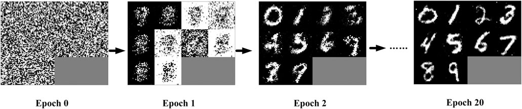
FIGURE 1. The schematic diagram for the effects of GAN in generating images within the iterative training process.

The model embodies the idea of a “zero-sum game”: for the two participants in the game, under tough competition, if one gains, it must mean that the other loses. The sum of gains and losses for both participants is always “zero,” and there is no possibility of cooperation between them. With this concept of the non-cooperative game, GAN is composed of Generator and Discriminator.

Generator is a neural network used to learn the distribution pattern of data within a sample and generate new sample data to meet the pattern accordingly. The technical route: the Generator trains an arbitrarily distributed vector z to obtain $x^{\prime }=G\left(z\right)$, where $x^{\text{'}}$ is obeying distribution $P_G\left(x\right)$. Then we obtain the optimal solution $G^{\ast }$ by modifying the Generator's internal weight parameters to obey the real data distribution $P_{\mathrm{data}}\left(x\right)$. Then there is the following equivalence relation: $P_G\left(x\right)\approx P_{\mathrm{data}}\left(x\right)$. According to the above idea, the expression of $G^{\ast }$ is as shown in Eq. 1:

Discriminator is also a neural network, a binary classifier mainly used to determine whether the input data is from the sample data or the generated data. Its purpose is to discriminate the disparity between the original and generated samples more precisely. The disparity can be expressed in Eq. 2 as follows:

Where ${{\rm E}}_{x\sim P_{\mathrm{data}}}$ denotes the expectation of x within the sample distribution $P_{\mathrm{data}}\left(x\right)$. ${{\rm E}}_{x\sim P_G}$ denotes the expectation of x within the sample distribution $P_G\left(x\right)$.

The Discriminator aims at maximizing $v\left(D,G\right)$. $\underset{D}{\max }v\left(D,G\right)$ makes Discriminator better distinguish between D and G. The larger the value of $\log D\left(x\right)$ and the smaller the value of $\log \left(1-D\left(x\right)\right)$, the trained Discriminator gets higher the discriminative accuracy.

We denote $\underset{D}{\max }v\left(D,G\right)=\text{Div}\left(P_{\mathrm{data}}\left(x\right),P_G\left(x\right)\right)$, then $G^{\ast }=\text{arg}\{\underset{G}{\min }\underset{D}{\max }v\left(D,G\right)\}$. The Discriminator’s goal is to maximize the gap between the generated data distribution and the true data distribution. The Generator's goal is to minimize the gap between the generated data distribution and the true data distribution.

In summary, the Discriminator in GAN is trained to maximize the correctness of the labels assigned to the sample data and the “generated data.” The Generator in GAN is trained to minimize the correct recognition of the “generated data” by the Discriminator. This adversary training process allows the Discriminator to reach the Nash equilibrium. Meanwhile, the Generator can generate “generated data” similar to the sample data and successfully “trick” the Discriminator.

According to the proof procedure in the companion paper, we can see that Eq. 3 is the minimized Jensen-Shannon divergence (Goodfellow et al., 2014a):

The original GAN has one defect: initially, the distribution of the “generated data” obtained by the Generator may not overlap with the real data distribution. In this case, using the original JS divergence as a measure of the “distance” between the two distributions may fail. It results in the gradients disappearing and diffusing during training, thus failing to generate high-quality data.

Conditional Generative Adversarial Networks

CGAN is a conditional generative adversarial networks model based on the GAN with conditional extensions. Suppose both the Generator and the Discriminator apply to some additional condition y, such as class labels. In that case, the data can be calibrated during the generation process by attaching y to the input layer for input to the Generator and Discriminator.

In the Generator, the noise is input along with the corresponding condition y, and the real data x and condition y are used as the Discriminator's objective function. According to the corresponding literature's derivation process, we can obtain Eq. 4 (Mirza and Osindero, 2014).

From the above equation, the optimization process of CGAN for the objective function $v\left(D,G\right)$ is similar to that of GAN. Where ${{\rm E}}_{x\sim P_{\mathrm{data}}}\log D\left(x|y\right)$ denotes the probability that the Discriminator identifies whether the data x is real data under condition y; ${{\rm E}}_{x\sim P_G}\log \left(1-D\left(x|y\right)\right)$ denotes the probability that the generated data x is judged to be real data by the Discriminator under condition y.

In summary, it can be seen that CGAN is an improvement of the unsupervized GAN model into a supervised model. The added condition helps to improve the accuracy of the generated data. However, since the objective function continues to use the GAN’s objective function, there remains a scenario when the data distribution pattern of generated data $P_G$ differs significantly from that of data $P_{\mathrm{data}}$. It can make the case that the Generator’s generated data would never pass the Discriminator’s validation, and thus the gradient disappears and diffuses.

Wasserstein Distance-Based Generative Adversarial Networks

Both the original GAN and CGAN have the same problem: applying JS divergence as a measure of the “distance” between two distributions leads to the gradients disappearing and dispersion in training. In response to these problems, WGAN uses the Wasserstein distance to measure the difference between the true data distribution and the generated data distribution (Arjovsky et al., 2017).

The Wasserstein distance, also called Earth-Mover distance, is used to measure the distance between two distributions. Its expression is shown in Eq. 5:

Where $\Pi \left(p_d,p_g\right)$ is the set of all joint distributions after the combination of p_d and p_g. ${{\rm E}}_{\left(x,y\right)\sim \lambda }\Vert x-y\Vert$ is the expected value of the distance between the true sample x and the generated sample y under compliance with the joint distribution λ. $\underset{\lambda \sim \prod \left(p_d,p_g\right)}{\inf }{{\rm E}}_{\left(x,y\right)\sim \lambda }\Vert x-y\Vert$ is the lower bound that we manage to take for this expected value among all possible joint distributions.

For this Earth-Mover distance, we can intuitively interpret it as the “distance” used to move the “mound (p_d)” to the location of the “mound (p_g)” under the “planning path” of λ. $W\left(p_d,p_g\right)$ is the minimum distance under the “optimal path.”

Wasserstein's advantage over traditional distance measures is that Wasserstein distance can still describe the distance between two distributions even if they do not overlap, overcoming the problem of gradient disappearance and dispersion in training due to no overlap between the two distributions. Although WGAN solves gradient disappearance and dispersion in training, the additional computational load increases the computational cost and reduces the training efficiency.

Least Squares Generative Adversarial Networks

LSGAN is an optimization model of GAN proposed by Mao Xudong and other scholars in 2017 (Mao et al., 2017). It mainly addresses the traditional GAN’s two defects: the low quality of the generated images and the training process's instability. The difference is that GAN’s objective function is changed from the cross-entropy loss function to the least-squares loss function. Consequently, a more stable and faster converging adversarial network with high generation quality is born.

The objective function of LSGAN is defined as Eq. 6 (Mao et al., 2017).

Where a and b denote the labels of the fake and true data, respectively. c denotes the value that the Generator expects the Discriminator to trust for the fake data (Ma et al., 2019).

Two options are given for the values of a, b, c.

1) Add $\left(1/2\right){{\rm E}}_{x\sim p_{\mathrm{data}}\left(x\right)}{\left(D\left(x\right)-c\right)}^2$ to Eq. 6. Since $\underset{G}{\min }{V}_{LSGAN}\left(G\right)$ does not contain the generator parameters, it does not change the optimal solution. Thus we can obtain Eq. 7.

Maintaining the Generator constant, we can obtain the optimal solution of the Discriminator as in Eq. 8.

From Eqs. 7, 8, we derive Eq. 9.

If we set b-c = 1 and b-a = 2, we can obtain the following equations.

where ${\chi }_{\mathrm{Pearson}}^2$ is the Pearson chi-square divergence. For example, when we set a = -1, b = 1, and c = 0, the objective function is as follows:

2) By setting b = c, the Generator generates data that is as similar as possible to the true data distribution. For example, if we set a = 0 and b = c = 1, respectively, the objective function is as follows:

The main idea of LSGAN is to provide a smoothing and non-saturating gradient loss function for the Discriminator. In this way, D “pulls” the data generated by the generator G to the true data distribution P_data (x), so that the distribution of the data generated by G is similar to P_data (x). In this paper, we choose the second scheme as the objective function.

LSGAN-Based Method for Reconstructing Missing Power Data

Data does not exist in isolation. There are often various constraints between data, which describe the relationship between the data. The data must meet this correlation between the data and not be contradicted by each other. There is a constraint relationship between the power data in the power system: during the system's operation, the power balance is satisfied at all times.

The power grid is composed of nodes and lines. The grid's power balance can be divided into two types of balance: node power balance and line power balance. For the node, the power directly related to the node satisfies the principle that the total power injected into the node is equal to the total power out of the node. For the line, the difference of the actual power at both ends is the power loss of branches.

The blue blocks in Figure 2 represent normal power data, and the red blocks represent missing power data.

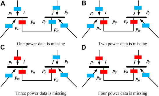
FIGURE 2. Schematic diagram of the missing active power data in different cases.

When the case in a) occurs, P_ij power data is missing. According to the line power balance principle, we can reconstruct the missing data Pij by the power at the other end of the branch, and the branch loss power. We can also reconstruct the missing power P_ij by directly related to node i according to the node power balance principle.

When the case in b) occurs, P_ij and P_ji power data are missing. We can reconstruct the missing power P_ij and P_ji by directly correlating the power with node i and node j, respectively, according to the node power balance principle.

When the case in c) occurs, the missing power P_ji can be reconstructed according to the node power balance principle by directly correlating the power with node j. Then the missing power P_ij according to the line power balance principle. Finally, the missing power P_ii can be reconstructed according to the node power balance principle by directly correlating the power with node i.

When the case in d) occurs, the system does not meet the observability. We can no longer complete the data reconstruction task by applying the power balance principle alone. The data reconstruction method in this paper can solve this problem.

The data we currently acquire are fully structured data recorded at the same time sampling scale with the correlation measurements of different stations. There are topological linkage relationships between the physical objects it represents, so each time section’s data are data with topological constraints.

Unlike regular data, power system measurement data embody spatially constrained relationships between each other. Therefore, we can add spatiality to the characteristics of describing data. By organically integrating the grid data's spatial correlations with the grid power data, we can enrich the data’s distribution characteristics and enhance the data’s representable dimensions. It contributes to improving the learning effect of generative adversarial networks on data characters.

We use the adjacency matrix A to describe the network topology. If a topology consists of n nodes, its adjacency matrix is an n × n matrix $A\in {ℝ}^{n\times n}$. The values of each element a_ij inside it are as follows:

Where v is a one-dimensional array storing information about the graph's vertices, v_i and v_j denote node i and node j. E is a two-dimensional array storing information about the edges (nodes directly interconnected) in the graph. $\left(v_i,v_j\right)\in E$ means that node i and node j are directly interconnected. Otherwise, the two nodes are not directly connected.

We place the adjacency matrix’s non-zero elements to the line active power P_ij and place the diagonal elements to the node injected active power value P_ii. The node active power correlation matrix P_relation is thus generated as shown in Eq. 14, $P_{\mathrm{relation}}\in {ℝ}^{n\times n}$.

The node active power correlation matrix P_relation forms the database for describing the grayscale map of active power distribution in a single section. The magnitude of the matrix’s values determines the corresponding color blocks' lightness and darkness in the grayscale map. We can analogize the process of generating new pictures by unsupervized learning in generative adversarial networks to reconstruct the missing power data. The specific process is shown in Figure 3.

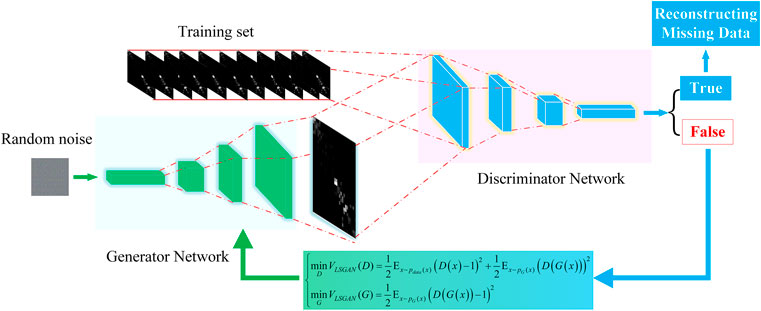
FIGURE 3. Flow chart of the reconstruction method for missing power data based on LSGAN.

Experiment and Results

Experimental Results on a Test Sample

In this paper, the IEEE14-bus system shown in Figure 4 was used to verify the proposed method’s effectiveness. The network consisted of 14 nodes and 20 equivalent transmission lines. To make the examples more general, we increased each load in the example system by 1–10% in equal proportions, for a total of 10 growth percentages, while not changing the rated output of the generator nodes. A Gaussian perturbation of 0.01 was added to each growth amount to generate 1,000 data samples for 10,000 data samples.

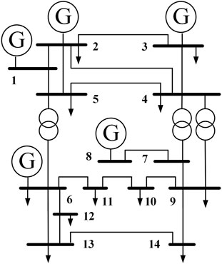
FIGURE 4. IEEE14-bus system network topology.

The nodal active power correlation matrix P_relation and the nodal reactive power correlation matrix Q_relation were generated for these data samples according to the nodal active power correlation matrix’s composition mode. We stitched the two matrices together along the diagonal to form a new matrix Y, $Y\in {ℝ}^{n\times n}$:

We set the base values of active and reactive power as P_base = 500 MW and Q_base = 50 MW and then took the standardized values for the Y matrix's active and reactive parts, respectively. Thus, the normalized power correlation matrix X was generated.

If we mapped the normalized power correlation matrix X as a graph, then the magnitude of the matrix X values determined the color block's lightness or darkness at the corresponding position. The original sample data mapping graph is shown in Figure 5.

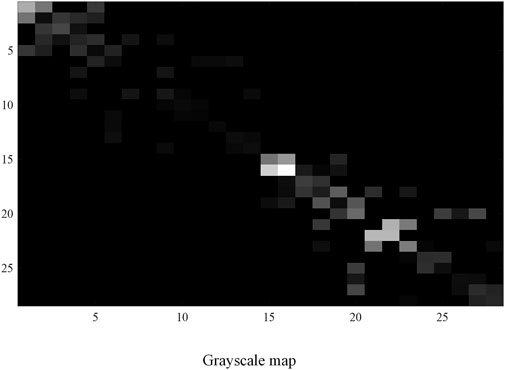
FIGURE 5. The grayscale map is drawn from the original sample data.

As seen in Figure 5, the data distribution characteristics shown in the graph are that the data are concentrated around the diagonal, and the upper and lower triangles are approximately symmetric. It is consistent with the distribution characteristics of the original data.

We divided the above 10,000 data samples into the training set and test set in the ratio of 8:2. The dimension of the training set X_train was (28,28,8000), and the dimension of the test set X_test was (28,28,2000). On the test set X_test, we set 10 active power missing and 10 reactive power missing in their node power correlation matrix. The specific information was node injected power: P_1-1, P_3-3, Q_1-1, Q_2-2, Q_6-6, Q_8-8, and line power: P_1-2, P_2-1, P_5-1, P_3-2, P_5-2, P_2-3, P_5-4, P_4-5, Q_1-2, Q_2-1, Q_4-5, Q_5-4, Q_8-7, Q_7-8.

We set the batch training number of GAN, CGAN, WGAN, and LSGAN to 32 and the maximum number of training epochs to 50. Regarding the optimizer, we chose to use Adaptive Moment Estimation (Adam). Based on the comparison of the relevant parameters in the literature (Ruder, 2016), we set the parameters as follows: Image size was 28 × 28, the learning rate of the Discriminator was 3e-4, the learning rate of the Generator was 3e-4, beta1 was 0.5, and beta2 was 0.999.

We got the mapping graphs of the data generated under the same training batch at each method’s 50th epoch. Then they were used to compare and analyzed the effectiveness of learning data features by each method. The results were shown in Figure 6.

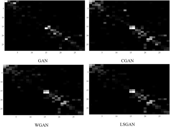
FIGURE 6. The grayscale map is drawn from the generated data by GAN, CGAN, WGAN, LSGAN.

As can be seen from Figure 6, the data generated by each method display the main distribution characteristics of “the data are concentrated around the diagonal, and the upper and lower triangles show approximate symmetry.” However, judging from the details, the grayscale map of the data generated by LSGAN is most close to the grayscale map of the original sample. The data generated by GAN differs significantly from the original data. Both CGAN and WGAN methods are deficient in the accuracy of generating non-diagonal data.

To further measure the accuracy of the data generated by the above four methods, we counted the absolute error (AE), absolute percentage error (APE) of the 20 sets of missing data corresponding to the generated data under the 50th epoch of each method. The mean and standard deviation statistics were shown in Tables 1, 2.

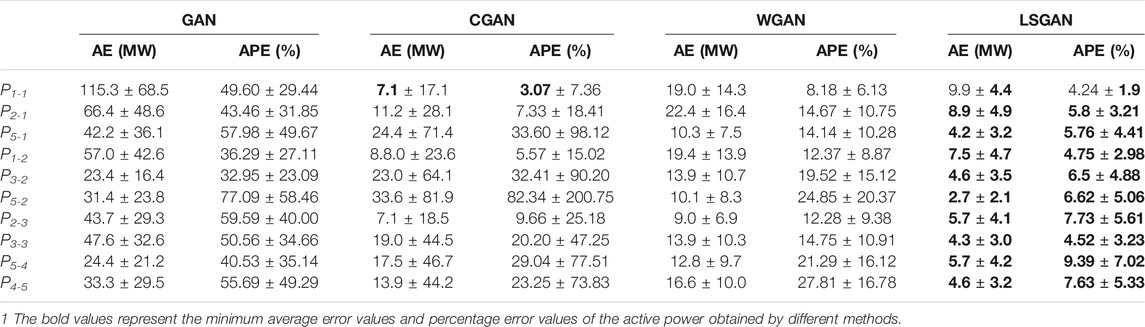
TABLE 1. The AE and APE statistics of the generated active data.

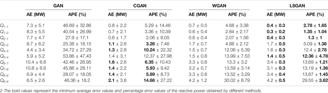
TABLE 2. The AE and APE statistics of the generated reactive data.

As seen in Tables 1, 2, the LSGAN method generates data with small errors and the highest accuracy in most of these cases. Although the error of the generated data under the CGAN method in some measurements is smaller than the error of the generated data based on the LSGAN method, the LSGAN method is more stable in terms of standard deviation. These indicate that LSGAN outperforms the other three methods in most cases in terms of generating data effects.

To obtain the training effect of the proposed method in the training process, we counted the computation time consumed and the reconstructed data's average accuracy under different epochs. The results were shown in Figures 7, 8.

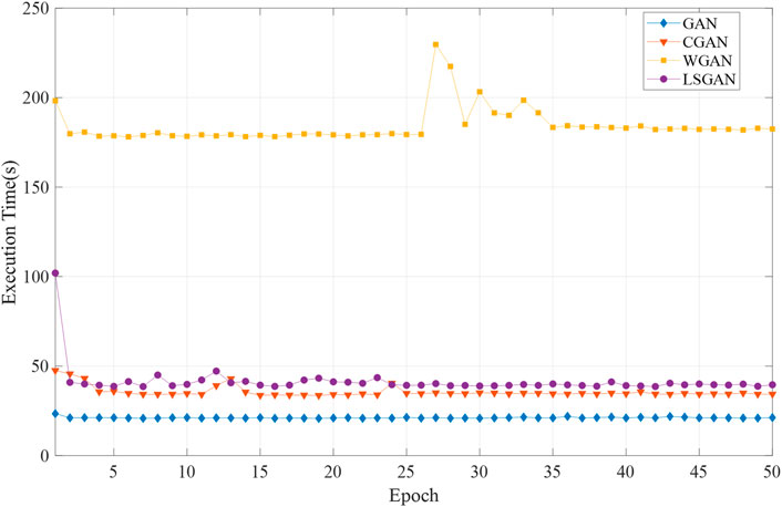
FIGURE 7. Computational time consumption curves for each training cycle of different methods.

FIGURE 8. Mean accuracy of reconstructed data by different methods during the training process.

As seen in Figure 7, GAN is the most efficient in terms of computational efficiency. CGAN and LSGAN are approximately more efficient than WGAN. WGAN takes the most time to compute and is the least efficient.

As seen in Figure 8, the highest accuracy of the data reconstructed by GAN is only 58.19%, and the training effect is unstable. It is mainly due to the gradient disappearance and dispersion during the training process. CGAN makes the accuracy of the reconstructed data reach 90.24% in the first 7 epochs. It indicates that the method can obtain the reconstructed data with high accuracy in a short training period. However, the accuracy of the reconstructed data by CGAN decreases as the training continues. It indicates that although CGAN improves the GAN-based reconstructed data’s accuracy, the training instability still exists. The accuracy of the data reconstructed by WGAN steadily increased during the continuous training process and finally reached 86.13%. In contrast, the accuracy of the data reconstructed by LSGAN is not as high as that of CGAN in a short period. However, the accuracy of the generated data has been steadily improving with increasing training epochs, and the highest accuracy reaches 93.57%, which is significantly better than the other three methods.

Experimental Results on LSGAN

In this section, we applied the IEEE 39-bus system and the IEEE 118-bus system to test the method’s effectiveness in this paper. The IEEE 39-bus system had 39 nodes and 46 lines. The dimension of the nodal active power correlation matrix P_relation-39, which was composed based on this system’s tide data, was 39 × 39. We followed the LSGAN-related parameters in the previous section and modified the weight coefficient matrix dimension to fit the nodal active power correlation matrix derived from the IEEE 39-bus system.

We added a 1% Gaussian perturbation to each load in the test system without changing the generator nodes’ rated output to generate 1,000 data samples as training samples. The proposed method was then trained iteratively for 50 epochs, generating 250 data samples per epoch. We selected some nodes active power and directly associated line power as missing data, as follows: P_1-1, P_2-1, P_1-2, P_3-2, P_2-3, P_3-3, P_4-5, P_5-6, P_4-4, P_5-4

We counted the absolute error (AE), absolute percentage error (APE) of the 10 sets of missing data corresponding to the generated data under each method’s 50th epoch. The mean and standard deviation statistics were shown in Table 3.

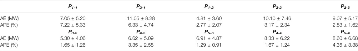
TABLE 3. The AE and APE statistics of the generated reactive data (IEEE 39-bus system).

As seen from the above table, the generated data have few errors, and the majority of the generated data have an accuracy of over 92%. The difference between data-driven and mechanism-based modeling is that the former is not constrained by the system operating conditions. The above process is executed under whole network conditions. How effective the proposed method is under partial data conditions. We performed the following experiments: we extracted bus 1–14 in the whole network to form a cut-set network, and the cut-set network was made to contain all missing measures. We treat the contact line between the cut-set network and the whole network as a separate line. Then we modify the dimensionality of the relevant parameters within LSGAN to fit the new network. The accuracy of the generated data changes under the two network forms is counted. The average accuracy of the generated data trained by the whole network and the cut-set network under different training cycles is compared as shown in Figure 9.

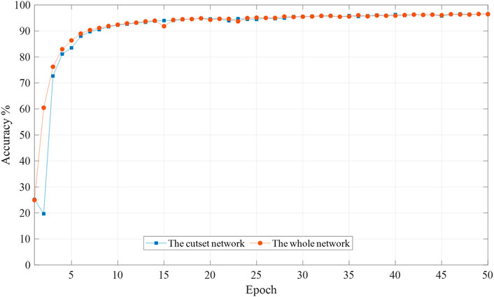
FIGURE 9. Mean accuracy of reconstructed data by different network forms during the training process (IEEE 39-bus system).

As can be seen from the above figure, the data generated by the whole network (39 buses) is more accurate than that generated by the cut-set network (14 buses) at the beginning of the training process. In the later period, the data accuracy of both generated data is the same. The data-driven data restoration approach does not rely on external conditions such as network parameters and does not require complete network data. The purpose of data restoration can also be achieved with cut-set data.

We made similar experiments as above in the IEEE 118-bus system. The IEEE 118-bus system had 118 nodes and 186 lines. The dimension of the nodal active power correlation matrix P_relation-118, which was composed based on this system's tide data, was 118 × 118. We followed the LSGAN-related parameters in the previous section and modify the weight coefficient matrix dimension to fit the nodal active power correlation matrix derived from the IEEE 118-bus system.

We selected some nodes' active power and directly associated line power as missing data, as follows: P_4-5, P_5-8, P_8-9, P_10–9, P_15–15, P_15–17, P_25–23, P_25–25., P_26–26, P_25–27. We counted the absolute error (AE), absolute percentage error (APE) of the 10 sets of missing data corresponding to the generated data under each method's 50th epoch. The mean and standard deviation statistics were shown in Table 4.

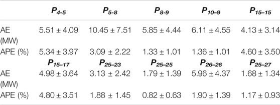
TABLE 4. The AE and APE statistics of the generated reactive data (IEEE 118-bus system).

As seen from the above table, the generated data have minor errors, and the majority of the generated data have accuracy above 95%. It indicates that the method in this paper can be extended to apply in larger networks. To further verify whether the cut-set network still works in large networks, we select a cut-set network consisting of bus 1–30 for training, containing all the missing data. The average accuracy of the generated data trained by the whole network (118 nodes) and the cut-set network (30 nodes) under different training epochs are compared, as shown in Figure 10.

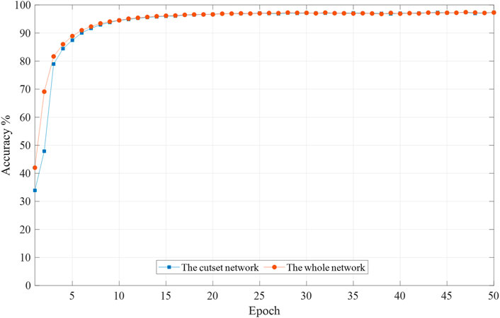
FIGURE 10. Mean accuracy of reconstructed data by different network forms during the training process (IEEE 118-bus system).

As shown from the above figure, the test results are similar to those of the IEEE 39-bus system test. At the beginning of the training process, the accuracy of the data generated by the whole network training is higher than that of the data generated by the cut-set network training. With continuous iterative training, the two generated data with the same accuracy at the later stage. Although the accuracy is similar between the two networks, the cut-set network is used as the training sample to streamline the data’s composition and decrease the non-essential data. The computation time is only 1/10 of the whole network, which greatly improves the computation efficiency.

LSGAN does not depend on external operating conditions' constraints but needs to have sample data as the necessary foundation. With the great development of power system information, the power grid has established many measurement systems reflecting the system operation status, such as the SCADA system, which records active power, reactive power, voltage, and power grid frequency. The sampling interval of this system is 1 min, and each measurement day records 1,440 data. The amount of SCADA data recorded by a provincial power grid in a day can reach several GB, which provides a good training sample base for this paper's method. Grid measurement data has spatial and temporal properties. When there is a high dimensional and high loss rate case in the power grid, the data before and after the time series can be used as training samples to identify the missing data, and the data at the same time every day can be used as supplementary samples to assist in determining the missing data. The actual system is complex and variable. How to construct the internal architecture of LSGAN, select the sample data, and apply this paper to the actual system needs to continue to be studied in-depth, which is not discussed too much in this paper.

Conclusion

This paper’s main contribution is to propose a method based on LSGAN to reconstruct missing data for missing measurement data in power systems. We transformed the problem of reconstructing missing data into the problem of repairing missing parts in images. The method in this paper provided a new approach to solve the problem of restoring missing data. LSGAN learned correlations and distribution features among data by unsupervized self-gaming training mode. By changing the latent parameters in the Generator, it enabled the Generator to generate data that matched the objective laws of real data. The proposed method was able to cope with data loss in power systems due to improper handling and provide a solid technical basis for ensuring data integrity.

Unlike the traditional GAN model, LSGAN replaced the original objective function from cross-entropy loss function to least-squares loss function. It ensured gradient descent by penalizing those samples far from the decision boundary, solving gradient disappearance and dispersion. Moreover, the least-squares iterative computation was efficient.

It was experimentally verified that the proposed method could still reconstruct the missing data in the case of multiple power data missing. In the comparison experiments with GAN, CGAN, and WGAN models, respectively, the LSGAN-based data reconstruction method could steadily improve the generated data accuracy during the continuous training process with higher final accuracy than GAN, CGAN, and WGAN models under the same epoch. The computational efficiency was 4.5 times higher than that of WGAN.

The method in this paper was entirely data-driven and did not involve mechanistic modeling. A cut-set network could be constructed on-demand to streamline the composition of the data, thus avoiding non-essential computational burden, and its accuracy was similar to that of data generated by the overall network training. The method was able to generate data with high accuracy for the restoration data problem. It was mainly because the least squares-based loss function imposes a large penalty on the boundary data. Although it enabled to improve the accuracy of the generated data, the method had some limitations for cases where diverse sample data needed to be generated.

In this paper, the proposed method was validated based on the IEEE 14-bus system, IEEE 39-bus system, and IEEE 118-bus system. The feasibility of the method was demonstrated. It should be noted that many issues are worthy of attention and further study for application to actual large-scale power grids. For example, designing LSAGN internal deep neural networks for large-scale power systems and how to select the training set reasonably are all issues that we plan to study in-depth in the future.

Data Availability Statement

The raw data supporting the conclusions of this article will be made available by the authors, without undue reservation.

Author Contributions

Conception and design of study: CW Acquisition of data: SZ Drafting the manuscript: YC, TL Analysis and interpretation of data: CW, YC Revising the manuscript critically for important intellectual content: YC, CW.

Funding

This work was supported by the National Natural Science Foundation of China (No. 51437003).

Conflict of Interest

The authors declare that the research was conducted in the absence of any commercial or financial relationships that could be construed as a potential conflict of interest.

References

Arjovsky, M., Chintala, S., and Bottou, L. (2017). “Wasserstein generative adversarial networks,” in Proceedings of the 34th international conference on machine learning-volume 70, Sydney, Australia, August 6–11, 2017. Editor D. Precup, and Y. Whye Teh (Sydney, NSW, Australia: JMLR.org), 214–223.
Borgia, A., Hua, Y., Kodirov, E., and Robertson, N. (2019). “GAN-based pose-aware regulation for video-based person Re-identification,” in 2019 IEEE winter conference on applications of computer vision (WACV), Waikoloa Village, HI, January 11, 2019 (New York, NY: IEEE), 1175–1184. doi:10.1109/WACV.2019.00130
Comerford, L., Kougioumtzoglou, I. A., and Beer, M. (2015). An artificial neural network approach for stochastic process power spectrum estimation subject to missing data. Struct. Saf. 52, 150–160. doi:10.1016/j.strusafe.2014.10.001
Dong, J., Yin, R., Sun, X., Li, Q., Yang, Y., and Qin, X. (2019). Inpainting of remote sensing SST images with deep convolutional generative adversarial network. IEEE Geosci. Remote Sensing Lett. 16 (2), 173–177. doi:10.1109/LGRS.2018.2870880
Goodfellow, I. J., Pouget-Abadie, J., Mirza, M., Xu, B., Warde-Farley, D., Ozair, S., et al. (2014a). “Generative adversarial nets,” in Advances in neural information processing systems, Montreal, QC, Demember 8–13, 2014 (CanadaCurran Associates, Inc.).
Ho, C. H., Wu, H. C., Chan, S. C., and Hou, Y. (2020). A robust statistical approach to distributed power system state estimation with bad data. IEEE Trans. Smart Grid 11 (1), 517–527. doi:10.1109/Tsg.2019.2924496
Jing, L., Wei, L., and Sheng, Y. (2018). Research on abnormal diagnosis for power grid equipment archival data based on machine learning. Electric Power Inf. Commun. Tech. 16 (7), 21–27. doi:10.16543/j.2095-641x.electric.power.ict.2018.07.004
Kallin Westin, L. (2004). Missing data and the preprocessing perceptron. Umeå, Sweden: Umeå University.
Lan, J., Guo, Q., and Sun, H. (2018). Demand side data generating based on conditional generative adversarial networks. Energ. Proced. 152, 1188–1193. doi:10.1016/j.egypro.2018.09.157
Ledig, C., Theis, L., Huszár, F., Caballero, J., Cunningham, A., Acosta, A., et al. (2017). “Photo-realistic single image super-resolution using a generative adversarial network,” in 2017 IEEE conference on computer vision and pattern recognition (CVPR), Honolulu, HI, July 21–26, 2017 (New York, NY: IEEE), 105–114. doi:10.1109/CVPR.2017.19
Li, L., Liu, H., Zhou, H., and Zhang, C. (2020). Missing data estimation method for time series data in structure health monitoring systems by probability principal component analysis. Adv. Eng. Softw. 149, 102901. doi:10.1016/j.advengsoft.2020.102901
Li, Y., Yang, Z., Li, G., Zhao, D., and Tian, W. (2019). Optimal scheduling of an isolated microgrid with battery storage considering load and renewable generation uncertainties. IEEE Trans. Ind. Electron. 66 (2), 1565–1575. doi:10.1109/TIE.2018.2840498
Ma, J., Yu, W., Liang, P., Li, C., and Jiang, J. (2019). FusionGAN: a generative adversarial network for infrared and visible image fusion. Inf. Fusion 48, 11–26. doi:10.1016/j.inffus.2018.09.004
Mao, X., Li, Q., Xie, H., Lau, R. Y. K., and Smolley, S. P. (2017). “Least squares generative adversarial networks,” in 2017 IEEE international conference on computer vision (ICCV), Venice, Italy, October 22, 2017 (New York, NY: IEEE), 2813–2821. doi:10.1109/ICCV.2017.304
Miranda, V., Krstulovic, J., Keko, H., Moreira, C., and Pereira, J. (2012). Reconstructing missing data in state estimation with autoencoders. IEEE Trans. Power Syst. 27 (2), 604–611. doi:10.1109/TPWRS.2011.2174810
Mirza, M., and Osindero, S. (2014). Conditional generative adversarial nets. arXiv:https://arxiv.org/abs/1411.1784.
Ruder, S. (2016). An overview of gradient descent optimization algorithms. arXiv:https://arxiv.org/abs/1609.04747.
Sun, Y.-Y., Jia, R.-S., Sun, H.-M., Zhang, X.-L., Peng, Y.-J., and Lu, X.-M. (2018). Reconstruction of seismic data with missing traces based on optimized Poisson Disk sampling and compressed sensing. Comput. Geosci. 117, 32. doi:10.1016/j.cageo.2018.05.005
Wang, C., Mu, G., and Cao, Y. (2020). A method for cleaning power grid operation data based on spatiotemporal correlation constraints. IEEE Access 8, 224741–224749. doi:10.1109/ACCESS.2020.3044051
Wang, K., Gou, C., Duan, Y. J., Yilun, L., and Zheng, X. H. (2017). Generative adversarial networks: the state of the art and beyond. Zidonghua Xuebao/Acta Automatica Sinica 43, 321–332. doi:10.16383/j.aas.2017.y000003
Wang, M., Wen, X., and Hu, S. (2019a). “Faithful face image completion for HMD occlusion removal,” in IEEE international symposium on mixed and augmented reality adjunct, Beijing, China, October 10–18, 2019 (New York, NY: IEEE), 251–256. doi:10.1109/ISMAR-Adjunct.2019.00-36
Wang, S., Chen, H., Pan, Z., and Wang, J. (2019b). A reconstruction method for missing data in power system measurement using an improved generative adversarial network. Proc. Chin. Soc. Electr. Eng. 39, 56–64. doi:10.13334/j.0258-8013.pcsee.181282
Wu, X., Xu, K., and Hall, P. (2017). A survey of image synthesis and editing with generative adversarial networks. Tinshhua Sci. Technol. 22 (6), 660–674. doi:10.23919/TST.2017.8195348
Yeh, R. A., Chen, C., Lim, T. Y., Schwing, A. G., Hasegawa-Johnson, M., and Do, M. N. (2017). “Semantic image inpainting with deep generative models,” in 2017 IEEE conference on computer vision and pattern recognition (CVPR), Honolulu, HI, October 21–26, 2017 (New York, NY: IEEE), 6882–6890. doi:10.1109/CVPR.2017.728
Keywords: generative adversarial networks, least-squares, measurement data, missing data, reconstruct data
Citation: Wang C, Cao Y, Zhang S and Ling T (2021) A Reconstruction Method for Missing Data in Power System Measurement Based on LSGAN. Front. Energy Res. 9:651807. doi: 10.3389/fenrg.2021.651807
Received: 11 January 2021; Accepted: 19 February 2021;
Published: 29 March 2021.
Edited by:
Liang Chen, Nanjing University of Information Science and Technology, ChinaReviewed by:
Shaoyan Li, North China Electric Power University, ChinaJun Yin, North China University of Water Conservancy and Electric Power, China
Copyright © 2021 Wang, Cao, Zhang and Ling. This is an open-access article distributed under the terms of the Creative Commons Attribution License (CC BY). The use, distribution or reproduction in other forums is permitted, provided the original author(s) and the copyright owner(s) are credited and that the original publication in this journal is cited, in accordance with accepted academic practice. No use, distribution or reproduction is permitted which does not comply with these terms.
*Correspondence: Yu Cao, ycao@neepu.edu.cn