Characterizing energy balance closure over a heterogeneous ecosystem using multi-tower eddy covariance

1 Introduction

The Earth’s surface energy balance can be defined as an equivalence between the sum of sensible (H_S) and latent (H_L) heat fluxes and all other sources and sinks of available energy. It is defined by the equation:

where R_N is net radiation, G is heat flux into the ground, and S is the storage of energy in the soil (S_soil), atmosphere (S_atmo), and biomass (S_bio). While the first law of thermodynamics precludes the destruction of energy, measurements of surface energy fluxes are consistently lower than available energy (e.g., Lehner et al., 2021). The gap between the two is referred to as the energy balance residual or imbalance (Imb).

The energy balance closure problem is a long-standing problem without a single, definitive explanation (Desjardins, 1985; Lee and Black, 1993; Twine et al., 2000; Wilson et al., 2002; Oncley et al., 2007; Foken, 2008; Franssen et al., 2010; Stoy et al., 2013; Mauder et al., 2020). A leading hypothesis is that contributions from low-frequency mesoscale eddies are not resolved by traditional, single-site EC towers (Finnigan et al., 2003; Kanda et al., 2004; Foken, 2008; Eder et al., 2015; Mauder et al., 2020). The existence of such low frequency contributions to H_S and H_L during the CHEESEHEAD19 study were confirmed by airborne eddy flux measurements made on linear transects (Paleri et al., 2022).

One method that has been proposed as a potential way to reduce energy balance residuals is spatial EC. Spatial forms of EC are computed from correlations of measurements over space [specifically the “horizontal average of the spatial covariances of vertical velocity and transported scalar” (Steinfeld et al., 2007)]. Unlike traditional EC, in which spatial information of eddies is inferred by assuming turbulence is “frozen” as it moves past a single EC tower (Taylor, 1938), spatial EC samples eddies simultaneously at multiple locations. The theoretical underpinnings of spatial EC suggest that it is free from bias by non-turbulently transported energy (Mahrt, 1998; Schröter et al., 2000). This was supported by large eddy simulations (LES) results which showed that spatial forms of EC captured a higher percentage of prescribed energy fluxes than conventional, temporal EC (Xu et al., 2020). This suggests that spatial EC may incorporate the spatially distributed mesoscale contributions better than conventional, single-site EC.

Recent field experiments have tried to evaluate the use of tower networks to test the effectiveness of spatial EC (Engelmann and Bernhofer, 2016; Morrison et al., 2021). In their Eddy Matrix experiment, Engelmann and Bernhofer (2016) showed that on its own spatial EC underestimated energy fluxes compared to temporal EC. However, they found that combining the spatial EC with the temporal covariance of the spatial means increased the measured flux to exceed the traditional temporal fluxes, suggesting improved energy balance estimates. Morrison et al. (2021), Morrison et al. (2023) conducted a control volume approach, whereby advective and dispersive contributions across all faces of their 3D study volume were added to the temporal fluxes. They found that the 3D approach greatly improved energy balance closure. Note that both of the aforementioned studies were designed as closely spaced (10 m × 10 m and 400 m × 400 m) arrays of EC towers over flat, homogeneous surfaces. Here we present results from the CHEESEHEAD19 field experiment, which attempted a similar scientific objective using a tower network over a larger domain (10 km × 10 km), more in line with the expected scale of mesoscale eddies hypothesized to contribute to energy imbalance. An additional distinction from previous experiments was the heterogeneity of the surface environment, with the domain containing a mix of deciduous and evergreen forests, grass and wetlands, and lakes and rivers. With these characteristics, the CHEESEHEAD19 project represents a unique dataset with which to investigate scientific objectives on the interaction between mesoscale to microscale energy transfers.

1.1 Objectives

One of the overarching objectives of the CHEESEHEAD19 study was to determine how spatial heterogeneity of the land surface impacts the Earth’s surface energy balance. The deployment of the EC tower network over a heterogeneous forested ecosystem provides a unique opportunity to test several hypotheses regarding the causes of energy balance non-closure.

First, we investigate the spatial and temporal variations in Imb across the CHEESHEAD19 domain over the course of a seasonal transition. We ask how similar is energy balance across the different sites? Are there areas which have consistently high/low Imb compared to other sites? And what factors are most strongly correlated with increased Imb? It is expected that the different surface characteristics across the domain will influence Imb. We test the hypothesis that flux towers with greater heterogeneity within their flux footprint will measure greater Imb than more homogeneous sites.

Additionally, recent CHEESEHEAD19 airborne flux results showed that mesoscale eddies were persistently contributing to H_S and H_L throughout the study domain, with diurnal and seasonal variations warranting further investigation (Paleri et al., 2022). Here we build on those results with the more continuous tower fluxes measurements to evaluate the hypothesis that mesoscale atmospheric structures arising from surface heterogeneity are an important cause of energy balance non-closure.

Lastly, the tower network also provided an opportunity to test the effectiveness of using spatial forms of EC to measure energy balance. These have been proposed as a potential way to reduce energy balance residuals by incorporating contributions from mesoscale motions better than conventional, single-site EC. We ask whether spatial forms of EC can reduce energy balance non-closure; evaluating the hypothesis that spatial EC will reduce non-closure by better incorporating spatial contributions to H_S and H_L not captured by traditional, single-site EC.

2 Methods

The Chequamegon Heterogeneous Ecosystem Energy-balance Study Enabled by a High-density Extensive Array of Detectors (CHEESEHEAD19) was a field campaign that took place in Northern Wisconsin from June–October 2019 and investigated the interaction between atmospheric boundary layer dynamics and spatial heterogeneity in surface-atmosphere energy fluxes. Direct measurements of surface energy fluxes were collected over a heterogeneous forest ecosystem as fluxes transitioned from latent heat-dominated summer to sensible heat-dominated fall. Observations were made by ground, airborne, and satellite platforms within the 10 km × 10 km study region, which was chosen to match the scale of a typical model grid cell. The spatial distribution of energy fluxes was observed by an array of 20 EC towers and a low-flying aircraft. Mesoscale atmospheric properties were measured by a suite of LiDAR and sounding instruments, measuring winds, water vapor, temperature, and boundary layer development in two, three, and four dimensions. More details of the field campaign can be found in Butterworth et al. (2021).

2.1 Instrumentation

Energy balance components were continuously measured during the CHEESEHEAD19 field campaign at a network of field sites across the domain. This included 17 EC sites from the NSF Lower Atmosphere Observing Facility (LAOF) Integrated Surface Flux System (ISFS). Each site had an EC tower ranging from 32 m above ground level (AGL; 12 towers) to 25, 12, and 3 m AGL (1, 2, and 2 towers respectively). These were sited in a stratified random grid pattern within the domain, over a variety of surface types, including broadleaf deciduous forests, needleleaf evergreen forests, mixed forests, and wetlands (Figure 1). Each tower sampled three-dimensional wind velocity, temperature, and moisture at 20 Hz to determine surface-atmosphere fluxes (momentum flux, H_S, H_L). Each tower was also instrumented with a net radiometer (for R_N) and multilevel temperature and humidity measurements (for S_atmo). Additionally, all sites had four levels of ground heat flux plates and thermometers to measure G and soil storage (S_soil). An additional three sites with EC towers were excluded from this study because they did not have multi-level ground flux plates and thermometers to measure G and S_soil. Detailed information on instrument models/manufacturers can be found on the National Center for Atmospheric Research website at https://www.eol.ucar.edu/content/isfs-operations-cheesehead.

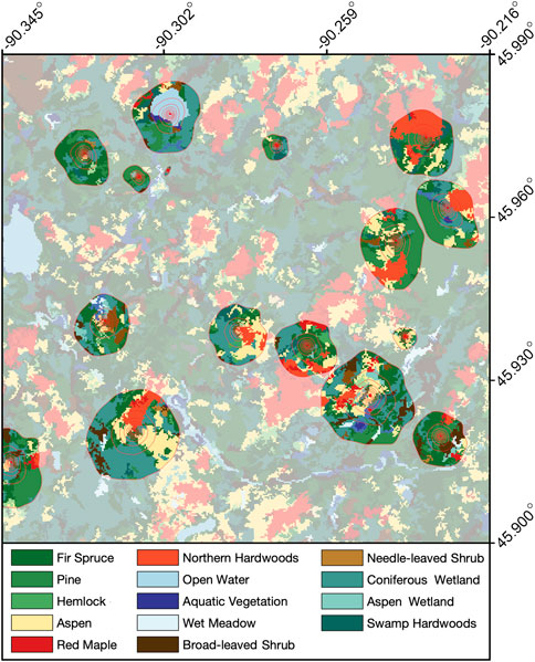
FIGURE 1. Map showing land cover classifications across the 10 × 10 km CHEESEHEAD19 domain. The areas of full color represent the mean flux footprint climatologies of the 17 ISFS towers, while the areas with a partially transparent white shading represent areas outside those footprints.

2.2 Energy balance calculations

Temporal sensible and latent heat fluxes (Eqs 2, 3) from EC towers were calculated as

where $\overline{{\rho }_a}$ (mol m⁻³) is the mean dry air density, c_p (J kg⁻¹ K⁻¹) is specific heat capacity of dry air, w (m s⁻¹) is vertical wind speed, T (K) is dry air temperature, L_v (J kg⁻¹) is latent heat of vaporization, and q (kg kg⁻¹) is specific humidity. The dry air temperature was calculated from the sonic temperature after correction for the effect of water vapor on air density and speed of sound (Schotanus et al., 1983). Overbars correspond to time averages and primes indicate fluctuations about the mean. For temporal fluxes the fluctuation components for w, T, and q were calculated by subtracting the 30-min mean from the instantaneous 20 Hz values (e.g., $w^{\prime }=w-\overline{w}$) on a site-by-site basis. Because some sites experienced directionally-dependent angles of attack, a single (not sectorial) planar fit coordinate rotation was applied to the wind vector for all analyses (except where otherwise stated).

While EC is generally considered a reliable method for measuring fluxes, there are certain limitations and uncertainties. To reduce measurement uncertainty, we applied several standard quality control techniques to the flux measurements. Specifically, we rejected flux intervals based on sensor diagnostic flags, integral turbulence characteristics tests (Foken and Wichura, 1996; Mauder and Foken, 2004), and nonstationarity (Blomquist et al., 2014). Uncertainties related directly to instrument biases (e.g., Frank et al., 2013) were not examined because individual sites lacked the instrument redundancies required to quantify such issues. While such uncertainties are likely to be partially responsible for observed energy balance non-closure, they are not expected to qualitatively change the energy balance forcings investigated herein.

In addition to traditional, temporal EC, we calculated fluxes using both spatial EC and spatio-temporal EC. These were used to test whether spatial forms of EC could better represent the energy balance over heterogeneous ecosystems. They were calculated as

where angle brackets represent spatial averaging and double prime refers to fluctuations around the spatial mean. The key difference between spatial and spatio-temporal EC is in the way the velocity and scalar fluctuation components are calculated. For spatial EC the fluctuation terms are calculated by subtracting 20 Hz values by the 20 Hz spatial mean across all sites (e.g., $w^{″}=w-〈w〉$), resulting in 20 Hz fluxes. For spatio-temporal EC the fluctuation terms are calculated by subtracting 20 Hz values by the 30-min spatial mean across all sites (e.g., $w^{″}=w-〈\overline{w}〉$). For this study the spatial EC fluxes were time-averaged from 20 Hz frequency to 30 min to achieve temporal equivalence in comparisons with temporal and spatio-temporal EC fluxes. Note that timestamps at all sites were continuously monitored and adjusted by a network time protocol software, using a GPS reference clock with a precise pulse-per-second signal. Times are expected to be correct across sites to within 50 microseconds.

One additional term calculated to identify spatial patterns in the surface energy fluxes was dispersive flux. Like spatial EC, it represents a covariance arising from spatial correlations of measurements over space, but is calculated with time-averaged quantities. The term can be added to single-site, temporal EC fluxes to produce a total, spatially averaged covariance (Raupach and Shaw, 1982). It is calculated using the equations:

In the simplest terms, a dispersive flux is the mean spatial flux over a period of time, resulting from spatially localized deviations from the mean flow. Dispersive fluxes represent a portion of the influence of larger-scale atmospheric motions on a flux area; scales that are difficult to measure by a single-site eddy covariance tower. However, this does not account for larger-scale divergence of the mean flows (Metzger, 2018; Morrison et al., 2021; Morrison et al., 2023).

In addition to flux measurements, the ISFS towers of the NSF LAOF were designed to measure the G, S_soil, and S_atmo terms. Soil heat fluxes (G) were measured using heat flux plates (HFT; REBS) installed at a depth (z_p) of 5 cm. The details of this process are described in Oncley et al. (2007). Soil storage (Eq. 8) values in the layer above the heat flux plates were calculated using the equation:

where soil temperature (T_soil) was calculated as the linear average of 4 temperature sensors (TP01; Hukseflux) evenly spaced through the first 5 cm of soil. The soil heat capacity (c_soil) was calculated as a combination of water and dry soil heat capacities ($c_{soil}={\rho }_{water}{q}_{soil}{c}_{water}+{\rho }_{dry\_soil}{c}_{dry\_soil}$) weighted using soil moisture data (EC-5; Decagon) and bulk soil density measurements.

Atmospheric storage of heat from T and q (S_atmo = S_air-T + S_air-q) below the EC flux sensor are represented by the Eqs 9, 10:

where z_m is flux measurement height. For the calculation these integrals were discretized, using T and q measurements at z_m and from additional TRH sensors installed at 2 and 10 m AGL. Unlike soil measurements, T and q properties in the air are variable over short timescales. Therefore, to avoid introducing an unreasonable amount of noise, the T and q time derivatives were calculated as the difference between the means of the first and last 5-min periods of each 30-min flux interval divided by 1,500 s (i.e., 25 min).

At densely forested sites it was expected that some amount of energy would also be stored in plant biomass (S_bio). Therefore, instruments aimed at estimating this additional storage term were deployed. S_bio was estimated from tree temperature measurements obtained at five ISFS sites from September 2019 to April 2020. At each site (NE2, NE3, NE4, SW2, SW4) two Onset Hobo MX-2304 were installed into two different trees at 2 m AGL. S_bio was calculated as

where c_p is the specific heat of wood and dT/dt is the change in temperature over time measured by the temperature sensors and biomass representing the mass of the forest. Biomass was estimated by using Wisconsin DNR forest lidar data to estimate mean tree height for each site (mean tree height = digital surface model–digital elevation model), then estimating diameter at breast height (DBH) from mean tree height using allometric equations and constants specific to the tree species at each site (Desai et al., 2007). Then mean DBH and mean tree height were used to calculate biomass per m² using allometric equations and constants.

2.3 Sensitivity analysis

The evaluation of spatial and spatio-temporal EC was incorporated into a larger sensitivity analysis, which evaluated the influence on energy balance closure of 1) EC type, 2) tower selection, and 3) coordinate rotation. Figure 2 shows all permutations of processing techniques for which H_S and H_L were calculated. The flux calculations influenced no other part of the energy balance equation (i.e., R_N, G, or S). Therefore, we interpreted the improvement to energy balance by observing how Imb varied for each permutation of techniques.

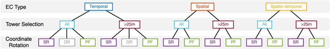
FIGURE 2. Tree diagram showing all permutations of processing techniques tested in the sensitivity analysis. Three EC types (temporal, spatial, and spatio-temporal) were calculated for each of two categories of tower selection (all towers and towers ≥25 m) and three categories of coordinate rotation (single rotation [SR], double rotation [DR], and planar fit [PF]). Note that the double rotation coordinate rotation was only applied to temporal EC.

Preliminary analyses showed that the selection of suitable towers within the tower network can influence the calculated fluxes. Therefore, in the sensitivity analysis we calculated fluxes using 1) all towers and 2) towers ≥25 m AGL.

Coordinate rotation refers to the rotation of the wind vector used to calculate vertical velocity fluctuation used in the flux calculation. Two variations were applied to all EC types–single rotation and planar fit. A third coordinate rotation, a double rotation, was applied to temporal EC. Single rotation refers to an azimuthal rotation into the mean horizontal wind. Double rotation refers to an azimuthal rotation into the mean horizontal wind and a subsequent elevational rotation so that the mean vertical wind speed over 30 min equals zero. This rotation was excluded from both forms of spatial EC because setting $\overline{w}$ = 0 for all sites removes the spatial deviations in w expected to contribute to the spatially-calculated flux. Planar fit is also a double rotation, but one in which the wind vector is rotated onto the plane of the long-term (i.e., over weeks or months) mean wind field (mean crosswind component $\overline{v}$ = 0; but $\overline{w}$ is not necessarily 0). It is generally appropriate in temporal EC when a site has a consistent directionally-dependent angle of attack, because it quantifies vertical wind deviations from the long-term mean (Wilczak et al., 2001).

3 Results

3.1 Temporal energy balance characteristics

During CHEESEHEAD19 the magnitude of the energy imbalance (Imb) varied diurnally (Figure 3F) and seasonally (Figure 4C). Most sites exhibited a distinct diurnal trend of negative Imb at night and larger, positive Imb during the daytime, leading to a net daily positive Imb. Imb also varied across space, with some sites exhibiting characteristically high Imb throughout the experiment while other sites exhibited low Imb (Figure 3F).

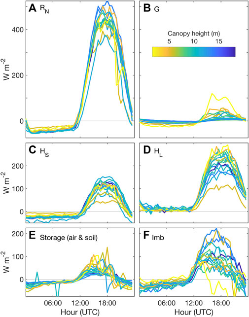
FIGURE 3. Mean diurnal cycle of energy balance components (A) R_N, (B) G, (C) H_S, (D) H_L, (E) storage (combined air and soil), and (F) Imb for each of the 17 eddy covariance sites with lines shaded based on mean canopy height at individual sites. Note that panel dimensions vary to maintain a consistent y-axis energy scale across all panels. The following sign conventions are used to match Eq. 1: in panels a and b positive values indicate downward energy transport, in panels c and d positive values indicate upward energy transport, in panel e positive value indicate energy is going into storage, and in panel f positive values indicate that available energy is greater than turbulent fluxes.

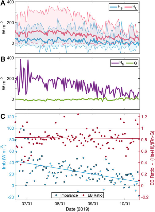
FIGURE 4. Daily mean (A) sensible and latent heat fluxes (shading represents daily range), (B) R_N and G, and (C) Imb and energy balance ratio (with corresponding lines representing least squares fit).

In addition to changing diurnally, the energy balance components changed seasonally (Figure 4C). Positive Imb values decreased throughout the study period from their highest values in June (∼100 W m⁻²) to their lowest values in October (∼0 W m⁻²). These magnitudes correlate with the reduction in R_N throughout the season (Figure 4B). This results in the energy balance ratio staying constant near 0.8 through the seasonal transition (i.e., Imb changes in direct proportion to R_N).

3.2 Spatial energy balance characteristics

An investigation across the flux sites revealed relationships between canopy characteristics (mean canopy height and standard deviation) and energy balance components. Energy balance residual had positive relationships with both canopy height and canopy standard deviation (Figure 5). This appears at least partially because sites with shorter, scrubbier vegetation measured greater ground flux and soil storage, which accounted for a sizable portion of what otherwise would have been residual. This larger G and S_soil appeared to be the result of direct incoming solar radiation reaching the surface, causing greater heating than occurs at the surface under more dense canopies. These sites experienced G + S_soil sums that peaked at ∼150 W m⁻² during the day. This was an order of magnitude higher than peak G + S_soil sums at more densely forested sites.

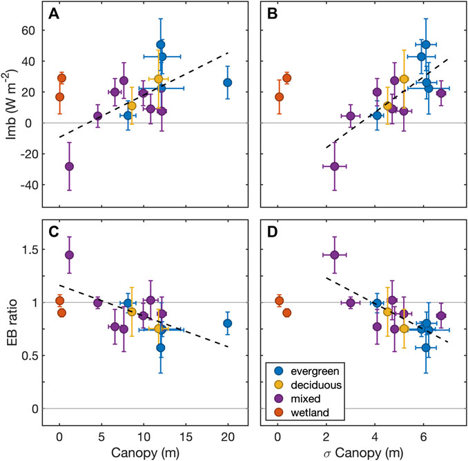
FIGURE 5. Average daily mean Imb [top: (A, B)] and energy balance ratio [bottom: (C, D)] for each ISFS site over the course of the study plotted against mean [left: (A, C)] and standard deviation [right, (B, D)] of canopy heights within the 50% flux footprint climatologies. Regression lines (black dashed) represent regressions through forested sites only (i.e., wetlands excluded).

The investigation into biomass storage revealed that S_bio also varied across the sites, with peak daytime storage ranging from 1 to 11 W m⁻² and a mean of 5 W m⁻² (Figure 6). This represents roughly 6.5% of the mean daytime peak in Imb of 76 W m⁻². This result supports previous findings which show that accounting for biomass heat storage improves energy balance closure, but that it cannot explain the entirety of the missing energy (e.g., Lindroth et al., 2010).

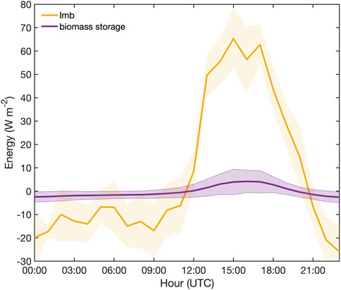
FIGURE 6. Mean diurnal cycle of biomass storage (purple) and Imb (yellow) for five ISFS sites over the 26 days in which tree core temperature measurements overlapped the field campaign. Shaded regions represent standard deviation.

3.3 Sources of energy imbalance

3.3.1 Mesoscale eddies

The array of instrumentation for measuring the atmosphere during CHEESEHEAD19 provided additional benefits for investigating the causes of energy balance non-closure. A range of meteorological and climate variables were examined for their relationship with measured energy imbalance. Atmospheric stability showed one of the strongest relationships, with unstable conditions resulting in strongly positive imbalance and stable conditions showing weakly negative imbalance (Figure 7). This is in line with previous findings (Stoy et al., 2006; Mauder et al., 2010). Most other meteorological variables (e.g., air temperature, vapor pressure deficit, wind speed, wind direction, and pressure) showed no discernible relationship with imbalance (see Appendix).

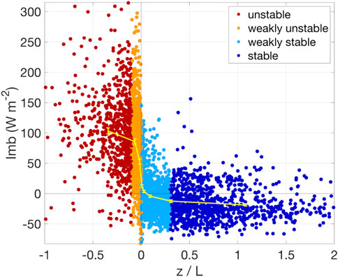
FIGURE 7. Thirty-minute mean Imb vs. atmospheric stability (z/L). Negative z/L values represent unstable conditions and positive values represent stable conditions. Bin averages are displayed in yellow, with error bars representing the 95% confidence interval.

To further investigate the relationship between atmospheric characteristics and energy imbalance we utilized ground-based remote sensing instruments profiling wind and measuring ABL height. These measurements enabled thorough characterizations of the size and scale of eddies in the ABL, as well as provided the ability to calculate vertical profiles of the convective velocity scale ($w_{*}$). This scale roughly translates to the updraft speed of convective thermals in the ABL (Stull, 1988). One leading hypothesis suggests that Imb is caused by the existence of turbulent organized structures or quasi-stationary mesoscale eddies (Mauder et al., 2021). The CHEESEHEAD19 measurements provided observations to test previous LES findings on the role of mesoscale eddies in causing energy balance non-closure.

Figure 8 shows an example of vertical wind speed during a day with high $w_{*}$. The daytime oscillations between updrafts and downdrafts on high $w_{*}$ days showed longer periodicity (10 min to an hour) and greater amplitude (±2 m s⁻¹) than days with low $w_{*}$. The scales of these motions indicated the presence of mesoscale eddies. Therefore, we used $w_{*}$ as a proxy for the strength of mesoscale eddies in further analyses.

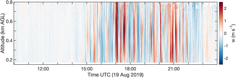
FIGURE 8. Example of vertical winds on a day (19 August 2019) with high $w_{*}$ measured by the vertical stare doppler wind lidar. Mesoscale eddies oscillate between updrafts and downdrafts (±2 m s⁻¹) on time scales ranging from 10 min to an hour during the peak daytime period.

Across the study domain we found that Imb was positively correlated with $w_{*}$ (Figure 9). For this analysis we focused on the afternoon period (1,500–2,100 UTC; ±3 h of solar noon) because that is the time of day which was found to contribute most to the magnitude of daily mean Imb.

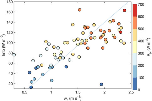
FIGURE 9. Mean daytime (1,500–2100 UTC) Imb vs. mean daytime $w_{*}$. The fit line was calculated using a Deming regression because measurement error is inherent in both Imb and $w_{*}$.

Flux tower cospectra for sensible and latent heat flux were investigated to identify possible causes of the Imb vs. $w_{*}$ relationship (Figure 9). For both high and low $w_{*}$ the mean daytime cospectral curves of sensible and latent heat flux do not go to zero at lower frequencies (Figure 10). This suggests that the 30-min flux interval is excluding some degree of low frequency contribution to the fluxes. We estimated this missing energy by extending the curves linearly to zero and integrating the area under. For sensible heat, this estimated an additional 3.6 and 5.6 W m⁻² for the low and high $w_{*}$ groups, respectively. This magnitude represents 4.9% of the total mean sensible heat flux for the low $w_{*}$ group and 4.2% for the high $w_{*}$ group. For latent heat, the estimated mean missing energy was 3.2 and 11.5 W m⁻² for the low and high $w_{*}$ groups, respectively. This magnitude represents 3.2% of the total mean latent heat flux for the low $w_{*}$ group and 5.1% for the high $w_{*}$ group. While the combined (H_S + H_L) missing energy is larger for the high vs. low $w_{*}$ group (17.1 W m⁻² compared to 6.8 W m⁻²), both represent roughly 10% of the total magnitude of their corresponding Imb.

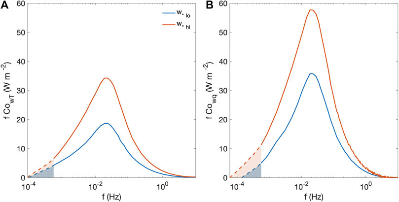
FIGURE 10. Mean daytime (1,500–2100 UTC) cospectral curves for (A) sensible and (B) latent heat fluxes. Red curves represent days with above-median $w_{*}$. Blue curves represent days with below-median $w_{*}$. Shaded regions highlight estimated missing contributions from low frequencies.

Here we demonstrate that free convective conditions (i.e., conditions with a greater preponderance of mesoscale eddies) show larger energy balance residuals. In the next section we investigate whether spatial network of towers deployed in the CHEESEHEAD19 experiment can be used to quantitatively account for the influence of these mesoscale eddies on the surface energy balance of the domain. We specifically investigate two approaches. The first is to calculate dispersive fluxes. The second is to compare heat fluxes calculated using spatial and spatio-temporal EC against traditional temporal EC.

3.3.2 Dispersive fluxes

Dispersive fluxes of sensible and latent heat were calculated as the spatial covariance of the temporal mean values of T and q with w (Eqs. 4, 5). The mean nighttime magnitude of H_{S disp} peaked at 11.7 W m⁻², while daytime values were negligible (Figure 11A). For H_{S disp}, positive values suggests that warm sites exhibit stronger updrafts than cooler sites. For H_{L disp}, the mean nighttime magnitude was negligible, while negative values up to −20 W m⁻² were observed during the daytime (Figure 11A). For H_{L disp}, a negative value means sites with lower humidity have stronger updrafts than more humid sites. Both dispersive fluxes showed a considerable degree of variability, with standard deviation across corresponding hourly bins averaging 22 and 35 W m⁻² over the diurnal cycle, for H_{S disp} and H_{L disp} respectively. However, neither exhibited a seasonal trend.

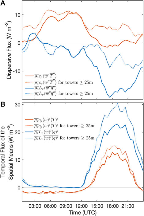
FIGURE 11. Bin median diurnal cycles over the entire study period of (A) H_{S disp} and H_{L disp} and (B) the temporal heat fluxes of the spatial means of w, T, and q. Solid lines represent fluxes calculated using all sites and dashed lines represent fluxes calculated for sites with EC towers at least 25 m AGL. Note that solar noon was at roughly 1800 UTC.

H_{S disp} and H_{L disp} were additionally calculated using only the tall tower sites (towers ≥25 m AGL; 12 of 17 sites). This was done to remove the complexity of interpreting the dispersive fluxes calculated with measurements made at different heights. For H_{S disp}, doing so increased the daytime values to 5 W m⁻², while negligibly changing nighttime values (Figure 11A). For H_{L disp}, the ≥25 m AGL recalculation also reduced the magnitude of the negative daytime dispersive fluxes by roughly half to −8 W m⁻² (Figure 11A).

A converse of the dispersive flux (i.e., the spatial covariance of the temporal means) is the temporal flux of the spatial means. In the Eddy Matrix experiment of Engelmann and Bernhofer (2016) this value was added to spatial EC fluxes to incorporate the domain-wide temporal contributions to the flux over spatially-distributed tower networks. We calculated it here by spatially averaging the 20 Hz values of T, q, and w across all sites and computing a temporal EC flux with those spatial averages. The fluxes calculated using this method resulted in diurnal cycles with the same pattern observed in H_S and H_L of the individual sites (Figures 3C, D), albeit with lower magnitude. For sensible heat flux, the values were slightly negative during the night and peaked at 12.7 W m⁻² during the day (15.1 W m⁻² when isolating towers ≥25 m AGL). For latent heat flux, the values were negligible during the night and peaked at 22.9 W m⁻² during the day (30.4 W m⁻² when isolating towers ≥25 m AGL).

3.3.3 Sensitivity analysis

Figure 12 shows mean diurnal Imb for all permutations of each processing technique in the sensitivity analysis. For this comparison, the temporal fluxes were averaged across all sites and the spatial and spatio-temporal fluxes were averaged over 30-min windows corresponding to the temporal flux intervals. We found that coordinate rotation had a minimal influence on Imb. Changing the coordinate rotation while holding all other processing techniques constant resulted in nearly identical mean diurnal Imb (Figure 12A). The double rotation for temporal EC (not shown) also resulted in near equivalence to single rotation and planar fit.

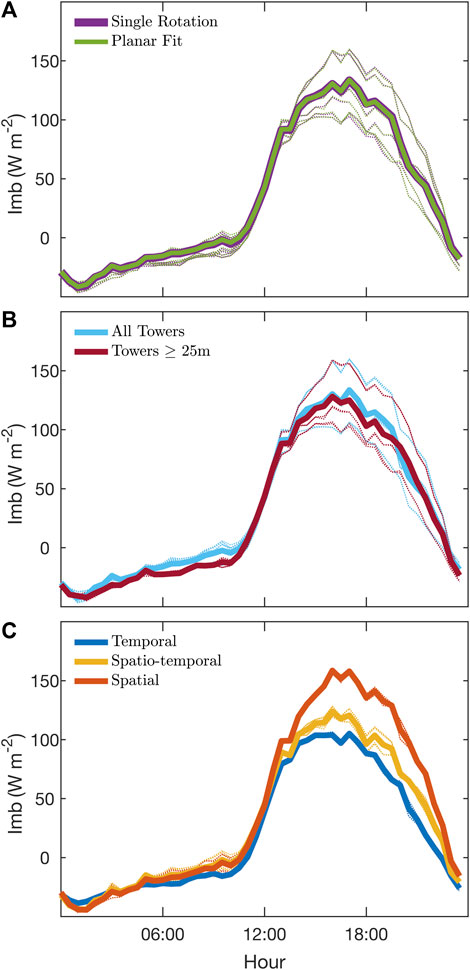
FIGURE 12. Sensitivity analysis ensembles of mean diurnal Imb for (A) coordinate rotation, (B) tower selection, (C) and EC type. Each curve represents the mean across all sites, over the entire study period. Thick curves represent the mean of all permutations for the corresponding variation. Double rotation was not shown because it was not calculated for all EC types.

Within the sensitivity analysis, the largest influence on Imb came from EC type (Figure 12C). The midday period (1,500–2,100 UTC) showed the largest deviations between the EC types. Temporal EC produced the lowest mean diurnal Imb, with peak daytime magnitudes of 87 W m⁻². Spatio-temporal EC produced a higher peak mean daytime Imb of 103 W m⁻², while spatial EC produced the highest peak mean daytime Imb at 137 W m⁻².

While EC type was the most influential of the processing techniques tested in the sensitivity analysis, tower selection did show a minor influence on mean diurnal Imb (Figure 12B). Averaging across all permutations mean Imb was 3.5 W m⁻² lower for EC calculations using towers ≥25 m AGL compared with EC calculations using all towers.

Comparing the influence of the tower selection for different EC types revealed that for temporal EC tower selection had little influence on the mean diurnal Imb (Figure 13). For spatial EC tower selection reduced nighttime Imb to magnitudes comparable to the temporal nighttime Imb, but had little overall influence on daytime mean diurnal Imb magnitudes. Spatio-temporal Imb also showed reduced nighttime magnitudes similar to spatial EC, but additionally showed reduced daytime mean diurnal Imb magnitudes. The difference between peak daytime Imb calculated using spatio-temporal versus temporal EC roughly halved from 20 W m⁻² with all towers to 11 W m⁻² with towers ≥25 m AGL.

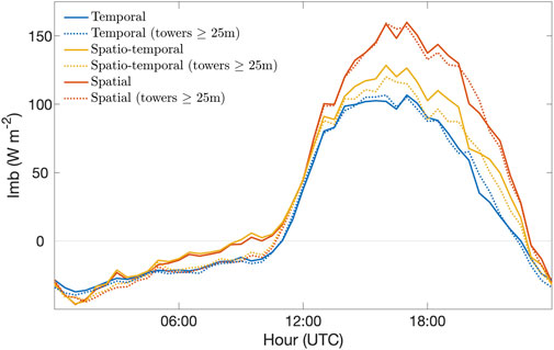
FIGURE 13. Mean diurnal Imb for all the planar fit permutations of EC type (color) and tower selection (solid line: all towers; dashed line: towers ≥25 m AGL).

An additional set of treatments was tested in conjunction with the sensitivity analysis to evaluate the combined EC method of Engelmann and Bernhofer (2016), which was suggested as a possible means of collecting information about larger scale structures. This method combines the spatial EC fluxes (Figure 12C) with the temporal fluxes of the spatial means (Figure 11B). We found that when combining these two components the resultant flux was almost precisely equivalent to the corresponding mean (i.e., across tower selection and coordinate rotation treatments) spatio-temporal fluxes. The standard deviation of difference between the Imb of the combined EC method and spatio-temporal fluxes was less than 1 W m⁻².

4 Discussion

4.1 Energy balance characteristics

A major challenge facing energy balance studies is the different scales at which the measurements are taken. In an idealized scenario the footprints of the H_S, H_L, R_N, and G measurements would precisely match. In practice, there are orders of magnitude difference between them, with H_S and H_L footprints on the order of 100,000 m², R_N roughly 1,000 m², and G roughly 1 m². If the environmental conditions are homogeneous then the different size footprints should not influence the resulting energy balance characterizations. However, when a region is heterogeneous the different measurement footprints can cause mischaracterization of the energy balance for that region. This is particularly difficult when measuring over a forested site, as the installation of a tower generally requires some degree of open space (i.e., a gap in the trees). This means that the downward-facing components of the net radiometer are (at least partially) measuring unforested surfaces (e.g., grass, dirt, road) and will subsequently have a R_N not precisely representative of the flux footprint.

An additional issue related to these open areas is that, at some sites, the soil atop the heat flux plates that measured G received direct sunlight for part of the day. This is expected for grassland sites with limited canopy cover. Such sites have larger downward daytime G than forested sites (e.g., Figure 4B). However, for several forested sites the open patches near the tower resulted in large daytime G measurements uncharacteristic of those measured below an unbroken forest canopy. This is expected to artificially reduced Imb and is likely responsible for the large range across sites of midday Imb seen in Figure 3F.

Our investigation into spatial patterns in energy balance across the domain tested the hypothesis that flux towers with greater footprint heterogeneity would measure greater Imb than more homogeneous sites. The data supported this hypothesis. It was found that sites with higher canopies and more variable canopies (i.e., greater standard deviation) had larger energy balance residuals, both in magnitude and ratio. This corroborated several previous findings, including those of an EC tower network experiment in the Heihe River basin in China which found that in an oasis-desert environment surface heterogeneity within the flux footprints correlated with reduced energy balance closure (Xu et al., 2017; Zhou and Li, 2019). Additionally, across the continental range of sites included in FLUXNET, sites with more heterogeneous land surface (e.g., >σ²_EVI) were found to have greater energy balance residuals (Stoy et al., 2013).

Part of the explanation for the positive relationship between vegetation height and variability appears to be due to measurement footprint discrepancies described above. Sites with shorter vegetation had less canopy cover. This led to larger G measurements, from a greater amount of incoming solar radiation reaching the surface. This G (interpreted as energy departing the exchange surface into the Earth) is subtracted from R_N to get the available energy side of Eq. 1, resulting in a reduction of the magnitude and ratio of the energy balance residual. However, for sites with larger canopies, the small footprint of the G measurement in the open canopy area near the towers was not representative of the entire flux footprints of the H_S and H_L measurements. Therefore, the combined atmospheric heat flux was likely lower for these sites than it would have been under homogeneous conditions matching the G footprint. This also helps explain why the two wetland sites did not match the trends of the forested sites (Figure 5). For the wetland sites the G measurement footprint was generally a better match to the R_N footprint and flux footprints.

The investigation of biomass storage showed that the omission of biomass storage plays a role in the existence of energy balance non-closure. Across five sites and 1 month of measurements, it was found that biomass storage accounted for 6.5% of the magnitude of daytime Imb. On days with large air temperature swings, daytime biomass storage values were frequently between 20 and 40 W m⁻². The relatively large biomass storage magnitudes on such days were due to large biomass dT/dt derivatives (Eq. 11) resulting from the positive relationship between biomass temperature and air temperature. While biomass storage is often omitted from energy balance studies for practical reasons, a thorough accounting of energy balance requires its inclusion. Here we show that while it is not the singular cause of non-closure, it appears to be an important component, especially under certain conditions.

4.2 Mesoscale eddies

The strength of mesoscale eddies was positively correlated with Imb (Figure 9). However, the factors that contribute to Imb appear to act consistently even under conditions with less contribution from mesoscale eddies. This was demonstrated by the consistent energy balance ratio across the seasonal transition (Figure 4C). One example of a proportional cause of non-closure in this dataset was time averaging in the flux calculation.

In traditional EC, time averaging is necessary to provide enough statistical information to calculate a representative flux. Ideally, the window is long enough to include contributions from all scales of turbulent eddies, but short enough to exclude larger scale, non-turbulent contributions (e.g., advection, diurnal cycles). This is the stationarity criterion. While no window length works perfectly for all situations, EC networks (e.g., Ameriflux, NEON, FLUXNET, etc.) generally set 30-min averaging windows as standard.

The failure of cospectral curves in Figure 10 to go to zero at lower frequencies suggests that the 30-min averaging window was responsible for eliminating some actual low frequency contribution to the flux. The magnitude of the missing low frequency contribution was greater on days with more developed mesoscale eddies (i.e., days with high $w_{*}$). However, the percentage of the missing contributions with respect to Imb was roughly equivalent to 10% for both high and low $w_{*}$ conditions. Because 30-min averaging windows are a common standard, this suggests that the high-pass filter caused by the averaging window may be a persistent cause of a small, but non-negligible, fraction of Imb across many field measurement campaigns.

4.3 Dispersive fluxes

Our primary objective of this study was to quantify the energy balance influence and improvements of specific data processing techniques. The unique experimental design of the CHEESEHEAD19 project enabled testing both spatial and spatio-temporal EC, as well as dispersive flux contributions to temporal EC fluxes. It should be noted that the experimental setup notably did not lend itself to addressing all possible causes of non-closure. For example, the lack of flux measurements at multiple heights and the absence of side-by-side towers precluded the calculation of vertical flux divergence and advective fluxes. The omission of these fluxes is expected to contribute to energy balance non-closure (Finnigan et al., 2003; Oncley et al., 2007; Morrison et al., 2021; 2023). Nevertheless, the testing of spatial forms of EC over a domain with the spatial scale of the CHEESEHEAD19 tower network represents a novel scientific endeavor.

Previous studies have suggested that accounting for dispersive flux may reduce energy balance non-closure (Kanda et al., 2004; Mauder et al., 2020; Mauder et al., 2021; Morrison et al., 2023). There are theoretical reasons for including dispersive fluxes. Namely, that they represent one contribution of mesoscale motions to the energy balance that cannot be measured by single EC towers (Mauder et al., 2020; Mauder et al., 2021). Fortunately, this term can be incorporated with straightforward calculations (i.e., Eqs. 6, 7) using data from a flux tower network. Because it relies solely on mean meteorological terms it can also be measured without flux towers, by having a network of basic meteorological stations (Mauder et al., 2008).

The dispersive fluxes calculated using the CHEESEHEAD flux network were relatively small compared to other energy balance components included in the analysis. The hourly bin medians of the diurnal cycle for both H_{S disp} and H_{L disp} (from ≥25 m towers) peaked at roughly 10 W m⁻² and −10 W m⁻² (Figure 11A), respectively, but averaged to 7 and −3.5 W m⁻² over the daily cycle. The existence of relatively small dispersive fluxes agrees with the findings of Morrison et al. (2023), who found that dispersive fluxes accounted for a negligible portion of the surface energy budget. The considerable degree of variability in the dispersive fluxes is potentially due to the variable nature of secondary circulations under different meteorological forcings (Paleri et al., 2022).

The temporal flux of the spatial means (Figure 11B) showed larger magnitude and more consistent diurnal cycle compared to dispersive fluxes. The flux direction in the diurnal cycle matched that of the temporal flux measurements from individual sites, albeit with values an order of magnitude lower. Engelmann and Bernhofer (2016) state that this term may collect information about larger and/or slower structures. However, the theoretical case for this term has not been made. Here we found that the term was equivalent to the difference between spatial and spatio-temporal fluxes. Therefore, it may play a useful role in the decomposition of components contributing to spatio-temporal flux measurements (i.e., those contributions that are purely spatial vs. those that arise from the time-averaging procedure in the spatio-temporal flux calculation).

4.4 Spatial EC

In order to test the ability of spatial forms of EC to improve energy balance closure we conducted a sensitivity analysis in which energy balance residuals were calculated for different permutations of EC type (temporal, spatial, and spatio-temporal), tower selection (all towers, towers ≥25 m), and coordinate rotation (single rotation, double rotation, and planar fit). The inclusion of the latter two categories was to ensure that technical considerations were not responsible for Imb differences observed between EC types. An important consideration in the interpretation of the CHEESEHEAD19 sensitivity analysis is that reduction of energy balance closure does not necessarily correspond to improved (i.e., “truer”) flux measurements. This is because any change that increases H_S or H_L will have the effect of reducing Imb. And there are processing techniques that increase H_S and H_L that may not be theoretically defensible. But when the processing technique is both supported by theory and has the effect of reducing energy balance non-closure it provides a better justification for choosing that specific technique.

The coordinate rotation of the wind vector was found to be the category with the least impact on Imb (Figure 12A). It was observed that averaged over the course of the study period (and across all sites) the difference in Imb between single rotation and planar fit EC fluxes was negligible (<1 W m⁻²). However, a closer inspection of H_S and H_L revealed a range of influences on actual fluxes. Some sites, the ones with relatively minor angle of attack directional dependence, had nearly no difference between single rotation and planar fit fluxes, because the planar fit was effectively orthogonal to gravity just like single rotation. The sites with stronger directional dependence did witness up to 10% differences between the flux measurements calculated using different coordinate rotations. However, except for one site (NW4), the differences were equally distributed around a common mean (i.e., no coordinate rotation showed a consistent bias high or low). This resulted in the long-term analysis of Imb to reveal no impact from coordinate rotation. While further analyses on the specific deviations on Imb under different conditions will be performed, this analysis revealed that the type of coordinate rotation used is not a primary contributor to Imb.

With respect to EC type, we hypothesized that spatial forms of EC would reduce Imb by better incorporating contributions from mesoscale eddies. This hypothesis was informed by an LES analysis which demonstrated this result (Xu et al., 2020). We found that the spatial forms of EC tested in this field experiment did not support the stated hypothesis. In fact, we observed a substantial increase in Imb for spatial EC, averaging 50 W m⁻² greater during peak daytime conditions compared to temporal EC (Figure 12C). This corresponds to the results of Engelmann and Bernhofer (2016), who also observed increased Imb for spatial EC. In addition to spatial EC, we tested spatio-temporal EC fluxes for their ability to improve energy balance closure. We found that this method did improve closure (i.e., reduced Imb) compared to spatial EC, but still produced larger Imb values than temporal EC. The difference between spatio-temporal and temporal EC-derived Imb was reduced when flux calculations were performed using towers of similar height (i.e., the midday difference of 20 W m⁻² with all towers was reduced to 11 W m⁻² when selecting for tall towers; Figure 13). However, the persistently larger Imb for both spatial and spatio-temporal EC under all permutations shows that, under the test conditions, spatial forms of EC did not perform better at balancing the energy budget.

In their experiment, Engelmann and Bernhofer (2016) performed an additional EC technique which they call the combined EC method. For that calculation they added the spatial EC fluxes to the additional flux derived from the temporal covariance of the spatial mean values. This resulted in a large Imb reduction compared to spatial EC and a modest Imb reduction compared to their reference temporal EC fluxes. We also tested this approach and found that while it reduced Imb relative to spatial EC, it still produced Imb values slightly larger than those calculated using temporal EC. Interestingly, we found that the combined EC method of Engelmann and Bernhofer (2016) produced the same values as directly-calculated spatio-temporal fluxes (Eqs. 4, 5). This suggests that the combined EC method is a spatio-temporal flux calculation simply decomposed into its constituent parts (i.e., the spatial and temporal EC terms).

With this in mind, we can see that the spatio-temporal fluxes of the 9-tower Eddy Matrix of Engelmann and Bernhofer (2016) did slightly improve energy balance closure, while the 17-tower spatio-temporal fluxes from the CHEESEHEAD19 showed slightly poorer energy balance closure compared to temporal EC. One possible cause of this is the practical limitations of deploying a tower network over a large, heterogeneous domain, including greater distances between the sites, the variety of land surface types, and the varying flux measurement heights relative to canopy. Such physical characteristics may complicate the ways in which turbulence is measured using spatial and spatio-temporal EC. Indeed, the theoretical requirements for spatial EC suggest that in order for a spatial array of instruments to provide meaningful flux data, the measurements should be collected within a homogeneous turbulence field (Stull, 1988). This requirement would appear more difficult to fulfill in the broad domain of CHEESEHEAD19 compared to the small, idealized setup of Engelmann and Bernhofer (2016). However, such shortcomings (if relevant) would likely be resolved by the inclusion of all terms in the continuity equation, including horizontal advection and vertical flux divergence (Metzger, 2018; Morrison et al., 2021; 2023). Unfortunately, this could not be tested here due to the limitations of the experimental design. In spite of this, the spatial and spatio-temporal EC results from the CHEESEHEAD19 domain often show energy fluxes of similar magnitude compared to temporal EC fluxes. This shows that, at least to some degree, spatial forms of EC are capable of measuring over larger domains.

5 Conclusion

The dense set of multi-scale surface-atmosphere exchange observations collected during the CHEESEHEAD19 field campaign provided a data foundation for evaluating theoretical explanations of surface energy balance non-closure, as well as to evaluate spatial methods for observing the energy balance over a larger domain. In our characterization of energy balance, we found that individual components varied both spatially and temporally. Across the domain, the energy balance residuals were largest for sites with higher canopies, as well as for sites with greater variability in vegetation height. Diurnally, residuals were largest during the afternoon. This coincided with the period when mesoscale motions were strongest. This supports the hypothesis that quasi-stationary mesoscale eddies are an important contributor to the non-closure of the energy balance. Over the seasonal transition from latent heat-dominated summer to sensible heat-dominated fall, the magnitude of Imb decreased steadily. However, the energy balance ratio remained constant at 0.8, which suggested that causes of energy balance had similar influence across seasons. This was demonstrated by the comparison of low frequency flux loss between high and low $w_{*}$ periods, where greater magnitudes of missing energy were found for high $w_{*}$ versus low $w_{*}$ days, but the percentage of total energy fluxes remained constant. This work highlighted that there are multiple causes of energy balance non-closure that influence the budget simultaneously. The more complete expression of terms in the energy balance equation goes part of the way towards explaining the observed energy balance non-closure. These components include below instrument air T and q storage, biomass storage, and domain-wide dispersive fluxes. During the daytime these can regularly sum to 75 W m⁻². Because peak daytime Imb reaches a mean maximum of 140 W m⁻², these additional components compose roughly half of the missing energy. The remainder could potentially be accounted for by including the advective terms in the continuity equation.

The EC network also presented an opportunity to test the effectiveness of using spatial EC to measure energy balance. Spatial EC calculates velocity and scalar fluctuations with respect to the spatial means across the tower network, rather than with respect to the temporal means at each individual tower (like traditional EC). It has been proposed as a potential way to reduce energy balance residuals by incorporating contributions from mesoscale motions better than single-site temporal EC. Here we tested several variations of spatial EC with the CHEESEHEAD19 dataset but found no improvement to energy balance closure. We attribute this, in part, to the challenging measurement requirements. The large distances between towers and the varying surface characteristics of the sites potentially contributed to an incomplete accounting of atmospheric turbulence using these spatial EC methods. While spatial forms of EC did not provide direct improvement to energy balance closure, the benefits of deploying a tower network over a heterogenous ecosystem were clear. Using temporal EC, the magnitude of the energy balance residual across all sites during the daytime ranged roughly 200 W m⁻². Therefore, the deployment of a tower network provided a more complete picture of the energy balance over the ecosystem than could have been achieved by any one site.

CHEESEHEAD19 was a project specifically designed to identify the spatial scales relevant to the Earth’s energy balance. By deploying an EC tower network over a domain the size of a typical model grid cell (10 km × 10 km), the project was well situated to investigate the energy transfers at both meso- and microscales. Here we showed that the spatial heterogeneity of surface fluxes can be large, even over a relatively simple landscape. Such heterogeneities influence the energy balance and, moving forward, warrant a more formal procedure for their accounting into energy budgets.

Data availability statement

The datasets presented in this study can be found in online repositories. The names of the repository/repositories and accession number(s) can be found below: www.eol.ucar.edu/field_projects/cheesehead.

Author contributions

BB conducted analyses and wrote the main manuscript. AD, DD, HK, MM, SM, SP, and LW provided substantial contributions to the acquisition of the data, as well as the conception and design of the analyses presented. DL conducted the biomass storage analysis. All authors contributed to the article and approved the submitted version.

Funding

This project was financially supported by NSF Award 1822420, NSF Award 2313772, Deutsche Forschungsgemeinschaft (DFG) Award 406980118, NSF Award DBI-0752017, NSF Award 1638720, the Department of Energy AmeriFlux Management Project support of the ChEAS core site cluster, NOAA Grant NA17AE1623, NSF Award 1918850, and the University of Wisconsin–Madison Office of the Vice Chancellor for Research and Graduate Education with funding from the Wisconsin Alumni Research Foundation. BB was additionally supported by the NOAA Physical Sciences Laboratory.

Acknowledgments

We would like to acknowledge operational, technical, and scientific support provided by NCAR’s Earth Observing Laboratory, sponsored by the National Science Foundation. We would also like to acknowledge the National Ecological Observatory Network (NEON)—a program sponsored by the National Science Foundation and operated under cooperative agreement by Battelle. This material is based in part upon work supported by the National Science Foundation through the NEON Program.

Conflict of interest

The authors declare that the research was conducted in the absence of any commercial or financial relationships that could be construed as a potential conflict of interest.

Publisher’s note

All claims expressed in this article are solely those of the authors and do not necessarily represent those of their affiliated organizations, or those of the publisher, the editors and the reviewers. Any product that may be evaluated in this article, or claim that may be made by its manufacturer, is not guaranteed or endorsed by the publisher.

References

Appendix A

Meteorological variables were examined for their relationship to energy imbalance (Figure A1). With the exception of stability (Figure 7), basic meteorological variables generally did not show a clear relationship with imbalance. Air temperature showed a slight positive relationship (Figure A1a). However, it was found to be dependent on temperature’s relationship with stability, with warm daytime temperatures typically corresponding with unstable conditions, and cooler nighttime air typically corresponding with stable conditions. Vapor pressure deficit (VPD), wind speed, wind direction, and atmospheric pressure all had no relationship with measured imbalance (Figure A1b–e). A timeseries of 30-min mean Imb (Figure A1f) was included to show the diurnal range of Imb over the study period. It was found that the diurnal range was largest in the summer months (July/Aug) when diurnal stability oscillations were largest. The diurnal range in Imb was lower in the fall months (Sep/Oct) when diurnal stability oscillations were of a lower magnitude.

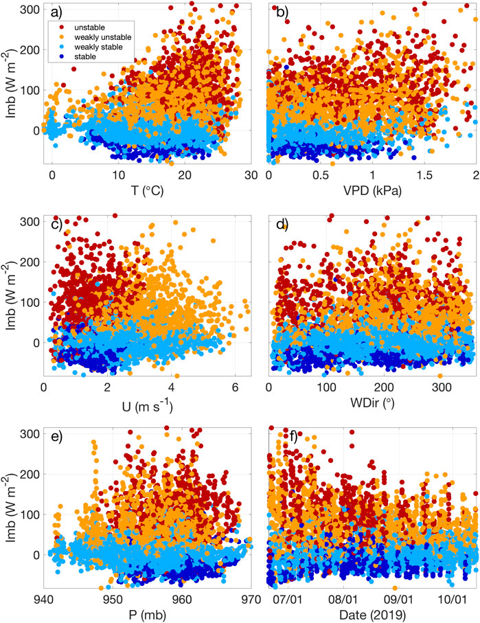
FIGURE A1. Thirty-minute, all-site mean Imb vs. (A) air temperature, (B) vapor pressure deficit, (C) wind speed, (D) wind direction, (E) pressure, and (F) date. Marker color represents stability (i.e., unstable < − 0.1 < weakly unstable <0 < weakly stable <0.3 < stable).

References

Blomquist, B. W., Huebert, B. J., Fairall, C. W., Bariteau, L., Edson, J. B., Hare, J. E., et al. (2014). Advances in air-sea CO2 flux measurement by eddy correlation. Boundary-Layer Meteorol. 152, 245–276. doi:10.1007/s10546-014-9926-2
Butterworth, B. J., Desai, A. R., Townsend, P. A., Petty, G. W., Andresen, C. G., Bertram, T. H., et al. (2021). Connecting land–atmosphere interactions to surface heterogeneity in CHEESEHEAD19. Bull. Am. Meteorol. Soc. 102, E421–E445. doi:10.1175/BAMS-D-19-0346.1
Desai, A. R., Moorcroft, P. R., Bolstad, P. v., and Davis, K. J. (2007). Regional carbon fluxes from an observationally constrained dynamic ecosystem model: impacts of disturbance, CO2 fertilization, and heterogeneous land cover. J. Geophys. Res. Biogeo. 112 (G1), G01017. doi:10.1029/2006JG000264
Desjardins, R. L. (1985). Carbon dioxide budget of maize. Agric. For. Meteorol. 36, 29–41. doi:10.1016/0168-1923(85)90063-2
Eder, F., Schmidt, M., Damian, T., Träumner, K., and Mauder, M. (2015). Mesoscale eddies affect near-surface turbulent exchange: evidence from lidar and tower measurements. J. Appl. Meteorol. Climatol. 54, 189–206. doi:10.1175/JAMC-D-14-0140.1
Engelmann, C., and Bernhofer, C. (2016). Exploring eddy-covariance measurements using a spatial approach: the eddy Matrix. Boundary-Layer Meteorol. 161, 1–17. doi:10.1007/s10546-016-0161-x
Finnigan, J. J., Clement, R., Malhi, Y., Leuning, R., and Cleugh, H. A. (2003). A Re-evaluation of long-term flux measurement techniques Part I: averaging and coordinate rotation. Boundary-Layer Meteorol. 107, 1–48. doi:10.1023/a:1021554900225
Foken, T. (2008). The energy balance closure problem: an overview. Ecol. Appl. 18, 1351–1367. doi:10.1890/06-0922.1
Foken, T., and Wichura, B. (1996). Tools for quality assessment of surface-based flux measurements. Agric. For. Meteorol. 78, 83–105. doi:10.1016/0168-1923(95)02248-1
Frank, J. M., Massman, W. J., and Ewers, B. E. (2013). Underestimates of sensible heat flux due to vertical velocity measurement errors in non-orthogonal sonic anemometers. Agric. For. Meteorol. 171–172, 72–81. doi:10.1016/j.agrformet.2012.11.005
Franssen, H. J. H., Stöckli, R., Lehner, I., Rotenberg, E., and Seneviratne, S. I. (2010). Energy balance closure of eddy-covariance data: a multisite analysis for European FLUXNET stations. Agric. For. Meteorol. 150, 1553–1567. doi:10.1016/j.agrformet.2010.08.005
Kanda, M., Inagaki, A., Letzel, M. O., Raasch, S., and Watanabe, T. (2004). LES study of the energy imbalance problem with eddy covariance fluxes. Boundary-Layer Meteorol. 110, 381–404. doi:10.1023/B:BOUN.0000007225.45548.7a
Lee, X., and Black, T. A. (1993). Atmospheric turbulence within and above a douglas-fir stand. Part II: eddy fluxes of sensible heat and water vapour. Boundary-Layer Meteorol. 64, 369–389. doi:10.1007/BF00711706
Lehner, M., Rotach, M. W., Sfyri, E., and Obleitner, F. (2021). Spatial and temporal variations in near-surface energy fluxes in an Alpine valley under synoptically undisturbed and clear-sky conditions. Q. J. R. Meteorol. Soc. 147 (737), 2173–2196. doi:10.1002/qj.4016
Lindroth, A., Mölder, M., and Lagergren, F. (2010). Heat storage in forest biomass improves energy balance closure. Biogeosciences 7, 301–313. doi:10.5194/bg-7-301-2010
Mahrt, L. (1998). Flux sampling errors for aircraft and towers. J. Atmos. Ocean. Technol. 15, 416–429. doi:10.1175/1520-0426(1998)015<0416:FSEFAA>2.0.CO;2
Mauder, M., Desjardins, R. L., Pattey, E., Gao, Z., and van Haarlem, R. (2008). Measurement of the sensible eddy heat flux based on spatial averaging of continuous ground-based observations. Boundary-Layer Meteorol. 128, 151–172. doi:10.1007/s10546-008-9279-9
Mauder, M., Desjardins, R. L., Pattey, E., and Worth, D. (2010). An attempt to close the daytime surface energy balance using spatially-averaged flux measurements. Boundary-Layer Meteorol. 136, 175–191. doi:10.1007/s10546-010-9497-9
Mauder, M., and Foken, T. (2004). Documentation and instruction manual of the eddy covariance software package TK2. Universitat Bayreuth, Abt. Mikrometeorologie Arbeitsergebnisse 26, 44. ISSN 1614-8924. doi:10.5194/bg-5-451-2008
Mauder, M., Foken, T., and Cuxart, J. (2020). Surface-energy-balance closure over land: a review. Boundary-Layer Meteorol. 177, 395–426. doi:10.1007/s10546-020-00529-6
Mauder, M., Ibrom, A., Wanner, L., De Roo, F., Brugger, P., Kiese, R., et al. (2021). Options to correct local turbulent flux measurements for large-scale fluxes using an approach based on large-eddy simulation. Atmos. Meas. Tech. 14, 7835–7850. doi:10.5194/amt-14-7835-2021
Metzger, S. (2018). Surface-atmosphere exchange in a box: making the control volume a suitable representation for in-situ observations. Agric. For. Meteorol. 255, 68–80. doi:10.1016/j.agrformet.2017.08.037
Morrison, T., Calaf, M., Higgins, C. W., Drake, S. A., Perelet, A., and Pardyjak, E. (2021). The impact of surface temperature heterogeneity on near-surface heat transport. Boundary-Layer Meteorol. 180 (2), 247–272. doi:10.1007/s10546-021-00624-2
Morrison, T. J., Calaf, M., and Pardyjak, E. R. (2023). A full three-dimensional surface energy balance over a desert playa. Q. J. R. Meteorol. Soc. 149, 102–114. doi:10.1002/qj.4397
Oncley, S. P., Foken, T., Vogt, R., Kohsiek, W., DeBruin, H. A. R., Bernhofer, C., et al. (2007). The Energy Balance Experiment EBEX-2000. Part I: overview and energy balance. Boundary-Layer Meteorol. 123, 1–28. doi:10.1007/s10546-007-9161-1
Paleri, S., Desai, A. R., Metzger, S., Durden, D., Butterworth, B. J., Mauder, M., et al. (2022). Space-scale resolved surface fluxes across a heterogeneous, mid-latitude forested landscape. J. Geophys. Res. Atmos. 127. doi:10.1029/2022JD037138
Raupach, M. R., and Shaw, R. H. (1982). Averaging procedures for flow within vegetation canopies. Boundary-Layer Meteorol. 22, 79–90. doi:10.1007/BF00128057
Schotanus, P., Nieuwstadt, F. T. M., and de Bruin, H. A. R. (1983). Temperature measurement with a sonic anemometer and its application to heat and moisture fluxes. Boundary-Layer Meteorol. 26, 81–93. doi:10.1007/bf00164332
Schröter, M., Bange, J., and Raasch, S. (2000). Simulated airborne flux measurements in a LES generated convective boundary layer. Boundary-Layer Meteorol. 95, 437–456. doi:10.1023/A:1002649322001
Steinfeld, G., Letzel, M. O., Raasch, S., Kanda, M., and Inagaki, A. (2007). Spatial representativeness of single tower measurements and the imbalance problem with eddy-covariance fluxes: results of a large-eddy simulation study. Boundary-Layer Meteorol. 123, 77–98. doi:10.1007/s10546-006-9133-x
Stoy, P. C., Katul, G. G., Siqueira, M. B. S., Juang, J., Novick, K. A., McCarthy, H. R., et al. (2006). Separating the effects of climate and vegetation on evapotranspiration along a successional chronosequence in the southeastern US. Glob. Chang. Biol. 12, 2115–2135. doi:10.1111/j.1365-2486.2006.01244.x
Stoy, P. C., Mauder, M., Foken, T., Marcolla, B., Boegh, E., Ibrom, A., et al. (2013). A data-driven analysis of energy balance closure across FLUXNET research sites: the role of landscape scale heterogeneity. Agric. For. Meteorol. 171–172, 137–152. doi:10.1016/j.agrformet.2012.11.004
Stull, R. B. (1988). An introduction to boundary layer meteorology. Dordrecht: Springer Netherlands. doi:10.1007/978-94-009-3027-8_1
Taylor, G. I. (1938). The spectrum of turbulence. Proc. R. Soc. Lond. Ser. A - Math. Phys. Sci. 164, 476–490. doi:10.1098/rspa.1938.0032
Twine, T. E., Kustas, W. P., Norman, J. M., Cook, D. R., Houser, P. R., Meyers, T. P., et al. (2000). Correcting eddy-covariance flux underestimates over a grassland. Agric. For. Meteorol. 103, 279–300. doi:10.1016/S0168-1923(00)00123-4
Wilczak, J. M., Oncley, S. P., and Stage, S. A. (2001). Sonic anemometer tilt correction algorithms. Boundary-Layer Meteorol. 99, 127–150. doi:10.1023/a:1018966204465
Wilson, K., Goldstein, A., Falge, E., Aubinet, M., Baldocchi, D., Berbigier, P., et al. (2002). Energy balance closure at FLUXNET sites. Agric. For. Meteorol. 113, 223–243. doi:10.1016/S0168-1923(02)00109-0
Xu, K., Sühring, M., Metzger, S., Durden, D., and Desai, A. R. (2020). Can data mining help eddy covariance see the landscape? A large-eddy simulation study. Boundary-Layer Meteorol. 176, 85–103. doi:10.1007/s10546-020-00513-0
Xu, Z., Ma, Y., Liu, S., Shi, W., and Wang, J. (2017). Assessment of the energy balance closure under advective conditions and its impact using remote sensing data. J. Appl. Meteorol. Climatol. 56, 127–140. doi:10.1175/JAMC-D-16-0096.1
Zhou, Y., and Li, X. (2019). Energy balance closures in diverse ecosystems of an endorheic river basin. Agric. For. Meteorol. 274, 118–131. doi:10.1016/j.agrformet.2019.04.019