Unified Scaling Law for Earthquakes: Space-Time Dependent Assessment in Friuli-Venezia Giulia Region

Introduction

Capturing the main features of seismicity in a region is not an easy task. While average properties of earthquakes occurrence over large areas can be defined in pretty robust way, when zooming to a smaller territory, the specific features from limited data sets may prevail, and space and time regularities may be lost. Due to heuristic limitations, the smaller is the region and data time span, the less representative (and verifiable) is the resulting seismicity “portrait,” with obvious consequences on earthquake hazard assessments and forecasting. Therefore in this study we aim to analyze, within the Friuli Venezia Giulia region (Northeastern Italy) and surrounding areas, a set of quantitative measures of seismic activity, which have been investigated also in other regions worldwide, so as to verify their possible similarity/generality and identify their peculiar features.

The study region is located at the Alps-Dinarides transition, along the compressional belt that marks the northern edge of Adria micro-plate; earthquakes in the region are shallow, mostly up to 10–15 km depth, and are prevalently of thrust type to the west and strike-slip to the east (Bressan et al., 2018 and references therein). Northeastern Italy is prone to large earthquakes occurrence (e.g., Gorshkov et al., 2009); the rather high seismic hazard in the region is testified by the several destructive events with occurred in the past, the most recent one being the M6.4 1976 Friuli earthquake (Slejko et al., 1999). However, the instrumental seismic activity recorded since then prevalently consists of low to moderate earthquakes, only sporadically exceeding magnitude 4.0, and with the largest recorded event having magnitude 5.6.

Several efforts have been already devoted to explore the different components of seismicity in the study region, namely the clustering properties (Peresan and Gentili, 2018, 2020; Varini et al., 2020) as well as the temporal variability of background seismicity component (Benali et al., 2020). Here we investigate changes in seismicity as a whole, without differentiating between clustered and background components. At the same time, the proposed analysis aims to account for the main geological and tectonic features of the territory under investigation, by assessing and cross-comparing the temporal variability of seismic dynamics within sub-regions sharing a common tectonic setting, based on seismic districts defined by Bressan et al. (2019).

In order to quantify the changes of observed seismicity in the time-space-energy domain, we make use of different parameters, including classical inter-event times and Benioff strain release (Benioff, 1951). To capture both variability and scaling properties of seismic energy release, we resort to the Unified Scaling Law for Earthquakes (USLE), which generalizes the Gutenberg-Richter (GR) relationship making use of the fractal distribution of earthquake sources in a seismic region (Kossobokov and Mazhkenov, 1988, 1989; Bak et al., 2002; Kossobokov, 2020). In particular, besides the space-time variability of seismicity rate (A), earthquake magnitude exponent (B), and fractal dimension of epicenter loci (C), we consider the time series of the USLE control parameter, η (Kossobokov and Nekrasova, 2017; Kossobokov and Nekrasova, 2019).

An estimation of USLE coefficients for seismic hazard assessment at different space scales, namely from the local scale of FVG region and up to the national scale of Italy, was already performed by Nekrasova et al. (2011). This study, instead, focuses on the temporal variations of USLE parameters, rather than on their average time-independent estimates, with the aim to get new insights in the evolving dynamics of seismicity in different areas of FVG. Based on time-dependent estimates of USLE parameters, as well as on classical inter-event times and Benioff strain release, the time intervals of rather uniform seismic activity are identified for each of the investigated sub-regions; the features of seismicity, for different sub-regions and time windows, are then compared and their statistical significance is assessed by the Kolmogorov-Smirnov test. We anticipate that our analysis highlights significant differences and a number of changes in seismic regimes within the three outlined areas. Specifically, the long-term trend of seismic energy release is found to be different prior and after the occurrence of the largest main shocks within the related sub-region, evidencing non-stationary features of seismic activity that should be factored in seismic hazard assessment. Moreover the USLE coefficients in FVG sub-regions are found to be time-dependent and correlated, displaying interesting patterns in the dynamics of seismicity, which could be related with major earthquakes, as illustrated in some detail in Supplementary Material. Thus, the identified regions and time intervals, with homogeneous features of seismic activity, may provide valuable information for time-dependent seismic hazard assessment and may guide areas selection for earthquake forecasting.

Methods

The seismic dynamics of the territory under investigation is characterized in terms of several moving averages, including 1) the inter-event time, τ, dual to seismic rate; 2) the Benioff strain release, Ʃ (Benioff, 1951) (i.e., the sum of square root of energy, thus, proportional to 10^0.75M) 3) the Unified Scaling Law for Earthquake (USLE) control parameter, η and 4) the USLE parameters values estimated for the moving sexennial time intervals.

In agreement with earlier studies (e.g., Bak et al., 2002; Christensen et al., 2002) on the waiting times T between earthquakes with magnitude greater than M, occurring within a range L, the USLE generalizes the Gutenberg–Richter law (Gutenberg and Richter, 1944), and it provides the rate of occurrence N(M,L) defined as:

where N(M,L) is the expected annual number of earthquakes of magnitude M within an earthquake prone area of diameter L; A, B, and C are constants. A and B characterize the annual rate of magnitude 3.5 events and the magnitude exponent respectively, which are analogous to the a- and b-values in the Gutenberg–Richter relationship (GR), while C estimates the fractal dimension df of the epicenters' loci at the site (Nekrasova and Kossobokov, 2005).

The accumulated data on hypocenters provides enough evidence for assuming that locally seismic locus generating earthquakes might have a self-similar structure of fractures of different size (e.g., Kossobokov and Mazhkenov, 1988; Bak et al., 2002). The multiscale analysis involved in evaluation of the USLE coefficients at a given site, where the count of events is performed in a set of cascading squares (i.e., a “telescope”), combines recurrences for earthquakes obtained from enveloping areas of different size, so as to get enough statistics on larger magnitude shocks from larger territories around, for a reliable confident estimation of scaling.

The results of global and regional studies (Kossobokov and Mazhkenov, 1989; Bak et al., 2002; Nekrasova and Kossobokov, 2002; Nekrosova and Kossobokov, 2003; Nekrosova and Kossobokov, 2005; Nekrasova et al., 2011; Parvez et al., 2014; Nekrasova et al., 2016; Nekrasova et al., 2015) confirm the validity of the USLE at different scales of analysis. The definition of the scales based on the preliminary analysis of the quality of data, the research goal, length dimensions of the regions under investigation and the objects of the investigation in the regions.

We can characterize the seismic rate in terms of USLE used the control parameter η:

where τ is the time between two successive earthquakes, M is the magnitude of the second one, L is the distance between them, B and C the Global USLE values. Bak et al. (2002) provide a physical viewpoint on USLE: “To understand the Unified Law for Earthquakes, it is essential to see what the value of x represents. The quantity L^df · S^−b in the scaling function represents the average number of earthquakes per unit time, with seismic moment greater than S occurring in the area size L × L. Therefore, x is a measure of the number of earthquakes happening within a time interval T. The Unified Law states that the distribution of waiting times between earthquakes depends only on this value.” Here x is equivalent to the control parameter η, and the USLE states that the distribution of inter-event times depends only on the value of the variable η.

The Scaling coefficient estimation (SCE) algorithm (Nekrasova et al., 2015) is used to obtain the values of USLE coefficients. For a fine scale analysis, timely fit to the latest and best data registration period, from 1995 up to now, the OGS catalog permits calculation of the USLE parameters making use of the five bisecting steps of the spatial hierarchy, from the linear size L₀ = 1/2° down to L₄ = 1/32°. In addition, we also consider the global values of USLE (ABC_GV) parameters estimated by Nekrasova and Kossobokov (2019) to characterize the seismicity rate over the long time interval.

Data

Earthquake data used in this study are published as monthly OGS bulletins (OGS, 2019), which are available via the following website http://www.crs.inogs.it/bollettino/RSFVG/. A general overview of data made available by the Friuli-Venezia Giulia (FVG) seismometric network, including the network characteristics, main changes related to network geometry and space-time completeness of the OGS catalog, is provided by Peruzza et al. (2015). A detailed analysis of data completeness in space and time is carried out in Peresan and Gentili (2018); based on their data analysis, we have selected the space-time and magnitude interval where data uniformly complete. Specifically, in our study, we used all earthquakes with duration magnitude M_d ≥ 2.0, recorded during the time interval 1995/1/1–2019/3/21, and located within one of the three FVG sub-regions – Area 1 (A1), Area 2 (A2) and Area 3 (A3), outlined accounting for the tectonic setting of the study region, as shown in Figure 1.

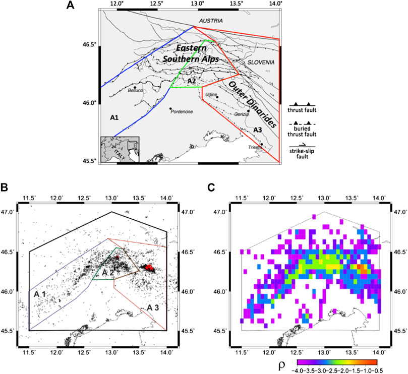
FIGURE 1. The spatial data distribution based on OGS catalog, 1/1/1995–21/03/2019 (A) Map of tectonic lineaments after Bressan et al. (2018) and A1, A2 and A3 sub-regions borders (blue, green and red polygons); (B) M_d ≥ 2.0 earthquakes, the area of uniform completeness (black polygon) and the epicenters of the two largest (M_d ≥ 5.0) earthquakes from the considered catalog (red stars); (C) the empirical density distribution function of seismic activity, cells size 1/16° × 1/16°.

The A1, A2 and A3 sub-regions are formed as combinations of 10 out of 11 FVG seismic districts as defined in Bressan et al. (2018; 2019). The map of the 11 seismic districts of the Friuli Venezia Giulia Region is provided as Supplementary Material S1. Specifically: area A1 is the combination of ALP, CL, AMP and FOA districts; area A2 is the combination of MN, TOC and GE districts and area A3 is the combination of TAR, BOV and BA districts. The PL district is not considered in our analysis, due to its very low level of seismic activity (less than one event per year with magnitude above 2.0). The coordinates of the three sub-regions are provided in Supplementary Table S1.

OGS catalog reports 6640 earthquakes with duration magnitude M_d ≥ 2.0 in the time span from 1995/1/1 to 2019/03/21. The epicenters of 3,011 seismic events fall within the selected sub-regions and 3,629 out of them (Figure 1B). Table 1 lists the OGS catalog earthquake statistics information for the three selected FVG sub-regions and the b-value of the sub-regions earthquakes sets. The time series of earthquakes magnitude, latitude and longitude vs. time, within each of the three Friuli-Venezia Giulia sub-regions, are provided in Supplementary Figure S2.1, along with the Gutenberg-Richter plots of the cumulative number of earthquakes in the different sub-regions (Supplementary Figures S2.2 and S2.3), which allow to verify the magnitude completeness of the data (e.g., according to Mignan and Woessner, 2012).

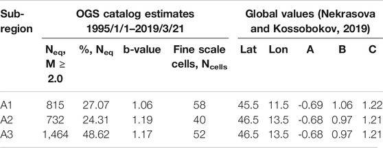
TABLE 1. The three selected Friuli-Venezia Giulia sub-regions data.

The spatial data distribution of events from OGS catalog and the borders of the three selected sub-regions are mapped in Figure 1B, while Figure 1C shows the empirical density distribution ρ of the OGS catalog data obtained from the regular geographic grid cells with size 1/16° × 1/16°. The temporal variability of seismicity rate parameters is compared with the occurrence of the largest earthquakes reported in the considered catalog. Although the FVG region and its surroundings experienced several destructive earthquakes in the past, including the 1976 Friuli earthquake; however, recent seismicity is characterized only by low to moderate magnitude events. The principal earthquakes occurred since 1977 are the 1998 April 12 (M_d 5.6) earthquake and the 2004 July 12 (M_d 5.1). Table 2 lists the information about these principal earthquakes. These events are marked as red stars in Figure 1B.

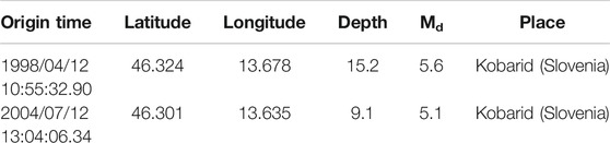
TABLE 2. The two largest earthquakes in Friuli-Venezia Giulia region from 1995 to 2019.

Results

We investigate the changes in seismic regime during the time period from 1995 to 2019 for the three sub-regions (A1, A2 and A3) of the FVG territory (Figure 1A). To quantify the temporal variation of seismicity within each sub-region, we consider the following parameters as a function of time: the inter-event times τ, the cumulative strain release Ʃ, the coefficients A, B, C of the USLE and USLE control parameter η. The empirical cumulative distribution functions of inter-event time τ and Benioff strain release Σ for the entire FVG Region and its three sub-regions are presented in Figure 2. Each distribution can be characterized by the γ-values of the best fit trend. Specifically, the γ-values of the natural exponential trend fit for τ p(>t) = αexp (−γτ) are estimated as 0.48 (R² = 0.96), 0.064 (R² = 0.98), 0.048 (R² = 0.88), and 0.065 (R² = 0.83) in FVG, A1, A2, and A3, respectively. Actually, the best trend fit of τ in A3 sub-region appears to be logarithmic: p(>t) = −0.091 ln(τ) + 0.41 (R² = 0.98). The γ-values for the best power law trend fit for Σ, p(>Σ) = αΣ^−γ, are estimated as 1.23, 1.598, 1.407, 1.586 in FVG, A1, A2, and A3, respectively (R² = 0.98 for all the four cases). LogΣ is a linear function of magnitude M, therefore the distribution of Benioff strain release (Figure 2B) differs from Gutenberg-Richter relation in the abscissa scale only. As is evident from Σ definition, which is proportional to 10^0.75M, the γ-values for Σ are well in agreement with the Gutenberg-Richter the b-values (Table 1).

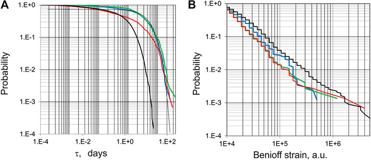
FIGURE 2. Empirical cumulative distribution functions of (A) inter-event time (τ, in days), (B) Benioff strain release (Ʃ, in arbitrary units, a. u.), for M_d ≥ 2.0 events, over the entire FVG territory (1995–2019) and the three sub-regions. Notes: FVG – black line, A1 sub-region – blue line, A2 sub-region – green line; A3 sub-region – red line.

The sample size of the four regions considered may allow further comparison of the γ-values with “q-exponential” or “q-logarithmic” functions of Non-Extensive Statistical Physics (Tsallis, 1988), as is done by (Chochlaki et al., 2018) for most of the 50 regions of the Globe. However, at this time the high R-squared values of the trend fits presented here make us to believe that in case of FVG Region and its sub-regions the Boltzmann–Gibbs theory of additivity might apply, an aspect to be further investigated in the future.

Inter-Event Time τ Temporal Variability

Figure 3 shows the moving averages of inter-event time 〈τ〉 vs. the original event time for A1 (blue line), for A2 (green line) and for A3 (red line) sub-regions. The red trend-line for seismic events in A3 displays two dropping connected with aftershocks of M_d = 5.6 1998 and M_d = 5.1 2004 Kobarid (Slovenia) events.

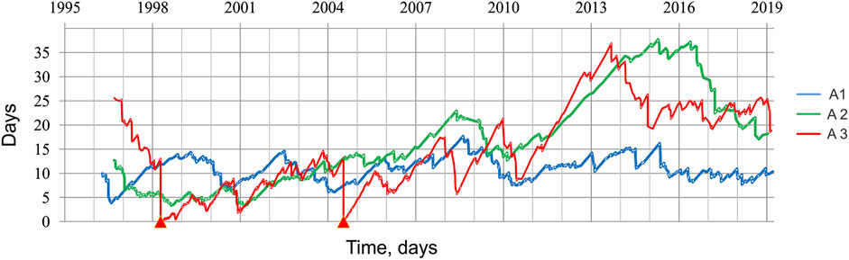
FIGURE 3. Inter-event time (τ, in days) vs. earthquake origin time, for the three sub-regions of FVG territory (1995–2019). A1 – blue line, moving average for 50 earthquakes; A2 – green line, moving average for 50 events; A3 – red line, moving average for 25 earthquakes. The origin time of the two principal earthquakes (Table 2) are marked with red triangles on the origin time scale.

Table 3 lists the linear fit intervals of 〈τ〉 values shown in Figure 3, for each of the three FVG sub-regions; the inspection of linear fit intervals, in fact, may reveal clustered irregularity of the seismic dynamics in the study area. The time intervals for linear fit are determined in a iterative way, namely changing the beginning/ending times until the best fit is obtained (by least squares); the start/end times listed in Table 3 correspond to the occurrence of the specific seismic events that bound the time interval with the best linear fit. Specifically, no evident linear trends can be identified for 〈τ〉 time variations in A1 sub-region. On the other side, within the A2 sub-region, 〈τ〉 time variations display different trends: a decreasing linear trend from June 08, 1998 to March 24, 2017, with the rate of decay of the seismic rate about −1.64 per year and the coefficient of determination R² = 0.91; a rising linear trend of seismic rate from March 24, 2017 to January 15, 2019 (i.e. up to the end OGS catalog), with the rate of 3.5 per year (R² = 0.72). Similarly, within the A3 sub-region the 〈τ〉 time function displays two seismic rate decays: one form August 25, 1998 to July 12, 2004, and another from July 12, 2004 to December 07, 2014, with rates -1.97 per year (R² = 0.80) and -2.81 per year (R² = 0.86) respectively; in A3 there is no evident trend of 〈τ〉 since 2015.

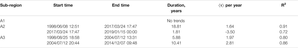
TABLE 3. The moving average interevent time 〈τ〉 trend lines stable intervals for the three FVG sub-regions (1995–2019).

Benioff Strain Release Ʃ Time Changes

Figure 4 shows the cumulative Benioff strain release vs. earthquake origin time, Ʃ(t), for the three FVG sub-regions. As in Figure 3 the origin time of the principal earthquakes is marked by red triangles. We may observe that, while the curve associated with A1 (blue) and A2 (green) sub-regions increase steadily, the red curve associated to the A3 sub-region displays evident jumps corresponding to both principal shocks, mostly reflecting the increased seismicity during aftershocks sequences.

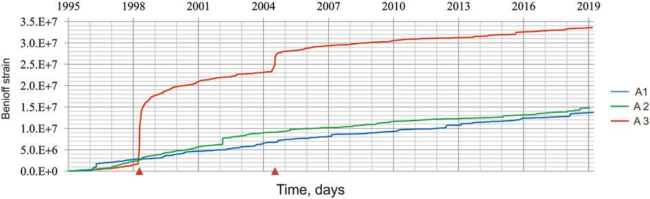
FIGURE 4. The cumulative Benioff strain release Ʃ vs. earthquake origin time for three FVG sub-regions (1995–2019). The color code is the same as in Figure 3: area A1 – blue line, A2 – green line, A3 – red line. The origin time of the two principal earthquakes (Table 2) are marked with red triangles on the origin time scale.

Table 4 lists the linear fit intervals of Ʃ(t) function for the three FVG sub-regions, shown in Figure 4. The time intervals listed in Table 4 are determined following the same procedure applied for 〈τ〉; the start/end times correspond to the first/last earthquakes that bound the intervals providing the best linear fit for Ʃ(t). Specifically, the sub-region A1 could be characterized by a uniform trend during the interval from 1997/03/05 to 2019/03/19 (i.e., up to the last event reported in sub-region), with Ʃ-value rate change (expressed in dimensionless arbitrary units, a. u.) of 2.027 × 10³ a. u. per day (R² = 0.997). The A2 sub-region could be characterized by two intervals with uniform trend, from 1997/03/08 to 2001/08/18 and from 2003/05/01 to 2019/01/15 (last event in sub-region), which are characterized by Ʃ–value rate changes equal to 3.144 × 10³ a. u. per day and R² = 0.984, and 0.902 × 10³ a. u. per day and R² = 0.983 respectively. Similarly, for the A3 sub-region two intervals could be identified, from 1999/11/01 to 2004/04/04 and from 2006/04/01 to 2019/02/28 (i.e., up to the last event reported within the sub-region), with Ʃ–value rate changes equal to 2.204 × 10³ a. u. per day and R² = 0.967 and 0.905 × 10³ a. u. per day and R² = 0.992 respectively.

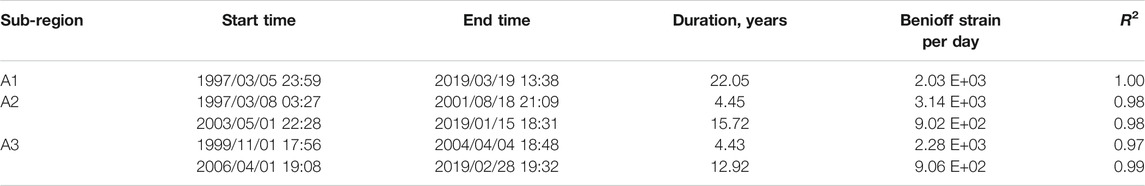
TABLE 4. The cumulative Benioff strain release Ʃ(t) function linear fit intervals for three FVG sub-regions.

One can see that a stable rate of Ʃ–value over the observed time interval is obtained when no large event occurs (A1 sub-region), while in case of a relatively large event, the rate before and after it displays essential differences. Specifically, the M4.9 Sernio earthquake (2002/02/14; Lat: 46.426°N Lon: 13.100°E) eventually marks the separation between the two linear seismic rate intervals for A2 sub-region; the ratio of the Ʃ(t) slope coefficients is 3.5 for A2 two intervals. In a similar way, the 2004 Kobarid event separates two linear seismic rate intervals for A3 sub-region; the ratio of the Ʃ(t) slope coefficients is 2.5 for A3 two time intervals.

Given that Ʃ(t) function within sub-region A1 is characterized by a uniform trend during the whole investigated time span, we compare its slope coefficient with those of the other two regions, A2 and A3, for the different time intervals. Specifically, the ratios of A1 slope coefficient vs. slope A2 and A3 in advance of large events are 1.6 and 1.1, respectively, while after the large events they are both equal to 0.45 (i.e. the slope in A2 and A3 is 2.2 times lower than the slope in A1). Thus, after the large events, the increase of seismic rates in A2 and A3 sub-regions slows down, compared to the steady seismic rate in A1 sub-region.

In this analysis, the slope of Ʃ(t) linear fits essentially characterize the long-term steady trend of seismicity within each area, excluding pre-shock and aftershock related changes. Following Vallianatos and Chatzopoulos (2018), the generalized Benioff strain evolution (which here corresponds to the well-known cumulative Benioff strain, with exponent = 1/2), during the initial part of a main shock preparation process is linear; then, as the time of the earthquake approaches, it deviates from linearity due to the beginning of an accelerating deformation stage. Our analysis shows that the slope of the linear part of cumulative Benioff strain release in areas A2 and A3 changes significantly after the occurrence of the largest earthquakes. According to a non-extensive statistical physics view (Vallianatos and Chatzopoulos, 2018), this observation suggests that the common exponent m associated with the steady (normal) time variation of the generalized Benioff strain within an area, may change after large events.

Unified Scaling Law for Earthquakes Coefficients Space-Time Variability

The available OGS catalog data allowed us to obtain 150 reliable estimates of the medium-term (24.2 years) USLE parameters. Specifically, we considered the hierarchy of square boxes, with linear size equal to 1/2°, 1/4°, 1/8°, 1/16° and 1/32°, respectively, centered at the nodes of a regular grid with 1/16° spacing, which include at least eight earthquakes from the OGS catalog in their 1/16° × 1/16° vicinity. The obtained A, B, and C coefficients are mapped in Figure 5, along with the squared sum of their standard errors σ_A, σ_B, and σ_C. The error of determination of the USLE coefficients does not exceed 0.05, which confirms a rather high quality of the mapped values for the FVG territory. Specifically, there are 58 cells located within sub-region A1, 40 cells within sub-region A2, and 52 cells within A3, while 10 cells are out of three selected sub-regions (Table 1).

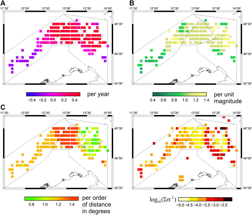
FIGURE 5. The regional maps of A, B, and C coefficients (top panels) and spatial distribution of the sum of standard errors $\sum {\sigma }^2={\sigma }_A^2+{\sigma }_B^2+{\sigma }_C^2$. Color code symbols correspond to estimates associated with cells of size 1/16° × 1/16°.

The seismic activity distribution (coefficient A), normalized to recurrence of a magnitude 3.5 earthquake, in a unit area of 1 ° × 1 ° and in a unit time of one year, varies mainly in the interval [−0.25; 0.45] for A1 sub-region, [0.22; 0.42] for A2 sub-region, and [−0.10; 0.45] for A3 sub-region, with median values 0.10, 0.36 and 0.33 for A1, A2 and A3, respectively. The B values, which characterize the slope of the frequency–magnitude graph, for A1 sub-region vary from 0.8 to 1.2, without any dominant value. For A2 sub-region B-values are well focused: they are equal to 1.1 in 45% cases, and to 1.2 in 55% cases. Within A3 sub-region B-values spread from 0.9 to 1.3.

The fractal dimension of spatial distribution of epicentres C in A1 sub-region has a sharp peak (55% of cells) around the value C = 1.19; within A2 sub-region C varies from 0.90 to 1.47 (50% of cells), with the median value 1.40; in the A3 sub-region C displays a large variability, from below 0.9 to above 1.25.

Figure 6A compares the empirical cumulative distributions functions F_i(coef) of A, B and C coefficients, estimated over the fine scale grid for the three FVG sub-regions. Figure 6B shows the plots of the pairwise difference curves F_m(coef) − F_n(coef) for each USLE coefficient, and allows better understanding the differences in seismic activity in the three sub-regions. For instance, we may observe the remarkable differences between the distributions of C parameter obtained for A1, A2 and A3 sub-regions. Specifically the C-value distributions for A1 corresponds to a (fault) zone with a common dominant Alpine trend, while in A3 it corresponds to linear set of clusters, aligned with a Dinaric trend; finally it characterizes A2 as a highly complex, fractured (fault) zone, located at the Junction of the Alpine and Dinaric (fault) systems.

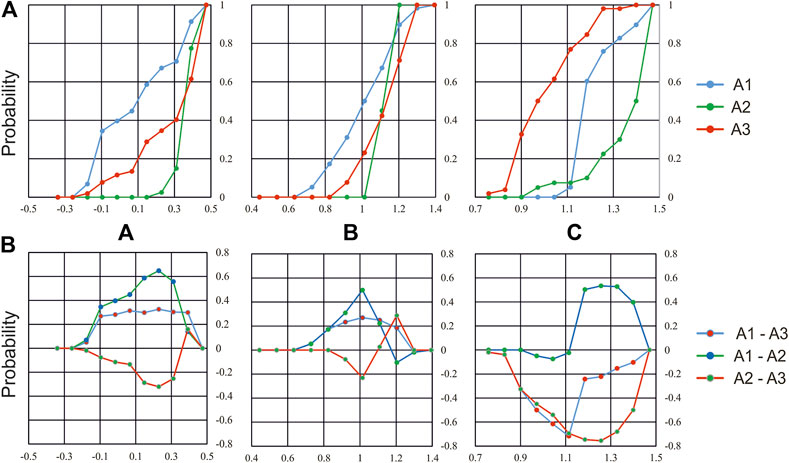
FIGURE 6. Distribution of the USLE coefficients A, B and C, estimated for the fine scale grid in the three sub-regions A1, A2, A3: (A) the cumulative empirical probability functions F_i; (B) the pairwise differences F_m (coef) and F_n (coef), coef = A, B, C.

The maximum absolute difference between the empirical distributions is commonly used in the Kolmogorov–Smirnov two-sample criterion to distinguish whether or not the values from the two samples are drawn from the same statistical distribution of independent variables. Here the two sample Kolmogorov–Smirnov statistic (Smirnov, 1948) λ_K−S is applied to pairwise sets of USLE coefficients distributions, as estimated for each of the different FVG sub-regions. λ_K−S is defined as: λ_K−S (D, n, m) = [n × m/(n + m)]^1/2 × D, where D = max |F_m(coef) − F_n(coef)| is the maximum value of the absolute difference between the empirical distributions F_m(coef) and F_n(coef), coef = A, B, C, whose sample sizes are n and m respectively. Table 5 summarizes the results of comparison for each pairwise set of coefficients, in terms of D and λ_K−S. It is possible to observe that, with 95% probability, the three sub-regions are different in terms of USLE coefficients. The λ_K−S statistic for F(A) allows us to conclude that the distributions of coefficient A for A1 and A2 sub-regions, as well as those for A1 and A3 sub-regions, are significantly different, with probability larger than 99.9%, The A coefficient distributions for A2 vs. A3 can also be marked as different, with probability larger than 95%. The pairwise comparison with λ_K−S statistic for F(B) distributions provides similar results. Specifically the F(B) distributions difference for A1 vs. A2, A1 vs. A3 and A2 vs. A3 confirm that they are all significantly different, with more than 99.9% probability for A1 vs. A2, and 95% probability for the others. For the C-coefficient distributions, the two samples statistics for three pairwise differences allows us rejecting the assumption that coefficients follow the same statistical distribution with more than 99.999% probability.

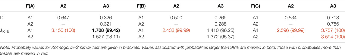
TABLE 5. The Kolmogorov-Smirnov two-sample statistic λ_K−S applied to F(coef), the Sample size are in Table 1.

Besides the medium-term average estimates described so far, the time-variable estimates of USLE coefficients have been performed for the fine grid, considering moving six-years time intervals with one year shift. As a results 19 sets (with ending time from 2001 to 2019 years) of A, B and C coefficients values have been obtained for each of the A1, A2 and A3 sub-regions. It is worth noting that, for each six-years times interval (namely 1995/01/01–2001/01/01, … , 2014/01/01–2019/01/01), the number of cells with reliable data for SCE algorithm calculation may be different, which may influence the reliability of coefficients estimation.

The analysis of the pairwise 2D correlation plots of the A-values, B-values and C-values, computed for each six-years time interval (see Supplementary Material S3), allows us to observe that the coefficients and their correlation change significantly over time, in all of the three considered sub-regions (Supplementary Figures S3.1–S3.3). To facilitate the analysis of such variations, three time periods have been considered: 1) four time windows (six-years long, with ending time from 2001 to 2004), where USLE parameters are apparently affected by 1998/04/12 M = 5.6 Kobarid earthquake and related aftershocks; 2) six time windows (six-years long, with ending time from 2005 to 2010), with USLE parameters apparently affected by the 2004/07/12 M = 5.1 Kobarid earthquake aftershocks; 3) nine time windows (six-years long, with ending time from 2011 to 2019) without any principal (M ≥ 5.0) earthquake, and thus providing presumably independent (background) USLE parameters values. The A-values display relatively stable values in all three FVG sub-regions, except for the high variability of A-values within A3 sub-region starting from 2011. During the period from 2011 to 2019 the B-values decrease progressively in each of the three FVG sub-regions (Supplementary Figures S3.1c,S3.3c), while the A-value slightly increases in sub-region A1. Accordingly, the number of low magnitude earthquakes decreases during the 2011–2019 all over the FVG territory, in A3 sub-region especially. C-values in the three sub-regions vary from one to less than 1.4 and, from 2000 to 2010 years, take relatively low values in A2 and A3 sub-regions due to the aftershocks effect; in addition, an interesting decreasing trend of C-values, down to 0.8, characterizes the A1 region from 2013 to 2019 years.

Finally, to investigate in more detail the space-time variations of USLE coefficients, the medians of A-values, B-values and C-values have been computed, for six-years time intervals with shift of one year, within each of nine out of 10 seismic districts of Friuli-Venezia Giulia Region (Supplementary Figure S1), as defined by Bressan et al. (2018; 2019). The PL and FOA districts are not considered, because they do not include enough events for reliable estimation of USLE parameters. The values of the medians obtained for each of the nine seismic districts (Supplementary Figure S3.4) support the grouping into the three sub-regions used in this study: the districts that compose A3 sub-region (TAR, BA, BOV) display temporal trends of the A-B- and C-values much different that the other districts.

Control Parameter η Temporal Variability

The main parameter, which allows characterizing the seismic rate in terms of USLE, is the control parameter η defined in Eq. 2. In order to compute the η-values, necessary to investigate the temporal variability of this parameter within A1, A2 and A3 sub-regions, we used the global values of USLE coefficients listed in Table 1. Accordingly, the A, B and C coefficients used in Eq. 2 correspond to long-term robust estimates of USLE, which account for the moderate-large M > 4.0 earthquakes that are reported in USGS Global Hypocenter Data base system, 1964–2001, (Nekrasova and Kossobokov, 2019). Note that for the purpose of this analysis we have extended the time window, including an additional time interval from 1988 to 1994, so as to be able and analyze seismicity changes before the principal 1998 Kobarid earthquake; according to Peruzza et al. (2015) this time interval is characterized by uniform OGS network conditions, and thus can be used for our analysis.

Figure 7 shows the plots of the 50-events moving average of 〈η〉 vs. origin time, for the earthquakes located within the A1, A2 and A3 sub-regions, which occurred during the time interval from January 1988 to April 2019. It is possible to observe some nearly-flat portions of the graphs, where the moving averages vary within one decimal order; these periods of stability are characterized by a low rate of seismicity. To quantify this feature, let us define the periods of stability by the condition that {t: 〈η〉(t) is larger than 〈η〉_max/10}, where 〈η〉_max is the maximal value of 〈η〉 over the entire considered time interval. Table 6 lists the periods of 〈η〉 stability identified for the three FVG sub-regions. For the A3 sub-region we identified three periods of stability of 〈η〉 interrupted by bursts of activity, associated with the origin times of principal earthquakes and their aftershocks. Namely, before the Kobarid April 12, 1998 event, a 5.8 years time interval with very low seismic rate 〈η〉 = 10.02 ± 0.39 is detected from 1992/07/13 to 1998/04/12; between the two principal events, precisely from 2001/10/26 to 2004/07/13, a 2.8 years interval with much larger seismic rate 〈η〉 = 3.59 ± 0.11 has been identified; during the last 13.4 years interval, from 2005/10/02 to the end of the OGS catalog, an intermediate level seismic rate, with 〈η〉 = 6.92 ± 0.20, is quantified. For A1 sub-region we determined four periods of 〈η〉 stability: a low seismic rate interval with 〈η〉 = 7.87 ± 0.49 in 1990/09/03–1996/06/29; two comparatively higher rate intervals in 1998/02/07–2000/09/19 and 2001/03/18–2003/12/27, with 〈η〉 equal 2.71 ± 0.05 and 3.31 ± 0.11 respectively; a 15 years interval of moderate seismic rate, with 〈η〉 value 4.71 ± 0.08, from 2004/03/24 to the end of catalog. Finally, according to η control parameter, a single 〈η〉 stable interval can be identified for A2 sub-region, from 1988/09/18 to 2019/01/15 (30.3 years), with 〈η〉 value 2.51 ± 0.05, which apparently characterizes the relatively high and constant seismic rate of this area.

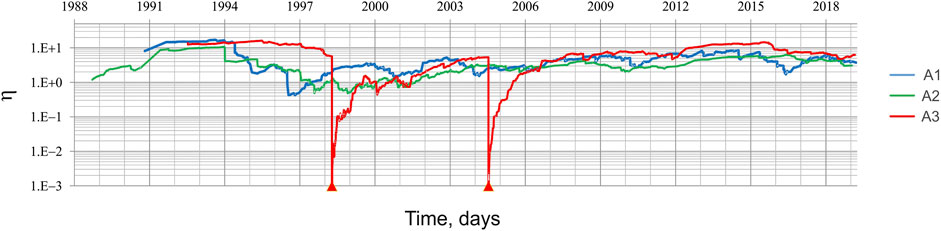
FIGURE 7. USLE control parameter η (1988–2019) moving average per 50 events in three FVG sub-regions vs. earthquake origin time (A1 – blue line, A2-green line, A3 – red line). Note: the origin times of the two principal earthquakes (Table 2) are marked with red triangles on the origin time scale.

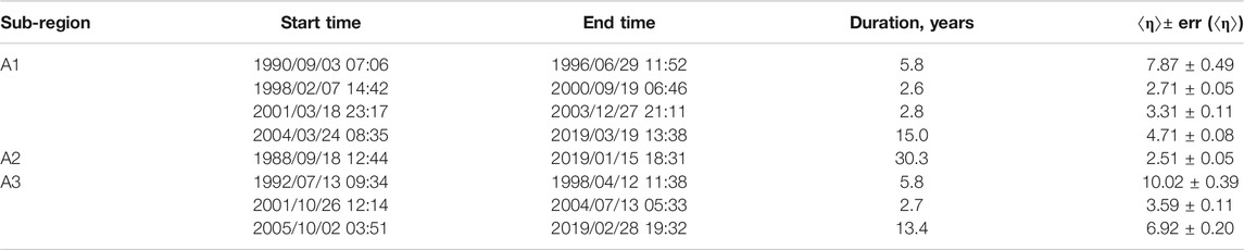
TABLE 6. Periods of stability of the USLE control parameter 〈η〉 for three Friuli-Venezia Giulia sub-regions.

The discrete and cumulative empirical distribution functions of η for each of three sub-regions are compared (left top panel, Figure 8 and central top panel, Figure 8), confirming a broad spread over about six or more decimal orders of the bulk density distribution of η. According to the nonparametric two-sample Kolmogorov–Smirnov statistic λ_K-S, applied to the pairwise differences of η distribution functions η(A3), η(A2) and η(A3) for the three sub-regions, all of them have different probability distribution, with probability above 99% (Tabure 7). Finally, the comparison is restricted to the most recent time interval, from 2005/10/02 to the end of OGS catalog, when according to Table 6, stable intervals of 〈η〉 are obtained in all FVG sub-regions (Figure 8, bottom panels). The pairwise differences of η distribution functions for 2005–2019 time interval (Figure 8, right bottom panel) and the λ_K-S values for pairwise differences of η distributions (Tab. 7), confirm that even for the time period without principal earthquakes η(A3), η(A2) and η(A3) do not come from the same distribution, with probability above 99% in almost all cases (except for η(A2) vs. η(A3), for which probability is still above 95%).

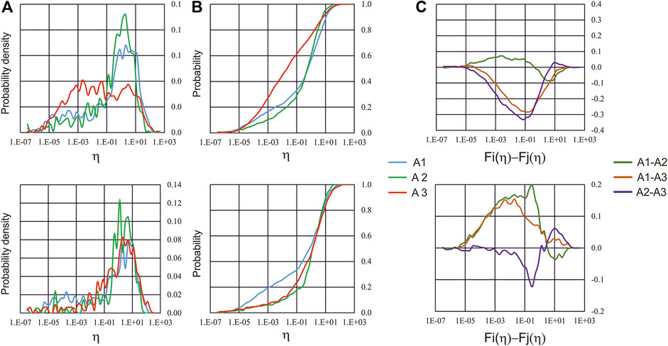
FIGURE 8. Empirical density (A) and cumulative (B) distribution functions of USLE control parameter η and (C) pairwise difference F_i(η) − F_j(η) for A1, A2 and A3 FVG sub-regions in 1988–2019 time interval (top panels) and in 2005/10/2–2019 time interval (bottom panels).

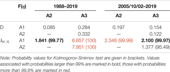
TABLE 7. The Kolmogorov-Smirnov two-sample statistic λ_K−S applied to distribution functions of USLE control parameter η.

Discussion and Conclusions

In order to get new insights in the evolving dynamics of seismicity, which controls its temporal variations within different areas of FVG territory, a multi-parametric analysis was performed. Different parameters, including inter-event times τ, Benioff strain release Ʃ, and the control parameter η of the USLE, were used to assess heterogeneity in spatial and temporal patterns of earthquakes occurrence, as reported in OGS catalog for Northeastern Italy and its surroundings.

As a preliminary step, the space variability of the USLE coefficients, namely the seismicity rate (A), the earthquake magnitude exponent (B), and the fractal dimension of epicenter loci (C), was examined in some detail, comparing the values obtained within three sub-regions defined grouping seismic districts with similar tectonic features (Bressan et al., 2019). Different tectonic domains, in fact, can be identified within the study region, which is located at the junction between the E-W oriented Alpine and the NW-SE oriented Dinaric fault systems (Figure 1A). According to Bressan et al. (2018), the superposition of different tectonic phases caused high fragmentation and heterogeneity of the upper crust in this area, which is characterized by sharp lateral heterogeneities of the elastic moduli in the upper crustal structure (down to 10 km depth). The analysis performed in this study confirms that the features of seismic energy release, including their temporal variations, are statistically different within the three outlined sub-regions A1, A2 and A3. The spatial distribution of USLE coefficients is shown in Figure 5, while their empirical probability functions are given in Figure 6. Specifically, the coefficient of magnitude balance B, which is analogous to the b-value of the Gutenberg-Richter law and quantifies the relative proportion between small and large earthquakes, is characterized by well focused B values within [1.1–1.2], in the central zone (area A2); this area hosted the M6.4 1976 Friuli earthquake, but since then instrumental seismicity has been characterized only by moderate size events. At the same time, the western zone (area A1), corresponding to the Carnie Pre-Alps, is characterized by higher variability, which indicates higher spatial heterogeneity in the seismic energy release, and by low-intermediate B values, within the range [0.8–1.2], and thus by a comparatively low ratio of small-moderate magnitude events. Instead, the Dinaric eastern zone (area A3) is associated with relatively higher B values, in the range [0.9–1.3], evidencing the occurrence of a comparatively large number small to moderate seismic events, mostly related with aftershocks occurrence. Significant differences have been observed between the distributions of the fractal dimension of earthquake epicenters C (Figure 5), obtained for A1, A2 and A3 sub-regions (Figure 1A). Specifically, within area A3, C appears characterized by quite low values, mostly up to 1.0, which can be related with a linear set of clusters, aligned with a Dinaric trend. This is possibly due to the occurrence, within area A3 of the two largest magnitude events reported in the considered data set (the 1998 and 2004 Kobarid earthquakes) that, along with their highly clustered aftershocks, dominate seismicity in the area. The western area (area A1) displays prevailing intermediate values, corresponding to a (fault) zone with a common dominant Alpine trend and associated with rather complex swarm-like earthquake sequences (Peresan and Gentili, 2018). Finally, the central zone (area A2) is characterized by higher fractal values, corresponding to a highly complex, fractured (fault) zone, located at the junction of the Alpine and Dinaric (fault) systems (Figure 1A).

In the long-term of the considered dataset (i.e., from 1988 to 2019) we found different intervals of rather steady seismic activity, which are characterized by a near constant value of η, with switches at times of transition associated with the relatively large M_d > 5.0 events. As long as the temporal features of seismicity are concerned, a time interval of rather stable seismic activity could be determined according to the different parameters; during such interval, starting on 2005 and up 2019 (i.e., up to the end of available data) no major earthquakes (i.e., M_d > 5.0) are reported in the catalog, thus providing presumably independent (background) parameters values. Although the temporal pattern of activity rate changes identified in this study reflects trends at the sub-regions scale, this result appears compatible with the observation of a period of rather low background seismicity rate (i.e. for the declustered catalog) ongoing since more than a decade, detected by Benali et al. (2020) for the whole FVG region.

The results obtained for Northeastern Italy and surrounding areas confirm similar analysis performed on a global scale, in advance and after the largest earthquakes worldwide. Specifically, we found that: 1) the dynamical changes of τ, Ʃ, and η in the three sub-regions highlight a number of different seismic regimes; 2) the seismic activity prior and after the occurrence of strong main shocks (e.g., the 1998 and 2004 Kobarid earthquakes) is characterized by significantly different parameters within the related sub-region; 3) the USLE coefficients in FVG region are time-dependent (as observed in Nekrasova and Kossobokov, 2005; Nekrasova, 2007; Nekrasova et al., 2011) and show up correlated, displaying interesting features in dynamics of seismicity that can be related with major earthquakes (see Supplementary Figures S3.1–S3.3).

The temporal changes of the USLE coefficients estimated for three FVG sub-regions exposed correlated, though complex behaviors in dynamics of the Earth crust hierarchical system of blocks-and-faults. In addition, the analysis of time variations of the cumulative Benioff strain release, Ʃ(t), evidenced that the slope of its linear long-term trend may change significantly after the occurrence of a major earthquake. Although the number of the moderate earthquakes in the FVG region is too small for contributing to “the hypothesis that many large earthquakes are preceded by accelerating-decelerating seismic release rates which are described by a power law time to failure relation” (Vallianatos and Chatzopoulos, 2018), according to a non-extensive statistical physics view, our observations suggest that the steady (normal) state of the system (as described by the common exponent m associated with the time variation of the Benioff strain within an area), may change after the occurrence of a large earthquake.

The obtained results highlight non-stationarity of seismic activity, at a time-scale of several years and up to decades, in agreement with earlier findings by Benali et al. (2020), an element that should be taken into account for improving local seismic hazard assessment. The regions and time intervals identified in this study, which display homogeneous features of seismic activity, may supply valuable information toward time-dependent seismic hazard assessment (e.g., Kossobokov et al., 2015 and references therein), while providing new constraints for earthquakes forecasting in Northeastern Italy.

Data Availability Statement

Publicly available datasets were analyzed in this study. The earthquake datasets used in this study are published as yearly and monthly bulletins by the National Institute of Oceanography and Applied Geophysics (OGS) and are publicly available via the OGS website (http://www.crs.inogs.it/bollettino/RSFVG/).

Author Contributions

AN performed time series computations, and ABC coefficients analysis, while AP provided the data, performed preliminary data analysis and defined the setting and regions for investigation. Both AN and AP collaborated at data interpretation and manuscript write up.

Funding

The IEPT RAS researcher part of this study is supported by grant of the Russian Science Foundation (project No. 20–17–00180). The research also benefited from financial support by Protezione Civile della Regione Autonoma Friuli-Venezia Giulia (Italy) in the framework of the cooperation with OGS (“Collaborazione nell'ambito del monitoraggio sismico e meteomarino di interesse Regionale e per il supporto tecnico-scientifico nella prevenzione e gestione di emergenze sismiche, meteomarine e ambientali sul territorio e lungo le coste della Regione Friuli Venezia Giulia”).

Conflict of Interest

The authors declare that the research was conducted in the absence of any commercial or financial relationships that could be construed as a potential conflict of interest.

Acknowledgments

The authors are grateful to V. G. Kossobokov (IEPT RAS) for valuable comments and to C. Barnaba (OGS) for useful discussions. Earthquake data used in this study are published by the National Institute of Oceanography and Applied Geophysics (OGS) and are publicly available at www.crs.inogs.it/bollettino/RSFVG/. The data are collected in the framework of the cooperation between OGS and Regione Autonoma Friuli Venezia Giulia Civil Protection.

Supplementary Material

The Supplementary Material for this article can be found online at: https://www.frontiersin.org/articles/10.3389/feart.2020.590724/full#supplementary-material.

References

Bak, P., Christensen, K., Danon, L., and Scanlon, T. (2002). Unified scaling law for earthquakes. Phys. Rev. Lett. 88, 178501–178504. doi:10.1103/PhysRevLett.88.178501
Benali, A., Peresan, A., Varini, E., and Talbi, A. (2020). Modelling background seismicity components identified by nearest neighbour and stochastic declustering approaches: the case of Northeastern Italy. Stoch. Environ. Res. Risk Assess. 34 (6), 775–791
Benioff, H. (1951). Global strain accumulation and release as related by great earthquakes. Bull. Geol. Soc. Am. 62, 331–338.
Bressan, G., Barnaba, C., Bragato, P. L., Peresan, A., Rossi, G., and Urban, S. (2019). Distretti sismici del Friuli Venezia Giulia, Bollettino di Geofisica Teorica. Applicata 60, S1–S74. doi:10.4430/bgta0300
Bressan, G., Barnaba, C., Bragato, P., Ponton, M., and Restivo, A. (2018). Revised seismotectonic model of NE Italy and W Slovenia based on focal mechanism inversion. J. Seismol. 22 (6), 1563–1578. doi:10.1007/s10950-018-9785-2
Chochlaki, K., Vallianatos, F., and Michas, G. (2018). Global regionalized seismicity in view of non-extensive statistical physics. Phys. Stat. Mech. Appl. 493, 276–285. doi:10.1016/j.physa.2017.10.020
Christensen, K., Danon, L., Scanlon, T., and Bak, P. (2002). Unified scaling law for earthquakes. Proc. Natl. Acad. Sci. U.S.A. 99 (Suppl. 1), 2509–2513. doi:10.1073/pnas.012581099
Gorshkov, A., Panza, G. F., SolovievAoudia, A. A., and Peresan, A. (2009). Delineation of the geometry of nodes in the Alps-Dinarides hinge zone and recognition of seismogenic nodes (M ≥ 6). Terra. Nova. 21 (4), 257–264. doi:10.1111/j.1365-3121.2009.00879.x
Gutenberg, R., and Richter, C. F. (1944). Frequency of earthquakes in California. Bull. Seismol. Soc. Am. 34, 185–188.
Kossobokov, V. G., and Mazhkenov, S. A. (1989). “On similarity in the spatial distribution of seismicity,” in Computational seismology and geodynamics. Editor D. K. Chowdhury (Washington DC: AGU), 1, 6–15.
Kossobokov, V. G., and Mazhkenov, S. A. (1988). “Spatial characteristics of similarity for earthquake sequences: fractality of seismicity,” in Lecture notes of the workshop on global geophysical informatics with applications to research in earthquake prediction and reduction of seismic risk [15 Nov–16 Dec., 1988]. Trieste: ICTP, 15.
Kossobokov, V. G., and Nekrasova, A. K. (2019). Aftershock sequences of the recent major earthquakes in New Zealand. Pure Appl. Geophys. 176, 1–23. doi:10.1007/s00024-018-2071-y
Kossobokov, V. G., and Nekrasova, A. K. (2017). Characterizing aftershock sequences of the recent strong earthquakes in Central Italy (2017). Pure Appl. Geophys. 174 (10), 3713–3723. doi:10.1007/s00024-017-1624-9
Kossobokov, V. G., Peresan, A., and Panza, G. F. (2015). On operational earthquake forecast and prediction problems. Seismol Res. Lett. 86 (2A), 287–290. doi:10.1785/0220140202
Kossobokov, V. (2020). “Unified scaling law for earthquakes that generalizes the fundamental Gutenberg-Richter relationship,” in Encyclopedia of solid Earth Geophysics, encyclopedia of Earth sciences series. 2nd Edition. Editor H. K. Gupta doi:10.1007/978-3-030-10475-7_257-1/Ed.H
Mignan, A., and Woessner, J. (2012). Estimating the magnitude of completeness in earthquake catalogs, community online resource for statistical seismicity analysis. Available at: http://www.corssa.org (Accessed October 20, 2020). doi:10.5078/corssa-00180805
Nekrasova, A. (2007). “Part 4: earthquake Hazard in the Alps - 4.1 - unified scaling law for earthquakes in the Alps: a multiscale application,” in Final report of the ALPS-GPSQuakenet project, Interreg III B Alpine Space programme. Muenchen: Bayerische akademie der Wissenschaften. 63–85.
Nekrasova, A. K., and Kossobokov, V. G. (2019). Unified scaling law for earthquakes: global map of parameters. ISC Seismolog. Dataset Rep. doi:10.31905/XT753V44
Nekrasova, A., and Kossobokov, V. (2003). Generalized Gutenberg-Richter recurrence law: global map of parameters. Geophys. Res. Abst. 5.Abstract EAE03-A-03801.
Nekrasova, A., and Kossobokov, V. (2002). Generalizing the Gutenberg-Richter scaling law. EOS Trans. AGU. 83 (47). Fall Meet. Suppl., Abstract NG62B-0958.
Nekrasova, A., Kossobokov, V., Parvez, I. A., and Tao, X. (2015). Seismic hazard and risk assessment based on the unified scaling law for earthquakes. Acta Geod. Geophys. 50 (1), 21–37. doi:10.1007/s40328-014-0082-4
Nekrasova, A., Kossobokov, V., Peresan, A., Aoudia, A., and Panza, G. F. (2011). A multiscale Application of the unified scaling law for earthquakes in the central mediterranean area and alpine region. Pure Appl. Geophy. 168 (1–2). doi:10.1007/s00024-010-0163-4
Nekrasova, A., and Kossobokov, V. (2005). Temporal variation of the coefficients of Unified scaling law for earthquakes on the east of Honshu Island (Japan). Dokl. Earth Sci. 405A (No. 9), 1352–1355.
Nekrasova, A., Peresan, A., Magrin, A., and Kossobokov, V. (2016). The unified scaling law for earthquakes in the Friuli -Venezia Giulia region. Geophys. Res. Abstr. 18, EGU2016–17706.
OGS (2019). OGS Bulletin, Centro di Ricerche Sismologiche (CRS), Istituto Nazionale di Oceanografia e di Geofisica Sperimentale (OGS), Udine, Italy. Available at: http://www.crs.inogs.it (Accessed May 30, 2019).
Parvez, I. A., Nekrasova, A., and Kossobokov, V. (2014). Estimation of seismic hazard and risks for the Himalayas and surrounding regions based on Unified Scaling Law for Earthquakes. Nat. Hazards. 71 (1), 549–562. doi:10.1007/s11069-0130926-1
Peresan, A., and Gentili, S. (2020). Identification and characterization of earthquake clusters: a comparative analysis for selected sequences in Italy and adjacent regions. Boll. Geof. Teor. Appl. 61 (1), 57–80. doi:10.4430/bgta0249
Peresan, A., and Gentili, S. (2018). Seismic clusters analysis in Northeastern Italy by the nearest-neighbor approach. PEPI 274, 87–104. doi:10.1016/j.pepi.2017.11.007
Peruzza, L., Garbin, M., Snidarcig, A., Sugan, M., Urban, S., Renner, G., et al. (2015). Quarry blasts, underwater explosions and other dubious seismic events in NE Italy from 1977 till 2013. Boll. Geof. Teor. Appl. 56 (4), 437–459.
Slejko, D., Neri, G., Orozova, I., Renner, G., and Wyss, M. (1999). Stress field in Friuli (NE Italy) from fault plane solutions of activity following the 1976 main shock. Bull. Seism. Soc. Am. 89, 1037–1052.
Smirnov, N. (1948). Table for estimating the goodness of fit of empirical distributions. Ann. Math. Stat. 19, 279–281. doi:10.1214/aoms/1177730256
Tsallis, C. (1988). Possible generalization of Boltzmann–Gibbs statistics. J. Stat. Phys. 52, 479–487. doi:10.1007/BF01016429
Vallianatos, F., and Chatzopoulos, G. (2018). A complexity view into the physics of the accelerating seismic release hypothesis: theoretical principles. Entropy 20 (10), 754. doi:10.3390/e20100754
Keywords: earthquake sequences, unified scaling law for earthquakes, seismic dynamics, control parameter, Benioff strain release, seismic hazard assessment, earthquake forecast/prediction
Citation: Nekrasova A and Peresan A (2021) Unified Scaling Law for Earthquakes: Space-Time Dependent Assessment in Friuli-Venezia Giulia Region. Front. Earth Sci. 8:590724. doi: 10.3389/feart.2020.590724
Received: 02 August 2020; Accepted: 17 November 2020;
Published: 08 January 2021.
Edited by:
Joanna Faure Walker, University College London, United KingdomReviewed by:
Filippos Vallianatos, Technological Educational Institute of Crete, GreeceR/ B. S. Yadav, Kurukshetra University, India
Copyright © 2021 Nekrasova and Peresan. This is an open-access article distributed under the terms of the Creative Commons Attribution License (CC BY). The use, distribution or reproduction in other forums is permitted, provided the original author(s) and the copyright owner(s) are credited and that the original publication in this journal is cited, in accordance with accepted academic practice. No use, distribution or reproduction is permitted which does not comply with these terms.
*Correspondence: Anastasia Nekrasova, nastia@mitp.ru