Uncertainties in Projections of the Baltic Sea Ecosystem Driven by an Ensemble of Global Climate Models
 Sofia Saraiva1,2
  H. E. Markus Meier1,3*
  Helén Andersson1
  Anders Höglund1
  Christian Dieterich1
  Matthias Gröger1
  Robinson Hordoir1,4,5
  Kari Eilola1
- 1Swedish Meteorological and Hydrological Institute, Norrköping, Sweden
- 2MARETEC, Instituto Superior Técnico, University of Lisbon, Lisbon, Portugal
- 3Department of Physical Oceanography and Instrumentation, Leibniz Institute for Baltic Sea Research Warnemünde, Rostock, Germany
- 4Institute of Marine Research, Bergen, Norway
- 5Bjerknes Centre for Climate Research, Bergen, Norway
Many coastal seas worldwide are affected by human impacts such as eutrophication causing, inter alia, oxygen depletion, and extensive areas of hypoxia. Depending on the region, global warming may reinforce these environmental changes by reducing air-sea oxygen fluxes, intensifying internal nutrient cycling, and increasing river-borne nutrient loads. The development of appropriate management plans to effectively protect the marine environment requires projections of future marine ecosystem states. However, projections with regional climate models commonly suffer from shortcomings in the driving global General Circulation Models (GCMs). The differing sensitivities of GCMs to increased greenhouse gas concentrations affect regional projections considerably. In this study, we focused on one of the most threatened coastal seas, the Baltic Sea, and estimated uncertainties in projections due to climate model deficiencies and due to unknown future greenhouse gas concentration, nutrient load and sea level rise scenarios. To address the latter, simulations of the period 1975–2098 were performed using the initial conditions from an earlier reconstruction with the same Baltic Sea model (starting in 1850). To estimate the impacts of climate model uncertainties, dynamical downscaling experiments with four driving global models were carried out for two greenhouse gas concentration scenarios and for three nutrient load scenarios, covering the plausible range between low and high loads. The results suggest that changes in nutrient supply, in particular phosphorus, control the long-term (centennial) response of eutrophication, biogeochemical fluxes and oxygen conditions in the deep water. The analysis of simulated primary production, nitrogen fixation, and hypoxic areas shows that uncertainties caused by the various nutrient load scenarios are greater than the uncertainties due to climate model uncertainties and future greenhouse gas concentrations. In all scenario simulations, a proposed nutrient load abatement strategy, i.e., the Baltic Sea Action Plan, will lead to a significant improvement in the overall environmental state. However, the projections cannot provide detailed information on the timing and the reductions of future hypoxic areas, due to uncertainties in salinity projections caused by uncertainties in projections of the regional water cycle and of the mean sea level outside the model domain.
Introduction
Regional projections of future climate based on dynamical downscaling of global model results using regional climate models (RCMs) suffer from considerable uncertainties caused by (1) shortcomings of global and regional climate models, (2) unknown future greenhouse gas concentrations, (3) natural variability, and (4) experimental design (e.g., Hawkins and Sutton, 2009; Kjellström et al., 2011; Déqué et al., 2012; Mathis et al., 2018). Global climate models are based on General Circulation Models (GCMs) or even Earth System Models (ESMs) and are useful tools to address climate variability on the global scale (acronyms are explained in Table 1). However, they have still significant shortcomings on regional scales, inter alia, because their horizontal grids are too coarse to resolve details of the orography and the land-sea mask, which might be important to the regional climate (Stocker et al., 2013). To overcome the limitations of global climate models for regional climate studies, limited-area RCMs with high resolution were developed for the region of interest, driven by data from GCMs or ESMs at the lateral boundaries of the model domain (e.g., Giorgi and Mearns, 1991). With such an experimental setup, scenario simulations were carried out, with the aim to study the impact of climate change and to develop climate adaptation strategies for selected regions (e.g., Räisänen et al., 2004).
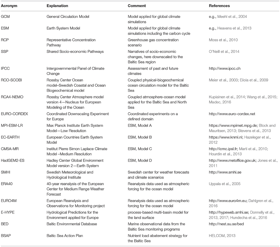
Table 1. List of acronyms.
As mentioned above, these regional projections have limitations. For instance, Christensen et al. (2010) and Jacob et al. (2014) studied the uncertainties in regional atmospheric projections, whereas systematic analyses of uncertainties in regional ocean projections have not been performed yet. For marine ecosystems, another source of uncertainty has to be considered (in addition to the sources mentioned above). As the socioeconomic development in the catchment area of the coastal sea is unknown, future nutrient loads from land and atmospheric depositions of nitrogen and phosphorus are speculative, contributing to the uncertainties of the projections of the marine ecosystems (e.g., Meier et al., 2011a).
In this study, we focus on the Baltic Sea (Figure 1), which is a semi-enclosed coastal sea with a large catchment area located in northern Europe (Sjöberg, 1992). The Baltic Sea region is divided into two sub-regions. Extensive forests, low population density, mostly rocky coasts and subarctic winter climate characterize the north. On the other hand, the south is characterized by agricultural land, high population density, mostly sandy coasts, and a moderate winter climate. Approximately 90 million people live in the catchment area of the Baltic Sea, creating a considerable impact on the marine environment (Ahtiainen and Öhman, 2014). Reinforced river-borne nutrient loads from agriculture and sewage treatment plants since the 1940/50s caused the world largest anthropogenic-induced hypoxic bottoms (Conley et al., 2009; Conley, 2012; Gustafsson et al., 2012; Carstensen et al., 2014; Meier et al., 2018). In addition to environmental pressures, the Baltic Sea is affected by global warming more than other coastal seas, perhaps because of its proximity to the Arctic, hydrodynamic features and land-locked location (BACC II Author Team, 2015). During 1982-2006, the Baltic Sea has warmed up more than any other large marine ecosystem (Belkin, 2009).
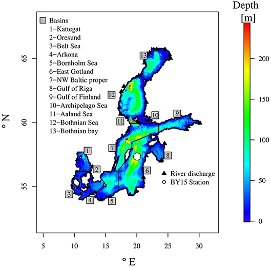
Figure 1. The Baltic Sea: bathymetry, river discharges, and sub-basins as defined in this study. The Baltic proper comprises Arkona, Bornholm, East Gotland and Northwest Gotland basins. In addition, the location of the monitoring station at Gotland Deep (BY15) is shown (white circle).
Since 2000, future projections of the Baltic Sea have been carried out for supporting the design of appropriate management plans to more effectively protect the marine environment. The first projections were made with pure hydrodynamic models (Omstedt et al., 2000; Meier, 2002a, 2006; Döscher and Meier, 2004; Meier et al., 2004) and, later, with coupled physical-biogeochemical models (Meier et al., 2011c). However, these first studies did not address enough on the uncertainties related to future projections.
To estimate uncertainties, mini-ensembles of continuous simulations from the present to the future climate driven by two GCMs and two greenhouse gas emission scenarios were produced (Neumann, 2010; Friedland et al., 2012; Meier et al., 2012a; Ryabchenko et al., 2016). In addition, three different Baltic Sea ecosystem models were used to estimate the uncertainties caused by deficiencies in the representation of marine ecosystem processes (e.g., Meier et al., 2011a, 2012b,c). Omstedt et al. (2012) even used three GCMs and three greenhouse gas emission scenarios, although they applied a regional atmospheric model instead of a regional coupled atmosphere-ocean model for the dynamical downscaling. By using a regional atmosphere model, the projected sea surface temperatures (SSTs) were based on the SSTs from GCMs that do not take the regional details of the Baltic Sea region into account, causing considerable deficiencies in projections (e.g., Meier et al., 2011b). Hence, uncertainties of Baltic Sea projections originating from climate model uncertainties have not been thoroughly assessed. An exception is the study by Meier et al. (2006), who studied the spread of a multi-model ensemble consisting of 16 scenario simulations based on seven regional models, five global models and two greenhouse gas emission scenarios. However, Meier et al. (2006) focused only on salinity thus, not addressing the changes in the biogeochemical cycles. They also neglected changes in variability on time scales longer than 1 year. In all other dynamical downscaling studies of the Baltic Sea, only one or two GCMs were used.
In this study, we focus on uncertainties in Baltic Sea water quality projections caused by uncertainties due to climate model deficiencies and due to unknown greenhouse gas concentration, nutrient load and sea level rise scenarios. According to Hawkins and Sutton (2009), who have found that the uncertainties due to natural variability at the end of the 21st century are small, we have neglected this source of uncertainty. Climate model uncertainties are defined as the spread (variance) in regional projections for the Baltic Sea ecosystem caused by GCM deficiencies inherited to the applied RCM and regional ocean model via the dynamical downscaling approach. These climate model uncertainties are compared with estimated uncertainties due to unknown greenhouse gas concentration, nutrient load, and sea level rise scenarios. For our aim, we investigate variances of an ensemble of scenario simulations and of selected sub-sets of the entire ensemble.
The highly non-linear dynamics of the Baltic Sea ecosystem are controlled by nutrient loads from land and from the atmosphere, water temperature, salinity, light conditions, mixed layer depth, sea-ice conditions (only in the northern Baltic Sea), saltwater water inflows (only in the Baltic proper and the Gulf of Finland, see Figure 1) and resuspension (e.g., Wulff et al., 2001). Hence, all uncertainties in scenario simulations of air temperature, precipitation, wind speed, cloudiness, atmospheric circulation patterns and river runoff will have an impact on projected biogeochemical cycles (BACC II Author Team, 2015). For example, higher water temperatures may increase the production and remineralization of organic material (i.e., may intensify the internal nutrient cycling) and reduce air-sea fluxes of oxygen (Meier et al., 2011a). Further, increased river runoff may reinforce river-borne nutrient loads (Stålnacke et al., 1999; Meier et al., 2012b) and a shallower mixed layer depth may alter phytoplankton blooms (Hieronymus et al., 2018). In the northern Baltic Sea, the shrinking sea-ice cover will lead to an earlier onset and termination of the spring bloom due to improved light conditions (Eilola et al., 2013). The frequency of saltwater inflows may slightly increase due to changes in the large-scale atmospheric circulation patterns (Schimanke et al., 2014). Global mean sea level rise may enhance the salt transport into the Baltic Sea causing increased stratification, reduced deep water ventilation, and expanding hypoxia in the Baltic proper (Meier et al., 2017). As the Baltic Sea is shallow with a mean depth of 52 m only, nutrient exchanges between sediment and water column and resuspension of organic matter are important processes for the biogeochemical cycling (Almroth-Rosell et al., 2011). Eilola et al. (2012) suggested that in future climate the exchange between shallow and deep waters might be intensified and that the internal removal of phosphorus might be weaker. In areas with reduced sea-ice cover, the winter mixing may increase, and the oxygen conditions in lower layers may improve (Eilola et al., 2013). An increase of wave-induced resuspension may cause an increase of nutrient transportation from the productive coastal zone into the deeper areas (Eilola et al., 2013).
The paper is organized as follows. In the next section “Data and Methods,” the regional climate ocean model, the regional coupled atmosphere-ocean model, driving GCMs, greenhouse gas concentration and nutrient load scenarios, and the experimental setup are introduced. In the section “Results,” the results of future projections for temperature, salinity, selected biogeochemical fluxes (primary production and nitrogen fixation) and hypoxic areas are presented. Finally, uncertainties of the projections and the suspected shortcomings of the study are discussed and some conclusions of the study are drawn.
Data and Methods
A series of scenario simulations with a coupled physical-biogeochemical Baltic Sea model (see next section) was performed. The Baltic Sea model was driven by regionalized GCM data using the dynamical downscaling approach (see section on Regional Climate Data Sets). In this approach, the atmospheric forcing data were calculated using a RCM with GCM data at the lateral boundaries. The resulting atmospheric surface fields of 10 m wind, 2 m air temperature, 2 m specific humidity, precipitation, total cloudiness, and sea level pressure were then applied to force the Baltic Sea model and a hydrological/land surface model for the Baltic Sea catchment area. The output variables of the latter model are river runoff and nutrient loads to the Baltic Sea model. As the nutrient loads depend on not only precipitation and air temperature at the land surface, but also on land use, agricultural practices and sewage water treatment, all scenario simulations were performed under different socio-economic scenarios covering a plausible range between low and high loads (see section on Nutrient Load Scenarios). Figure 2 presents a conceptual diagram of the dynamical downscaling approach used in this study. As the global mean sea level rise is not considered in the scenario simulations, two additional sensitivity experiments were performed to estimate the impact of a higher sea level at the lateral boundary of the Baltic Sea model (see section on Experimental Setup).
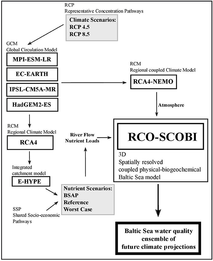
Figure 2. Conceptual diagram of the modeling approach used in the study.
Baltic Sea Model
In this study, a three-dimensional ocean circulation model is used in climate simulations for the period 1975–2098. RCO-SCOBI consists of the physical Rossby Center Ocean (RCO) (Meier et al., 1999, 2003; Meier, 2007) and the Swedish Coastal and Ocean Biogeochemical (SCOBI) models (Eilola et al., 2009; Almroth-Rosell et al., 2011). The model domain covers the Baltic Sea area with an open boundary in the northern Kattegat (Figure 1). For most of the variables (temperature, salinity, nutrients, and detritus), temporally immutable, climatological profiles are assumed in case of inflow conditions across the boundary. In case of outflow, a modified Orlanski radiation condition is used (Meier et al., 2003). Sea level heights at the boundary are computed from sea level pressure gradients over the North Sea derived from the different RCM simulations (see Meier et al., 2012a). Hence, the experimental setup allows any changes in salt water inflows between the Kattegat and the Baltic Sea. The horizontal and vertical resolutions are 3.7 km and 3 m (corresponding to 83 depth levels), respectively. Bulk formulae for wind stress, heat and freshwater fluxes and the radiation model are described by Meier et al. (1999).
In the water column, the biogeochemical model SCOBI describes the dynamics of nitrate, ammonium, phosphate, three phytoplankton groups (diatoms, flagellates and others, and cyanobacteria), zooplankton, detritus, oxygen, and hydrogen sulfide as negative oxygen equivalents (1 mL H2S L−1 = −2 mL O2 L−1). In the present version, the nitrogen and phosphorus detritus were separated according to Savchuk (2002). The sediment contains nutrients in the form of benthic nitrogen and benthic phosphorus. A simplified wave model is used to estimate the resuspension of organic matter (Almroth-Rosell et al., 2011). RCO-SCOBI has previously been evaluated and applied in numerous long-term climate studies, e.g., by Meier et al. (2003), Meier (2007), Meier et al. (2011a), Meier et al. (2012a), Eilola et al. (2009), Eilola et al. (2011), Almroth-Rosell et al. (2011), Schimanke and Meier (2016), Saraiva et al. (2018a).
Regional Climate Data Sets
The Baltic Sea model was forced by atmospheric surface fields from the coupled Rossby Center Atmosphere Version 4 and Nucleus for European Modeling of the Ocean models (RCA4-NEMO). The RCA4-NEMO model covers the EURO-CORDEX domain (Coordinated Downscaling Experiment for Europe, http://www.euro-cordex.net/) (Jacob et al., 2014) and is driven by lateral boundary data from scenario simulations of four GCMs. RCA4-NEMO is a regional coupled atmosphere-ocean climate model with an interactively coupled Baltic Sea and North Sea (Dieterich et al., 2013; Gröger et al., 2015; Wang et al., 2015), which allows a more realistic climate representation (Dieterich et al., submitted manuscript).
The set of GCMs used in this study includes: MPI-ESM-LR (https://www.mpimet.mpg.de; Block and Mauritsen, 2013; Stevens et al., 2013), EC-EARTH (https://www.knmi.nl; Hazeleger et al., 2012), IPSL-CM5A-MR (http://icmc.ipsl.fr/; Marti et al., 2010; Hourdin et al., 2013) and HadGEM2-ES (http://www.metoffice.gov.uk; Jones et al., 2011), called Model A, B, C, and D, respectively. This set is in agreement with the results obtained by Wilcke and Bärring (2016) for the climate systems of the North Sea and Baltic Sea regions, who tested the use of hierarchical clustering methods to select an optimum subset of models to estimate uncertainties inherent in an ensemble with a minimum number of simulations. The Rossby Center of the Swedish Meteorological and Hydrological Institute (SMHI) provided the lateral boundary data for RCA4-NEMO from each of these GCMs to calculate the atmospheric boundary conditions used by the RCO-SCOBI model.
Meier et al. (2011b) identified that strong winds in the regionalized atmospheric forcing resulting from RCA3 were underestimated compared to observations although ERA40 reanalysis data (Uppala et al., 2005) were used at the lateral boundaries. Hence, Meier et al. (2011b) applied an empirical correction of the strong winds based on gustiness. The modified wind speed at 10 m height was calculated from the maximum of the simulated wind gusts divided by 1.6 and the wind speed at 10 m height.
In this study, a similar deficiency was identified for RCA4 with EURO4M at the lateral boundaries, which is a more recent reanalysis (http://www.euro4m.eu/). As gustiness is not available for the current regionalized forcing from RCA4, a different correction method was implemented. The statistical wind distribution in RCA4 over sea agrees well with observations up to 10 m s−1 but the winds above 10 m s−1 are underestimated (not shown). Therefore, a correction was made by multiplying the portion of the wind amplitude exceeding 10 m s−1 by 1.6 without altering the direction.
The river runoff and nutrient loads are based on results from the hydrological model E-HYPE (Hydrological Predictions for the Environment, http://hypeweb.smhi.se), which is a process-based multi-basin model applied for Europe (Donnelly et al., 2013, 2017; Hundecha et al., 2016). To minimize uncertainties caused by the hydrological model bias (results not shown), the runoff from each river was corrected for the historical and future periods so that the total annual flow to the Baltic Sea estimated by the model matches the observations during the historical period 1971-2005.
In this study, only results from Representative Concentration Pathways (RCPs) 4.5 and 8.5 (Moss et al., 2010) were analyzed. RCPs are greenhouse gas concentration trajectories adopted by the Intergovernmental Panel of Climate Change (IPCC) for its fifth Assessment Report (AR5) in 2013 (Stocker et al., 2013). The RCPs are named after the radiative forcing values in the year 2100 relative to pre-industrial values, i.e., +4.5 and +8.5 W m−2, respectively. RCP 2.6 at the lower end of the IPCC concentration scenarios, corresponding to the goal of a global temperature rise limited to < 2°C, was not studied. Hence, in our ensemble the range of warming in the Baltic Sea region is smaller than that of the full range of global scenario simulations.
Figures 3, 4 show the results of the seasonal cycles of regionalized 2 m air temperature over the central Baltic Sea and the total river runoff in present and future climates, respectively. During the historical period (1976–2005), annual and monthly biases of both variables were within the range of the variability of the observations, i.e., within the range of plus or minus one standard deviation from the monthly mean. In the future climate (2069–2098), air temperatures over the central Baltic Sea will increase more in winter than in summer, and river runoff from the entire catchment area will increase during winter but decrease during summer. In terms of the annual mean averaged over the Baltic Sea, river runoff will increase in future climate compared to historical climate. Due to the air temperature increase, a decrease in future sea-ice extent is expected, as shown in previous projections (e.g., Meier, 2002a,b; Meier et al., 2004, 2011b). A similar response as in Eilola et al. (2013) is found in the present study (see the introduction) but not investigated further.
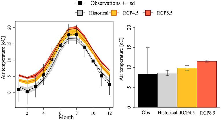
Figure 3. Ensemble mean, monthly air temperature in 2 m height (in °C) at Gotland Deep (BY15) calculated from four regional climate simulations: historical period (1976–2005) (solid black line) and future period (2069-2098) according to RCP 4.5 and RCP 8.5 scenarios (solid orange and red lines, respectively). The colored shaded areas denote the range between minus and plus one standard deviation among the ensemble members. In addition, observations and their standard deviations are shown (black squares and vertical thin bars).
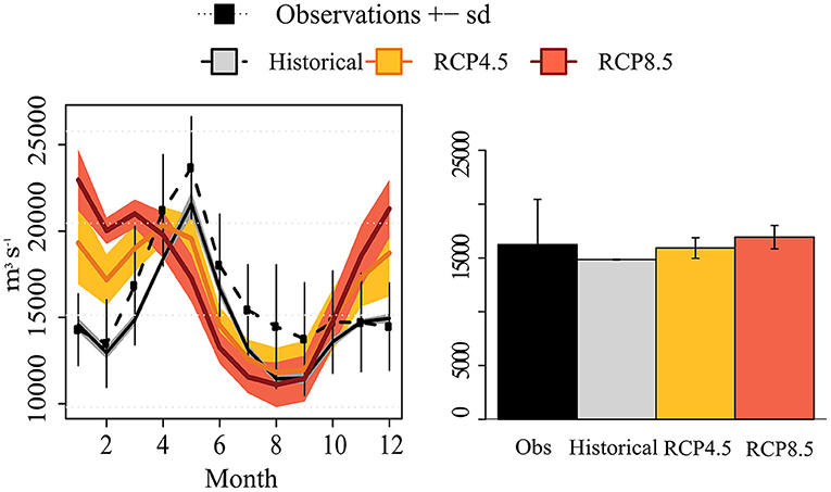
Figure 4. Ensemble mean, monthly (left), and annual (right) runoff (in m3 s−1) for the Baltic Sea calculated from four hydrological model simulations: historical period (1976–2005) (solid black line in the left panel and gray bar in the right panel) and future period (2069–2098) according to RCP 4.5 (orange) and RCP 8.5 (red) scenarios, respectively. The colored shaded areas in the left panel denote the range between minus and plus one standard deviation among the ensemble members. In addition, observations and their standard deviations are shown (dashed black line with squares and vertical thin bars in the left panel and black bar in the right panel).
Nutrient Load Scenarios
Climate projections for the Baltic Sea are carried out under the three nutrient load scenarios described below, spanning a range of plausible future socio-economic conditions from the most optimistic to the worst scenario. During the historical period (1976–2005), the observed nutrient loads from the Baltic Environmental Database (BED) are used (http://nest.su.se/bed/).
• Baltic Sea Action Plan (BSAP) scenario (HELCOM, 2013). In this scenario, nutrient loads from rivers and atmospheric deposition in the different sub-basins will linearly decrease after 2012 from the current values (average 2010–2012) as estimated by Svendsen et al. (2015) to the maximum allowable input defined by the BSAP until 2020. After 2020, nutrient loads will remain constant until 2098.
• Reference scenario. In this scenario, E-HYPE projections for future nutrient loads (2006–2098) under the two different greenhouse gas concentration scenarios (RCP 4.5 and RCP 8.5) are used, assuming no socio-economic changes compared to the historical period (1976–2005). Hence, e.g., land and fertilizer usage, soil properties and sewage water treatment in each sub-basin are assumed to be unchanged over time. Atmospheric deposition is also assumed to be constant in time. Only the impacts of the changing climate on air temperature and precipitation over the Baltic Sea catchment area are considered.
• Worst Case scenario. In this scenario, a socio-economic impact factor, corresponding to the worst case, is multiplied to the future nutrient loads calculated with E-HYPE under the RCP 4.5 and RCP 8.5 scenarios (2006–2098). The socio-economic impact factor summarizes the impact from Shared Socio-economic Pathways (SSPs) (O'Neill et al., 2014) on current nutrient loads and atmospheric deposition, based on the downscaling of the global trends of socio-economic drivers to the Baltic Sea region (Zandersen et al., in press). Following the assumptions of the global SSPs, changes in nitrogen and phosphorus loads were calculated from the regional assumptions, e.g., on population growth, changes in agricultural practices such as land and fertilizer use and expansion of sewage water treatment plants. To represent the worst conditions, the impact factor from the so-called SSP5 was selected, representing the changes caused by a “fossil-fuelled development” scenario.
In all three scenarios, nutrient loads into the Baltic Sea will decrease in the future following the historical efforts toward nutrient load reductions starting in the 1980s (Figure 5). However, in the Worst Case scenario the loads are close to the average observed loads during 1976–2005. Monthly and long-term changes in the Reference and Worst Case scenarios follow river runoff changes caused by changing climate. Only the BSAP scenario assumes that climate change does not counteract nutrient load abatement strategies. Hence, the latter is an optimistic scenario.
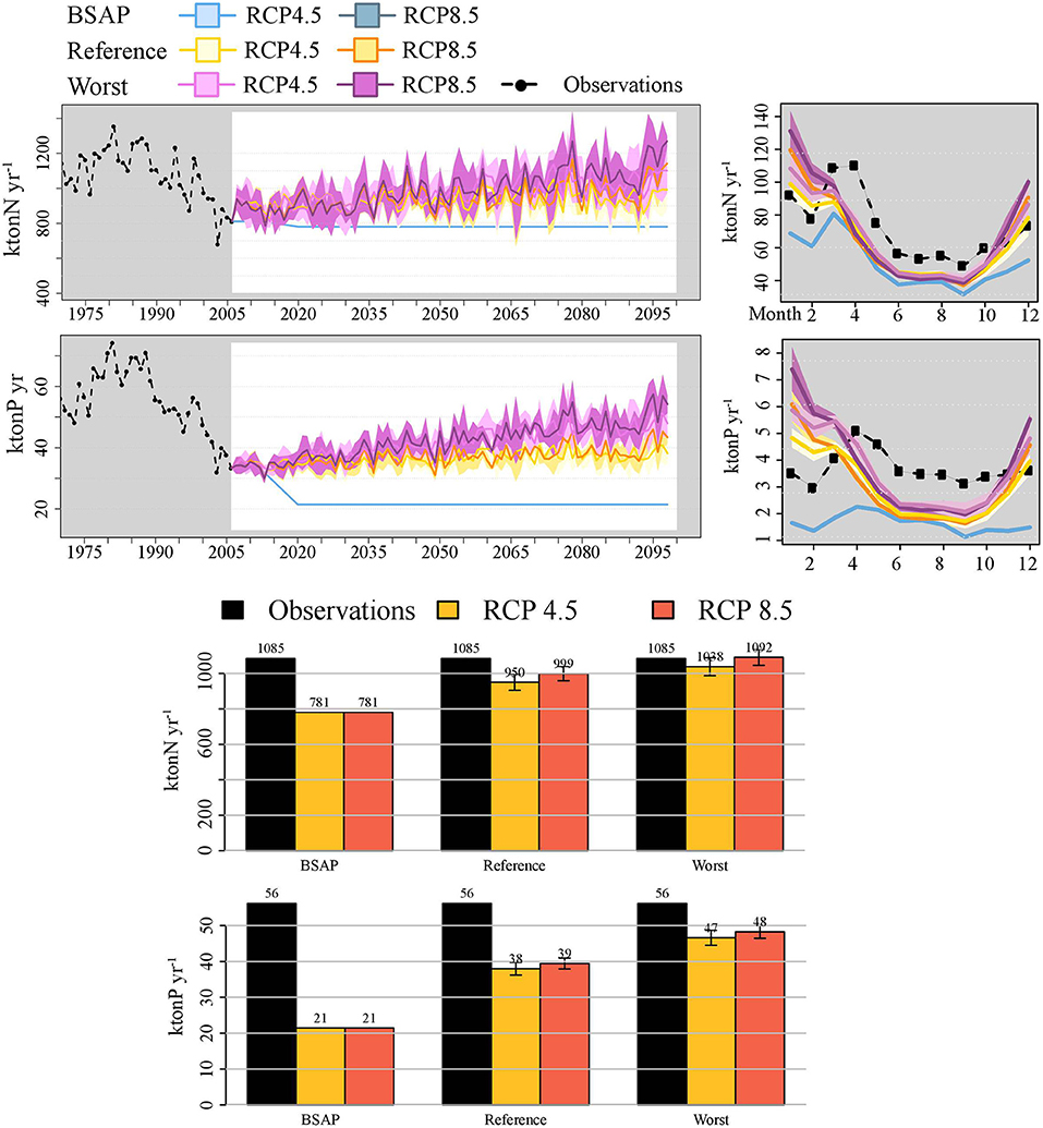
Figure 5. Observed and projected ensemble mean of the total bioavailable nutrient loads (nitrogen and phosphorus) to the Baltic Sea between 1970 and 2098 (upper, left panels), mean seasonal cycle (upper, right panels) and annual mean loads (lower). Shown is the sum of loads from rivers, point sources and atmosphere. Results were calculated from four hydrological model simulations during the historical (1976–2005) and future (2069–2098) periods according to the RCP 4.5 and RCP 8.5 scenarios combined with three nutrient loads scenarios (BSAP, Reference, and Worst Case). The colored shaded areas denote the standard deviations among the ensemble members. Observations are shown as black dashed lines with squares.
Experimental Setup
The combinations of future climate scenarios (RCP 4.5 and RCP 8.5; for Model C only RCP 4.5 is available) calculated with the four GCMs and three socio-economic scenarios (BSAP, Reference and Worst Case) result in an ensemble of 21 scenario simulations (Table 2). All simulations for the historical period 1975–2005 driven by the four GCMs start from the same initial conditions in March 1975, which were obtained from a long hindcast simulation starting in 1850. The latter simulation was driven by reconstructed atmospheric, hydrological, and nutrient loads estimated from available historical observations (Meier et al., 2012c, 2018).
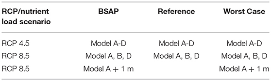
Table 2. List of experiments (for details see text).
In addition, two sensitivity experiments for Model A under RCP 8.5 (BSAP and Worst Case) with a 1 m higher sea level during 2006–2098 were performed. In these two experiments the thickness of the uppermost layer was increased by 1 m following Meier et al. (2017) (i.e., a 4 m surface layer instead of 3 m). Hence, during the start of the sensitivity experiment the difference between the depth of the pycnocline and the depth of the sills in the entrance area of the Baltic Sea (Figure 1) did not change compared to the scenario simulation with unchanged mean sea level.
The impacts of climate and nutrient load changes on the marine ecosystem were quantified by comparing various future scenarios (2069–2098) with the historical period of the GCM driven climate simulations (1976–2005). We focus our analysis on the changes and uncertainties of water temperature and salinity as well as on environmentally important indicators, such as nitrogen fixation, primary production and hypoxic areas. For more evaluation results of the model simulations during the historical period, the reader is referred to an accompanying paper (Saraiva et al., 2018a) and to the supplementary material (Figure S1).
To quantify the uncertainties (spread) in the projected changes we follow the approach by Ruosteenoja et al. (2016). For the evaluation of uncertainty in the 30 years mean changes between the future (2069–2098) and historical (1976–2005) climates, we calculate and compare the variances of changes caused by each of the different factors: GCMs (), RCPs (), nutrient loads (), and global mean sea level rise ().
and
etc.,
with the mean value for all four indices n, m, k and l
and
etc.. N = 4, m = 2, K = 3, and L = 2 are the total numbers of global models, greenhouse gas concentration scenarios, nutrient load scenarios and sea level rise sensitivity experiments (no change and + 1 m), respectively. Nm, k, l ≤ 4 is the number of global models for the greenhouse gas concentration scenario m, the nutrient load scenario k and the sea level rise experiment l, and so on. Global mean sea level sensitivity experiments exist only for Model A together with either BSAP or Worst Case. Further, for Model C the RCP 8.5 scenario is not available. Hence, the number of terms in the equations above are smaller than the product N x M x K x L. Mk, l, n is defined correspondingly. In case of , the variances caused by global models are summed for all combinations of RCPs, nutrient loads and sea level rise experiments. Finally, all variances of changes in primary production, nitrogen fixation and hypoxic area are normalized by the corresponding variance based upon the changes in all 23 simulations i.e., we calculated fractions of the total variances.
Results of Future Projections
Temperature and Salinity
According to our ensemble, water temperature will increase with time as a direct consequence of the increase in air temperature projected by the GCMs (Figure 6). The ensemble mean of the Baltic Sea volume averaged temperature change (and its standard deviation) between future (2069–2098) and historical (1976–2005) conditions amounts to 1.6 ± 0.5°C in RCP 4.5 and to 2.7 ± 0.4°C in RCP 8.5. The largest changes in SST follow the spatial pattern detected in previous projections (Meier et al., 2012a), with pronounced warming during the summers in the northern Baltic Sea (see Figure S3).
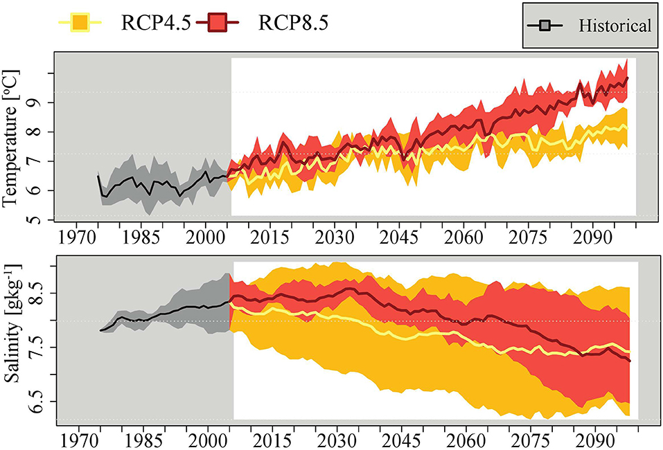
Figure 6. Ensemble mean volume averaged temperature (in °C) and salinity (in g kg−1) as a function of time for 1975–2098 in the two climate scenarios, RCP 4.5 (orange) and RCP 8.5 (red). The colored shaded areas denote the standard deviations among the ensemble members.
Due to the projected increased river runoff, the volume averaged salinity decreases in all scenario simulations at the end of the century (Figure 6). However, the differences between GCMs are substantial (Figure 10). The largest salinity decline of about −1.5 g kg−1 in future relative to the historical period is found in the regionalization of Model C (IPSL-CM5A-MR). In contrast, Model B (EC-EARTH) shows first a slight increase in salinity until approximately 2030. During the second half of the 21st century salinity decreases, and the differences between RCP 4.5 and RCP 8.5 are smaller than the results given by other models. Thus, the range of salinity changes is large and, consequently, uncertainties in salinity projections are substantial and greater than those in the temperature projections (see section on Impact of Global Mean Sea Level Rise below). For Model C, the greenhouse gas concentration scenario RCP 8.5 was not simulated because a river runoff projection from E-HYPE was not available. Hence, the two ensembles of salinity projections shown in Figure 6 should not be used to compare uncertainties in RCP 4.5 and RCP 8.5 projections.
Although the absolute values of the changes in temperature and salinity vary between the two greenhouse gas concentration scenarios, the shape of the average vertical profile does not change significantly (see Figure S2).
Biogeochemical Variables
Both changing nutrient loads and changing physical conditions have impacts on biogeochemical processes and nutrient cycling in the water column and sediments. In case of the Reference scenario, the model projects that the ensemble mean of the annual nutrient concentrations averaged for the entire Baltic Sea will change (between 1976–2005 and 2069–2098) under the RCP 4.5 scenario with about −62% for ammonium, +10% for nitrate and −24% for phosphate (Figure 7, middle panel). Decreased phosphate concentrations result in decreased primary production (−13%) and nitrogen fixation (−20%). As during the spring bloom nitrate is not completely consumed (due to lacking phosphate), nitrate concentration increases (+10%) relative to the average of the historical period. Average oxygen concentration is projected to slightly decrease by about −1%, probably because of the increasing water temperature. Following the decrease in phosphate and primary production, hypoxic area is 9% smaller than during the historical period.
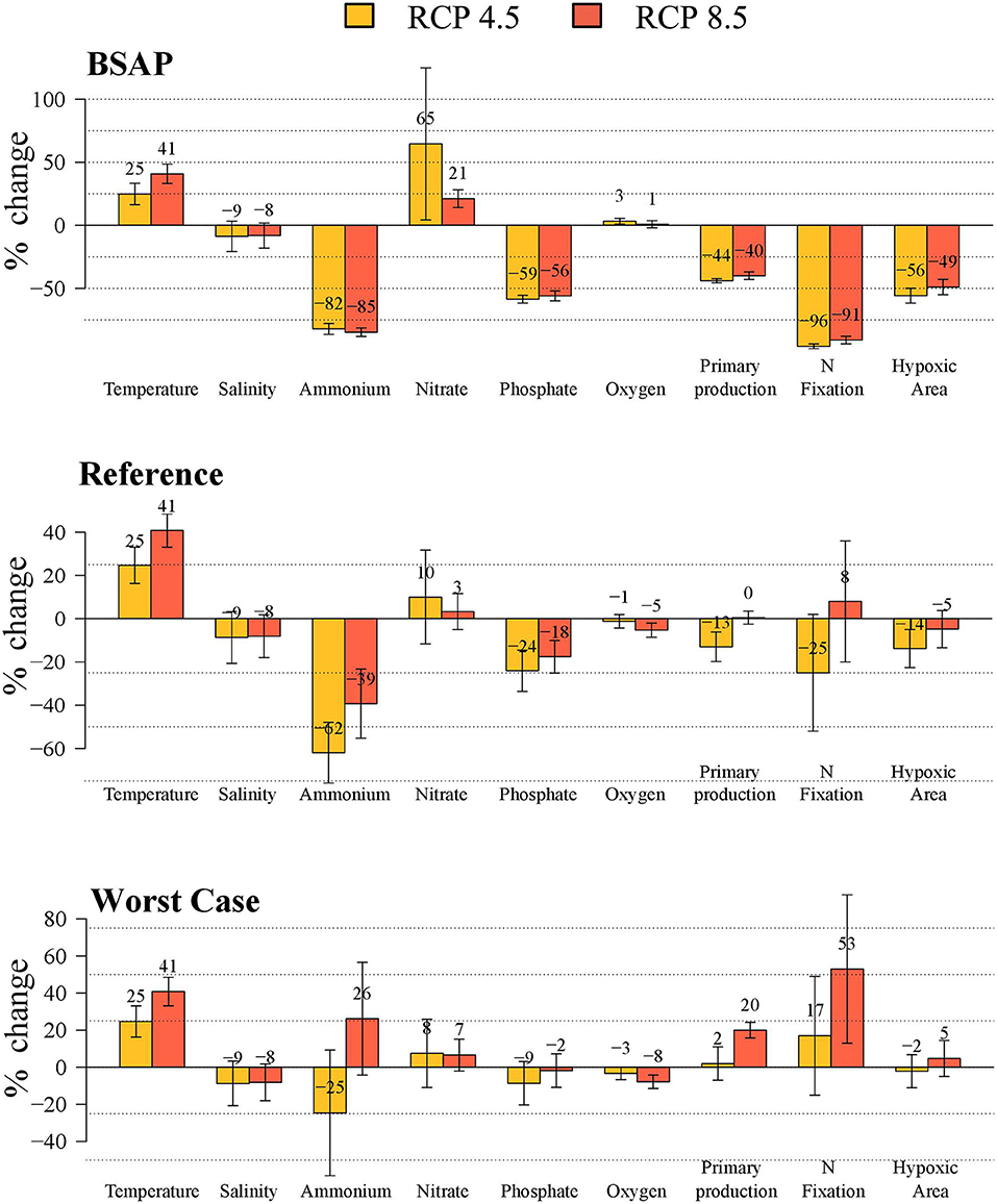
Figure 7. Relative ensemble mean volume averaged, 30 years mean changes between the future (2069–2098) and historical (1976–2005) periods in temperature, salinity, nutrient and oxygen concentrations, primary production, nitrogen fixation and hypoxic areas in the entire Baltic Sea under the different climate and nutrient load scenarios: BSAP (upper panel), Reference (middle panel) and Worst Case (bottom panel). The relative temperature changes are based on temperatures in °C. In addition, the standard deviations of changes among the ensemble members are shown.
In BSAP, the even larger reduction in nutrient loads results in a considerable reduction in primary production (−44%), nitrogen fixation (−96%), and hypoxic area (−32%) under the RCP 4.5 scenario (Figure 7, upper panel) whereas in the Worst Case primary production (+2%), nitrogen fixation (+22%) and hypoxic area (−3%) remain either unchanged or increase under the same greenhouse gas concentration scenario (Figure 7, lower panel). Hence, changes in nutrient supply, in particular phosphorus, control the long-term response of eutrophication, biogeochemical fluxes and oxygen conditions in the deep water.
Under the warmer RCP 8.5 scenario, the response of the biogeochemical cycles to changes in nutrient loads (BSAP, Reference, Worst Case) is similar compared to RCP 4.5 (Figure 7). The projected changes in temperature, salinity and other variables result in larger eutrophication, productivity and oxygen depletion. However, the impact of changing climate is more pronounced in case of high nutrient loads like the Worst Case scenario than in case of low nutrient loads like the BSAP scenario. This conclusion follows from the finding that under the BSAP the differences between the projections driven by RCP 4.5 and RCP 8.5 are smaller than for the corresponding differences under the Worst Case. Hence, the response of biogeochemical cycles to warming climate under various nutrient load scenarios is non-linear. This result found in our ensemble study becomes particularly noticeable by analyzing summer bottom oxygen and hydrogen sulfide concentrations (Figure 8). For BSAP, the differences in summer bottom oxygen concentrations at the end of the century between RCP 4.5 and RCP 8.5 scenarios are small. Hydrogen sulfide does not occur even in the deepest parts of the Baltic Sea. However, in the Worst Case scenario large areas suffer from hydrogen sulfide with considerably larger concentrations in RCP 8.5 compared to RCP 4.5.
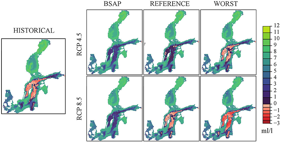
Figure 8. Historical (1976–2005) and projected future (2069–2098) ensemble mean summer bottom oxygen concentrations (in mL L−1) in three nutrient load (BSAP, Reference and Worst Case) and two greenhouse gas concentration scenarios (RCP 4.5 and 8.5). Hydrogen sulfide concentrations are represented by negative oxygen concentrations (1 mL H2S L−1 = −2 mL O2 L−1).
Under the BSAP, projected hypoxic area in the RCP 4.5 and RCP 8.5 scenario simulations is about −32 and −37% of present day, respectively (Figure 7). Hypoxic area is successively larger with increasing nutrient loads and increasing warming. In the combination of the Worst Case and RCP 8.5 scenarios, about 80% of the Baltic proper will have, on average, anoxic bottom conditions during summer. However, even in the latter scenario simulation, hypoxic area is still slightly smaller or about the same as under present conditions (Figures 7, 9).
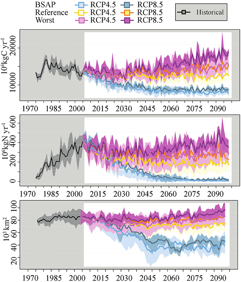
Figure 9. Temporal evolution of ensemble mean volume averaged primary production (in 106 kg C year−1, upper panel) and nitrogen fixation (in 106 kg N year−1, middle panel), and hypoxic area (in 103 km2, lower panel) in the entire Baltic Sea during 1975–2098 and their standard deviations (ensemble spread) among ensemble members. For all combinations of the two greenhouse gas concentration scenarios (RCP 4.5 and 8.5) and the three nutrient load scenarios (BSAP, Reference and Worst Case) the ensemble mean and spread were calculated from four regionalized global climate simulations.
Independent of the climate scenario, RCP 4.5 or RCP 8.5, primary production and nitrogen fixation increase in future climate under the Worst Case scenario and decrease under the BSAP (Figure 7). Again, whether the response of the biogeochemical fluxes will be affected by changing climate depends on the nutrient loads. For instance, under the Worst Case scenario nitrogen fixation will increase by 22 and 56% in RCP 4.5 and RCP 8.5, respectively, whereas under the BSAP nitrogen fixation will approximately vanish in both cases.
In Figure 9, the temporal evolutions of primary production, nitrogen fixation and hypoxic area are shown. The standard deviation among the four ensemble members is large. However, at the end of the century the results for the Worst Case (or even for the Reference scenario) and the BSAP are clearly distinguishable.
Impact of Global Mean Sea Level Rise
In this section, we compare the results of the scenario simulations with those of the two sensitivity experiments with a 1 m higher mean sea level (Model A under the RCP 8.5 and BSAP or Worst Case scenarios plus 1 m). At the end of the century, the volume averaged salinity in the experiment with 1 m higher mean sea level (Model A under the RCP 8.5 scenario plus 1 m) is approximately 1.5 g kg−1 higher than in the corresponding scenario simulation without changing the mean sea level (Model A under the RCP 8.5) (Figure 10). The higher mean sea level causes increases in both frequency and magnitude of saltwater inflows due to the greater water depth in the Danish straits causing an increase in the salt flux between Kattegat and Arkona Basin (cf. Meier et al., 2017). Hence, at the end of the simulation period salinity in the Baltic Sea is higher and the vertical stratification is larger compared to the corresponding scenario simulation without mean sea level rise. For comparison, in our ensemble the ranges of projected salinities at the end of the century under both RCP 4.5 and RCP 8.5 scenarios amount to approximately 2 g kg−1 (Figure 6). As wind fields do not change significantly (not shown), these ranges are mainly explained by differences in the projected river runoff.
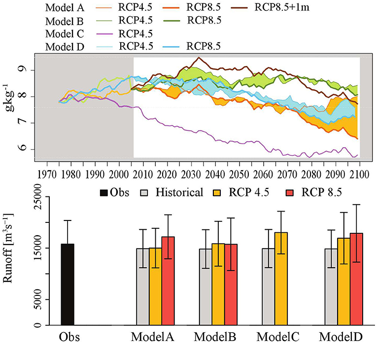
Figure 10. Upper panel: Temporal evolution of volume averaged salinity (in g kg−1) in the entire Baltic Sea during 1975–2098 in various climate scenarios (RCP 4.5 and 8.5) using four global climate models: MPI-ESM-LR (Model A); EC-EARTH (Model B); IPSL-CM5A-MR (Model C); HadGEM2-ES (Model D). Note, a scenario simulation driven by Model C and RCP 8.5 does not exist. A sensitivity experiment forced by Model A under the RCP 8.5 scenario assuming a 1 m higher mean sea level is also shown. Lower panel: Annual mean river runoff (in m3 s−1) in the scenario simulations and observations (1976–2005).
As a consequence of a higher mean sea level, oxygen concentrations of salt water inflows are higher causing an improved ventilation of the deep water. However, since stratification is getting stronger, the vertical flux of oxygen from the surface to the bottom is reduced in bottom areas along the slopes of the deeper sub-basins, that are not directly affected by salt water inflows and that drop below the rising halocline. The latter process causes larger areas of hypoxia. The differences in the projected hypoxic areas at the end of the century between simulations with 1 m higher mean sea level and without changing mean sea level are less than 10% indicating a modest sensitivity to mean sea level change (Figure 11). Hence, the results suggest that the differing future nutrient loads will dominate the uncertainties in the hypoxic area projections if the range of nutrient loads is defined by the Worst Case and BSAP scenarios (cf. Figure 7). In addition, the uncertainty caused by the global models is considerable and significantly larger than the uncertainty due to greenhouse gas concentration scenarios (either RCP 4.5 or RCP 8.5).
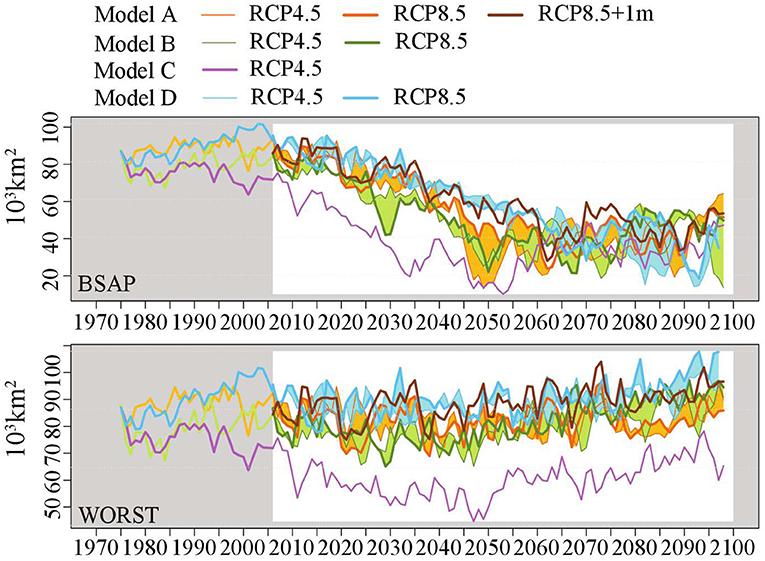
Figure 11. As the upper panel in Figure 10 but for hypoxic area under the BSAP and Worst Case scenarios.
Discussion
In this study, an ensemble of 21 scenario simulations driven by four different GCMs and two sensitivity experiments on sea level rise was performed, by combining different future climate scenarios and nutrient load projections for the 21st century.
Compared to earlier Baltic Sea studies, the new features of this study are:
• simulations for the period 1850–2098 including a spin-up with reconstructed forcing for 1850–1975;
• consistent simulations without bias correction except for the wind speed and mean runoff;
• dynamical downscaling of four GCMs with the aim of estimating the impact of climate model uncertainties on the Baltic Sea properties;
• revised, more plausible nutrient load scenarios taking the latest observations into account;
• two greenhouse gas concentration scenarios corresponding to RCP 4.5 and RCP 8.5;
• improved version of the coupled physical-biogeochemical model of the Baltic Sea (Eilola et al., 2009); and
• improved versions of the global models from the Coupled Model Intercomparison Project 5 (CMIP5) of the IPCC (Stocker et al., 2013).
The sensitivity experiments are not scenario simulations following Stocker et al. (2013) because the 1 m higher mean sea level was applied as being constant in time during 2006–2098. The reason for this experimental setup is that the Baltic Sea model RCO has a linearized free sea surface following Killworth et al. (1991) that does not permit long-term changes in the mean sea surface height (Meier et al., 1999). Hence, our experiments overestimate the effect of the increasing global mean sea level and, thus, overestimate the increasing salinity in the Baltic Sea (Figures 10, 11). In our sensitivity experiments, a 1 m higher mean sea level was chosen because this value is close to the high-end scenario simulation results at the end of the 21st century (Stocker et al., 2013). As projections of global mean sea level rise are rather uncertain (Stocker et al., 2013), the aim of our sensitivity experiments is only to illustrate a possible maximum effect of increasing global mean sea level that has been neglected in all previous scenario simulations of the Baltic Sea (Meier et al., 2017).
The projected ensemble mean change in salinity under the RCP 4.5 scenario amounts to −0.7 g kg−1 compared with that of the historical period, with a considerable ensemble spread among the different GCMs. Under the RCP 8.5 scenario, the ensemble mean change of the three GCMs amounts to −0.6 g kg−1. However, since the ensemble excludes the model that shows the greatest projected salinity change under the RCP 4.5 scenario (Model C), we assume that under RCP 8.5 the change of the ensemble mean will also be greater if Model C is included (Figure 10). Hence, our ensemble is too small and the uncertainties, inter alia, in the salinity projections might be underestimated.
Substantial uncertainties in future projections for the Baltic Sea are caused by the driving climate models, e.g., those for salinity due to uncertainties in projected river runoff and global mean sea level rise (Figure 10), cf. Meier et al. (2017). In RCP 4.5 and RCP 8.5, the projected river runoff varies between 1 and 21% and between 6 and 20%, respectively, explaining the considerable uncertainties in the projected salinity (Meier and Kauker, 2003b; their Figure 7), which are much greater than the natural variability (Meier and Kauker, 2003a). Uncertainties in salinity and stratification affect biogeochemical fluxes and hypoxic areas (Eilola et al., 2011). For instance, the vertical flux of oxygen between the well-oxygenated surface layer and the deep water is controlled by vertical stratification (Väli et al., 2013). Hence, deficiencies in climate models have considerable impacts on the water balance of the Baltic Sea that cannot be neglected in regional projections (Meier et al., 2011a). However, in our multi-model ensemble study the resulting uncertainties in biogeochemical fluxes, such as primary production and nitrogen fixation, and hypoxic areas are still significantly smaller than the differences caused by the different nutrient load scenarios, i.e., Worst Case and BSAP (Table 3). In addition, the uncertainties caused by unknown greenhouse gas concentration (RCP 4.5 and RCP 8.5) and global mean sea level rise scenarios are also smaller than the differences between nutrient load scenarios. Thus, we found an overwhelming impact of the various nutrient load scenarios on the changing biogeochemical cycles in the Baltic Sea. For (1) primary production and (2) nitrogen fixation and hypoxic area, the second largest uncertainties are based on the choice of the greenhouse gas concentration scenario (RCP 4.5 or RCP 8.5) and climate model uncertainties (calculated from four GCMs), respectively (Table 3). As one of the main uncertainties in the salinity projections is caused by the differing river runoff projections between the driving GCMs (Table 3, Figure 10), we conclude that projections of nitrogen fixation and hypoxic area suffer from shortcomings in the simulated water cycles. For changes in primary production, the magnitude of the temperature increase also plays an important role. In addition, our sensitivity experiment indicates that the uncertainty in salinity changes due to global mean sea level rise has an important impact on nitrogen fixation and hypoxic area as well. The latter result is in agreement with Meier et al. (2017).
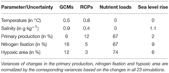
Table 3. Uncertainties expressed as standard deviations in temperature and salinity and variances of 30 years mean changes between the future (2069–2098) and historical (1976–2005) climates in primary production, nitrogen fixation and hypoxic area caused by GCMs, RCPs, nutrient loads, and global mean sea level rise (only model A, BSAP, and Worst Case, see Table 2).
In this study, only results from greenhouse gas concentration scenarios RCP 4.5 and RCP 8.5 were analyzed. RCP 2.6, at the lower end of the IPCC greenhouse gas concentration scenarios, corresponding to the goal of a global temperature rise limited to < 2°C, was not studied. Hence, in our ensemble the range of warming in the Baltic Sea region is smaller than that of the full range of global scenario simulations.
Further, we have not investigated the uncertainties caused by the shortcomings in the RCMs of the Baltic Sea. Eilola et al. (2011) compared three different coupled physical-biogeochemical models for the Baltic Sea under the present climate conditions. They concluded that the models reproduce much of the biogeochemical cycling in the Baltic proper in hindcast simulations during 1970–2005. However, uncertainties caused by the assumptions about the bioavailable fractions of nutrient loads from land and parameterizations of the key biogeochemical processes were considerable. The same models were also used in an ensemble of scenario simulations for 1961–2099 (Meier et al., 2011a, 2012b,c; Neumann et al., 2012). Within the latter studies, substantially differing nutrient load scenarios and driving GCMs were applied, making a direct comparison with our results impossible. As only two driving GCMs were used and as the impact of global mean sea level rise was neglected, the previously published ensemble spread in salinity was smaller than that found in our study. Uncertainties in the projections of the hypoxic area were about as large as those presented in the ensemble of scenario simulations of this study. Hence, future projections of the Baltic Sea ecosystem require multi-model ensembles of regional and global climate models to allow a suitable estimate of uncertainties.
The assumption that the ensemble spread due to natural variability at the end of the 21st century is small compared to the other uncertainties might be wrong on the regional scale. In a forthcoming study, the sources of uncertainty will be studied in more detail.
Conclusions
From the model results of this study, we draw the following conclusions:
(1) Implementation of the BSAP will lead to a significantly improved ecosystem state of the Baltic Sea irrespective of the driving GCM because changing climate will not counteract nutrient load reductions.
(2) The main driver of eutrophication is external nutrient loads. Climate change (mainly warming and global mean sea level rise) may amplify eutrophication. The response of biogeochemical fluxes, such as primary production and nitrogen fixation, and deep water oxygen conditions to changing climate depend on the nutrient load scenario. In the case of high (low) nutrient loads, the impact of the changing climate would be considerable (negligible). However, the impacts of the changing climate within the range of the considered greenhouse gas concentration scenarios (RCP 4.5 and RCP 8.5) on biogeochemical cycles will be smaller than the impacts of the considered nutrient load changes (BSAP, Reference, Worst Case).
(3) Substantial uncertainties of future projections for the Baltic Sea are caused by the driving GCMs. For instance, salinity projections differ considerably due to the uncertainties in the projected river runoff and global mean sea level rise. Hence, for future projections an ensemble of various driving GCMs is necessary. This study also shows that dynamical downscaling is a useful tool because local drivers of marine biogeochemical cycling, such as nutrient load changes, are still more important than the estimated uncertainties caused by deficiencies of the climate models. Despite the large uncertainties caused by climate models, we were able to draw a conclusion concerning the impact of the BSAP in future climates (see Conclusion no. 1).
Data Availability Statement
Observations from the Baltic Environmental Database (BED) are publicly available from http://nest.su.se/bed. Model codes and data used for the analysis of this study are available from the authors upon request.
Author Contributions
For the BalticAPP proposal, concept and design of the study was developed by HM. SS performed the scenario simulations with the help of HM, AH, CD, MG, RH, HA, and KE. SS visualized and analyzed the model results. HM and SS wrote the text of the manuscript. All co-authors helped with comments, contributed to the manuscript revision, read and approved the submitted version.
Funding
The research presented in this study is part of the Baltic Earth program (Earth System Science for the Baltic Sea region, see http://www.baltic.earth) and was funded by the BONUS BalticAPP (Well-being from the Baltic Sea—applications combining natural science and economics) project which has received funding from BONUS, the joint Baltic Sea research and development programme (Art 185), funded jointly from the European Union's Seventh Programme for research, technological development and demonstration and from the Swedish Research Council for Environment, Agricultural Sciences and Spatial Planning (FORMAS, grant no. 942-2015-23). Support by FORMAS within the project Cyanobacteria life cycles and nitrogen fixation in historical reconstructions and future climate scenarios (1850-2100) of the Baltic Sea (grant no. 214-2013-1449) and by the CERES project, which has received funding from the European Union's Horizon 2020 research and innovation programme under grant agreement no. 678193, is acknowledged. In addition, SS would like to acknowledge the support by Fundação para a Ciência e a Tecnologia, Portugal (SFRH/BPD/120279/2016) in the later phase of this project.
Conflict of Interest Statement
The authors declare that the research was conducted in the absence of any commercial or financial relationships that could be construed as a potential conflict of interest.
Acknowledgments
The observational data used for the weighting, analysis of nutrient content and lateral boundary conditions are open access and were extracted from the Baltic Environmental Database (BED, http://nest.su.se/bed) at Stockholm University and all data providing institutes (listed at http://nest.su.se/bed/ACKNOWLE.shtml) are kindly acknowledged. BED contains observations, inter alia, from the national, long-term environmental monitoring programs such as the Swedish Ocean Archive (SHARK, http://sharkweb.smhi.se) operated by the Swedish Meteorological and Hydrological Institute (SMHI) or the German Baltic Sea monitoring data archive (http://iowmeta.io-warnemuende.de) operated by the Leibniz Institute for Baltic Sea Research Warnemünde (IOW). The paper is based upon an earlier manuscript by Saraiva et al. (2018b).
Supplementary Material
The Supplementary Material for this article can be found online at: https://www.frontiersin.org/articles/10.3389/feart.2018.00244/full#supplementary-material
References
Ahtiainen, H., and Öhman, H. C. (2014). Ecosystem Services in the Baltic Sea: Valuation of Marine and Coastal Ecosystem Services in the Baltic Sea, vol. 563 of Report TemaNord. Copenhagen: Nordic Council of Ministers.
Almroth-Rosell, E., Eilola, K., Hordoir, R., Meier, H. E. M., and Hall, P. O. J. (2011). Transport of fresh and resuspended particulate organic material in the Baltic Sea – a model study. J. Mar. Syst. 87, 1–12. doi: 10.1016/j.jmarsys.2011.02.005
BACC II Author Team (2015). Second Assessment of Climate Change for the Baltic Sea Basin. Cham: Regional Climate Studies, Springer. doi: 10.1007/978-3-319-16006-1
Belkin, I. M. (2009). Rapid warming of large marine ecosystems. Prog. Oceanogr. 81, 207–213. doi: 10.1016/j.pocean.2009.04.011
Block, K., and Mauritsen, T. (2013). Forcing and feedback in the MPI-ESM-LR coupled model under abruptly quadrupled CO2. J. Adv. Model. Earth Syst. 5, 676–691. doi: 10.1002/jame.20041
Carstensen, J., Andersen, J. H., Gustafsson, B. G., and Conley, D. J. (2014). Deoxygenation of the Baltic Sea during the last century. Proc. Natl. Acad. Sci. U. S. A. 111, 5628–5633. doi: 10.1073/pnas.1323156111
Christensen, J. H., Kjellström, E., Giorgi, F., Lenderink, G., and Rummukainen, M. (2010). Weight assignment in regional climate models. Clim. Res. 44, 179–194. doi: 10.3354/cr00916
Conley, D. J., Björck, S., Bonsdorff, E., Carstensen, J., Destouni, G., Gustafsson, B. G., et al. (2009). Hypoxia-related processes in the Baltic Sea. Environ. Sci. Technol. 43, 3412–3420. doi: 10.1021/es802762a
Dahlgren, P., Landelius, T., Kallberg, P., and Gollvik, S. (2016). A high-resolution regional reanalysis for Europe. Part 1: three- dimensional reanalysis with the regional HIgh-Resolution Limited-Area Model (HIRLAM). Quart. J. R. Meteorol. Soc. 142, 698(A), 2119–2131. doi: 10.1002/qj.2807
Déqué, M., Somot, S., Sanchez-Gomez, E., Goodess, C., Jacob, D., Lenderink, G., et al. (2012). The spread amongst ENSEMBLES regional scenarios: regional climate models, driving general circulation models and interannual variability. Clim. Dyn. 38, 951–964. doi: 10.1007/s00382-011-1053-x
Dieterich, C., Schimanke, S., Wang, S., Väli, G., Liu, Y., Hordoir, R., et al. (2013). Evaluation of the SMHI Coupled Atmosphere-Ice-Ocean Model RCA4-NEMO. vol. 47 of Report Oceanography, SMHI, Norrköping, Sweden
Donnelly, C., Arheimer, B., Capell, R., Dahné, J., and Strömqvist, J. (2013). “Regional overview of nutrient load in Europe – challenges when using a large-scale model approach, E-HYPE,”in Proceedings of H04, IAHS-IAPSO-IASPEI Assembly. Gothenburg, Sweden, IHS Publ. 361, 49–58.
Donnelly, C., Greuell, W., Andersson, J., Gerten, D., Pisacane, G., Roudier, P., et al. (2017). Impacts of climate change on European hydrology at 1.5, 2 and 3 degrees mean global warming above preindustrial level. Climatic Change 143, 13–26. doi: 10.1007/s10584-017-1971-7.
Döscher, R., and Meier, H. E. M. (2004). Simulated sea surface temperature and heat fluxes in different climates of the Baltic Sea. Ambio 33, 242–248. doi: 10.1579/0044-7447-33.4.242
Eilola, K., Almroth-Rosell, E., Dieterich, C., Fransner, F., Höglund, A., and Meier, H. E. M. (2012). Modeling nutrient transports and exchanges of nutrients between shallow regions and the open Baltic Sea in present and future climate. Ambio 41, 586–599. doi: 10.1007/s13280-012-0317-y
Eilola, K., Gustafsson, B. G., Kuznetsov, I., Meier, H. E. M., Neumann, T., and Savchuk, O. P. (2011). Evaluation of biogeochemical cycles in an ensemble of three state-of-the-art numerical models of the Baltic Sea. J. Mar. Syst. 88, 267–284. doi: 10.1016/j.jmarsys.2011.05.004
Eilola, K., Mårtensson, S., and Meier, H. E. M. (2013). Modeling the impact of reduced sea ice cover in future climate on the Baltic Sea biogeochemistry. Geophys. Res. Lett. 40, 149–154. doi: 10.1029/2012GL054375
Eilola, K., Meier, H. E. M., and Almroth, E. (2009). On the dynamics of oxygen, phosphorus and cyanobacteria in the Baltic Sea; A model study. J. Mar. Syst. 75, 163–184. doi: 10.1016/j.jmarsys.2008.08.009.
Friedland, R., Neumann, T., and Schernewski, G. (2012). Climate change and the Baltic Sea action plan: model simulations on the future of the western Baltic Sea. J. Mar. Syst. 105, 175–186. doi: 10.1016/j.jmarsys.2012.08.002
Giorgi, F., and Mearns, L. O. (1991). Approaches to the simulation of regional climate change: a review. Rev. Geophys. 29, 191–216.
Gröger, M., Dieterich, C., Meier, H. E. M., and Schimanke, S. (2015). Thermal air–sea coupling in hindcast simulations for the North Sea and Baltic Sea on the NW European shelf. Tellus A Dyn. Meteorol. Oceanogr. 67:26911. doi: 10.3402/tellusa.v67.26911
Gustafsson, B. G., Schenk, F., Blenckner, T., Eilola, K., Meier, H. E. M., Müller-Karulis, B., et al. (2012). Reconstructing the development of Baltic Sea eutrophication 1850–2006. Ambio 41, 534–548. doi: 10.1007/s13280-012-0318-x
Hawkins, E., and Sutton, R. (2009). The potential to narrow uncertainty in regional climate predictions. Bull. Am. Meteorol. Soc. 90, 1095–1108. doi: 10.1175/2009BAMS2607.1
Hazeleger, W., Wang, X., Severijns, C., Stefănescu, S., Bintanja, R., Sterl, A., et al. (2012). EC-Earth V2. 2: description and validation of a new seamless earth system prediction model. Clim. Dyn. 39, 2611–2629. doi: 10.1007/s00382-011-1228-5
Heavens, N. G., Ward, D. S., and Natalie, M. M. (2013). Studying and projecting climate change with earth system models. Nat. Educ. Know. 4:4
HELCOM (2013). “Copenhagen ministerial declaration,” in HELCOMMinisterial Meeting, Copenhagen, Denmark.
Hieronymus, J., Eilola, K., Hieronymus, M., Meier, H. E. M., Saraiva, S., and Karlson, B. (2018). Causes of simulated long-term changes in phytoplankton biomass in the Baltic proper: a wavelet analysis. Biogeosciences 15, 5113–5129. doi: 10.5194/bg-15-5113-2018
Hourdin, F., Foujols, M.-A., Codron, F., Guemas, V., Dufresne, J.-L., Bony, S., et al. (2013). Impact of the LMDZ atmospheric grid configuration on the climate and sensitivity of the IPSL-CM5A coupled model. Clim. Dyn. 40, 2167–2192. doi: 10.1007/s00382-012-1411-3
Hundecha, Y., Arheimer, B., Donnelly, C., and Pechlivanidis, I. (2016). A regional parameter estimation scheme for a pan-European multi-basin model. J. Hydrol. Region. Stud. 6, 90–111. doi: 10.1016/j.ejrh.2016.04.002.
Jacob, D., Petersen, J., Eggert, B., Alias, A., Christensen, O. B., Bouwer, L. M., et al. (2014). EURO-CORDEX: new high-resolution climate change projections for European impact research. Reg. Environ. Change 14, 563–578. doi: 10.1007/s10113-013-0499-2.
Jones, C. D., Hughes, J. K., Bellouin, N., Hardiman, S. C., Jones, G. S., Knight, J., et al. (2011). The HadGEM2-ES implementation of CMIP5 centennial simulations. Geosci. Model Dev. 4, 543–570. doi: 10.5194/gmd-4-543-2011
Killworth, P. D., Webb, D. J., Stainforth, D., and Paterson, S. M. (1991). The development of a free-surface Bryan–Cox–Semtner ocean model. J. Phys. Oceanogr. 21, 1333–1348.
Kjellström, E., Nikulin, G., Hansson, U. L. F., Strandberg, G., and Ullerstig, A. (2011). 21st century changes in the European climate: uncertainties derived from an ensemble of regional climate model simulations. Tellus A Dyn. Meteorol. Oceanog. 63, 24–40. doi: 10.1111/j.1600-0870.2010.00475.x
Kupiainen, M., Jansson, C., Samuelsson, P., Jones, C., Willén, U., Wang, S., et al. (2014). Rossby Centre Regional Atmospheric Model, RCA4, Rossby Center News Letter. SMHI, Norrköping, Sweden. Available online at : http://www.smhi.se/en/Research/Research-departments/climate-research-rossby-centre2-552/1.16562 (Accessed August 14, 2018)
Madec, G. (2016). NEMO ocean engine. version 3.6 stable. Note du Pôle de modélisation. Institut Pierre-Simon Laplace (IPSL)-LOCEAN. Paris: The NEMO team. Available online at : https://www.nemo-ocean.eu/wp-content/uploads/NEMO_book.pdf (Accessed August 17, 2018)
Marti, O., Braconnot, P., Dufresne, J.-L., Bellier, J., Benshila, R., Bony, S., et al. (2010). Key features of the IPSL ocean atmosphere model and its sensitivity to atmospheric resolution. Clim. Dyn. 34, 1–26. doi: 10.1007/s00382-009-0640-6
Mathis, M., Elizalde, A., and Mikolajewicz, U. (2018). Which complexity of regional climate system models is essential for downscaling anthropogenic climate change in the Northwest European Shelf? Clim. Dyn. 50, 2637–2659. doi: 10.1007/s00382-017-3761-3
Meehl, G. A., Washington, W. M., Ammann, C. M., Arblaster, J. M., Wigley, T. M. L., and Tebaldi, C. (2004). Combinations of natural and anthropogenic forcings in twentieth-century climate. J. Clim. 17, 3721–3727. doi: 10.1175/1520-0442
Meier, H. E., Kjellström, E., and Graham, L. P. (2006). Estimating uncertainties of projected Baltic Sea salinity in the late 21st century. Geophys. Res. Lett. 33:488. doi: 10.1029/2006GL026488
Meier, H. E. M. (2002a). Regional ocean climate simulations with a 3D ice-ocean model for the Baltic Sea. Part 1: model experiments and results for temperature and salinity. Clim. Dyn. 19, 237–253. doi: 10.1007/s00382-001-0224-6
Meier, H. E. M. (2002b). Regional ocean climate simulations with a 3D ice-ocean model for the Baltic Sea. Part 2: Results for sea ice. Clim. Dyn. 19, 255–266. doi: 10.1007/s00382-001-0225-5
Meier, H. E. M. (2006). Baltic Sea climate in the late twenty-first century: a dynamical downscaling approach using two global models and two emission scenarios. Clim. Dyn. 27, 39–68. doi: 10.1007/s00382-006-0124-x.
Meier, H. E. M. (2007). Modeling the pathways and ages of inflowing salt-and freshwater in the Baltic Sea. Estuar. Coast. Shelf Sci. 74, 610–627. doi: 10.1016/j.ecss.2007.05.019
Meier, H. E. M., Andersson, H. C., Arheimer, B., Blenckner, T., Chubarenko, B., Donnelly, C., et al. (2012c). Comparing reconstructed past variations and future projections of the Baltic Sea ecosystem – first results from multi-model ensemble simulations. Environ. Res. Lett. 7:034005. doi: 10.1088/1748-9326/7/3/034005
Meier, H. E. M., Andersson, H. C., Eilola, K., Gustafsson, B. G., Kuznetsov, I., Müller-Karulis, B., et al. (2011a). Hypoxia in future climates: a model ensemble study for the Baltic Sea. Geophys. Res. Lett. 38:L24608. doi: 10.1029/2011GL049929
Meier, H. E. M., Döscher, R., Coward, A. C., Nycander, J., and Döös, K. (1999). RCO - Rossby Centre Regional Ocean Climate Model: Model Description (version 1.0) and First Results From the Hindcast Period 1992/93. Reports Oceanography No.26, SMHI, Norrköping.
Meier, H. E. M., Döscher, R., and Faxén, T. (2003). A multiprocessor coupled ice-ocean model for the Baltic Sea: application to salt inflow. J. Geophys. Res. Oceans 108:3273. doi: 10.1029/2000JC000521
Meier, H. E. M., Döscher, R., and Halkka, A. (2004). Simulated distributions of Baltic Sea-ice in warming climate and consequences for the winter habitat of the Baltic ringed seal. Ambio 33, 249–256. doi: 10.1579/0044-7447-33.4.249
Meier, H. E. M., Eilola, K., and Almroth, E. (2011c). Climate-related changes in marine ecosystems simulated with a three-dimensional coupled biogeochemical-physical model of the Baltic Sea. Clim. Res. 48, 31–55. doi: 10.3354/cr00968
Meier, H. E. M., Eilola, K., Almroth-Rosell, E., Schimanke, S., Kniebusch, M., Höglund, A., et al. (2018). Disentangling the impact of nutrient load and climate changes on Baltic Sea hypoxia and eutrophication since 1850. Clim. Dyn. 1–22. doi: 10.1007/s00382-018-4296-y
Meier, H. E. M., Höglund, A., Döscher, R., Andersson, H., Löptien, U., and Kjellström, E. (2011b). Quality assessment of atmospheric surface fields over the Baltic Sea of an ensemble of regional climate model simulations with respect to ocean dynamics. Oceanologia 53, 193–227. doi: 10.5697/oc.53-1-TI.193
Meier, H. E. M., Höglund, A., Eilola, K., and Almroth-Rosell, E. (2017). Impact of accelerated future GMSL rise on hypoxia in the Baltic Sea. Clim. Dyn. 49:163–172. doi: 10.1007/s00382-016-3333-y
Meier, H. E. M., Hordoir, R., Andersson, H., Dieterich, C., Eilola, K., Gustafsson, B. G., et al. (2012a). Modeling the combined impact of changing climate and changing nutrient loads on the Baltic Sea environment in an ensemble of transient simulations for 1961-2099. Clim. Dyn. 39, 2421–2441. doi: 10.1007/s00382-012-1339-7
Meier, H. E. M., and Kauker, F. (2003a). Modeling decadal variability of the Baltic Sea: 2. Role of freshwater inflow and large-scale atmospheric circulation for salinity. J. Geophys. Res. Oceans 108. doi: 10.1029/2003JC001799
Meier, H. E. M., and Kauker, F. (2003b). Sensitivity of the Baltic Sea salinity to the freshwater supply. Clim. Res. 24, 231–242. doi: 10.3354/cr024231.
Meier, H. E. M., Müller-Karulis, B., Andersson, H. C., Dieterich, C., Eilola, K., Gustafsson, B. G., et al. (2012b). Impact of climate change on ecological quality indicators and biogeochemical fluxes in the Baltic Sea: a multi-model ensemble study. Ambio 41, 558–573. doi: 10.1007/s13280-012-0320-3
Moss, R. H., Edmonds, J. A., Hibbard, K. A., Manning, M. R., Rose, S. K., Van Vuuren, D. P., et al. (2010). The next generation of scenarios for climate change research and assessment. Nature 463, 747–756. doi: 10.1038/nature08823
Neumann, T. (2010). Climate-change effects on the Baltic Sea ecosystem: a model study. J. Mar. Syst. 81, 213–224. doi: 10.1016/j.jmarsys.2009.12.001
Neumann, T., Eilola, K., Gustafsson, B., Müller-Karulis, B., Kuznetsov, I., Meier, H. E. M., et al. (2012). Extremes of temperature, oxygen and blooms in the Baltic Sea in a changing climate. Ambio 41, 574–585. doi: 10.1007/s13280-012-0321-2.
Omstedt, A., Edman, M., Claremar, B., Frodin, P., Gustafsson, E., Humborg, C., et al. (2012). Future changes in the Baltic Sea acid–base (pH) and oxygen balances. Tellus B Chem. Phys. Meteorol. 64:19586. doi: 10.3402/tellusb.v64i0.19586
Omstedt, A., Gustafsson, B., Rodhe, J., and Walin, G. (2000). Use of Baltic Sea modelling to investigate the water cycle and the heat balance in GCM and regional climate models. Clim. Res. 15, 95–108. doi: 10.3354/cr015095
O'Neill, B. C., Kriegler, E., Riahi, K., Ebi, K. L., Hallegatte, S., Carter, T. R., et al. (2014). A new scenario framework for climate change research: the concept of shared socioeconomic pathways. Climatic Change 122, 387–400. doi: 10.1007/s10584-013-0905-2
Räisänen, J., Hansson, U., Ullerstig, A., Döscher, R., Graham, L. P., Jones, C., et al. (2004). European climate in the late twenty-first century: regional simulations with two driving global models and two forcing scenarios. Clim. Dyn. 22, 13–31. doi: 10.1007/s00382-003-0365-x
Ruosteenoja, K., Jylhä, K., and Kämäräinen, M. (2016). Climate projections for Finland under the RCP forcing scenarios. Geophysica 51, 17–50.
Ryabchenko, V., Karlin, L., Isaev, A., Vankevich, R., Eremina, T., Molchanov, M., et al. (2016). Model estimates of the eutrophication of the Baltic Sea in the contemporary and future climate. Oceanology 56, 36–45. doi: 10.1134/S0001437016010161
Saraiva, S., Meier, H. E. M., Andersson, H., Höglund, A., Dieterich, C., Hordoir, R., et al. (2018a). Baltic Sea ecosystem response to various nutrient load scenarios in present and future climates. Clim. Dyn. 1–19. doi: 10.1007/s00382-018-4330-0
Saraiva, S., Meier, H. E. M., Andersson, H., Höglund, A., Dieterich, C., Hordoir, R., et al. (2018b). Uncertainties in projections of the Baltic Sea ecosystem driven by an ensemble of global climate models. Earth Syst. Dynam. Discuss. 1–30. doi: 10.5194/esd-2018-16
Savchuk, O. P. (2002). Nutrient biogeochemical cycles in the Gulf of Riga: scaling up field studies with a mathematical model. J. Mar. Syst. 32, 253–280. doi: 10.1016/S0924-7963(02)00039-8
Schimanke, S., Dieterich, C., and Meier, H. E. M. (2014). An algorithm based on sea-level pressure fluctuations to identify major Baltic inflow events. Tellus A Dyn. Meteorol. Oceanograp. 66:23452. doi: 10.3402/tellusa.v66.23452
Schimanke, S., and Meier, H. E. M. (2016). Decadal-to-centennial variability of salinity in the Baltic Sea. J. Climate 29, 7173–7188. doi: 10.1175/JCLI-D-15-0443.1
Sjöberg, B. (1992). Sea and Coast – National Atlas of Sweden, SMHI. Stockholm: Swedish Meteorological and Hydrological Institute (SMHI).
Stålnacke, P., Grimvall, A., Sundblad, K., and Tonderski, A. (1999). Estimation of riverine loads of nitrogen and phosphorus to the Baltic Sea, 1970–1993. Environ. Monitor. Assess. 58, 173–200. doi: 10.1023/A:1006073015871
Stevens, B., Giorgetta, M., Esch, M., Mauritsen, T., Crueger, T., Rast, S., et al. (2013). Atmospheric component of the MPI-M Earth System Model: ECHAM6. J. Adv. Model. Earth Syst. 5, 146–172. doi: 10.1002/jame.20015
Stocker, T., Qin, D., Plattner, G.-K., Alexander, L., Allen, S., Bindoff, N., et al. (2013). “Technical summary”, in Climate Change 2013: the Physical Science Basis. Contribution of Working Group I to the Fifth Assessment Report of the Intergovernmental Panel on Climate Change, eds. T. Stocker, G. K. Qin, M. Plattner, S.K. Tignor, J. Allen, A. Boschung, et al. (Cambridge: Cambridge University Press)
Svendsen, L. M., Pyhälä, M., Gustafsson, B., Sonesten, L., and Knuuttila, S. (2015). Inputs of Nitrogen and Phosphorus to the Baltic Sea. HELCOM Core Indicator Report. Helsinki Commission, Helsinki, Finland.
Uppala, S. M., Kållberg, P. W., Simmons, A. J., Andrae, U., Bechtold, V. D. C., Fiorino, M., et al. (2005). The ERA40 reanalysis. Q. J. R. Meteorol. Soc. 131, 2961–3012. doi: 10.1256/qj.04.176
Väli, G., Meier, H. E. M., and Elken, J. (2013). Simulated halocline variability in the Baltic Sea and its impact on hypoxia during 1961-2007. J. Geophys. Res. 118, 6982–7000. doi: 10.1002/2013JC009192
Wang, S., Dieterich, C., Döscher, R., Höglund, A., Hordoir, R., Meier, H. E. M., et al. (2015). Development and evaluation of a new regional coupled atmosphere–ocean model in the North Sea and Baltic Sea. Tellus A Dyn. Meteorol. Oceanograp. 67:24284. doi: 10.3402/tellusa.v67.24284
Wilcke, R. A. I., and Bärring, L. (2016). Selecting regional climate scenarios for impact modelling studies. Environ. Modell. Software 78, 191–201. doi: 10.1016/j.envsoft.2016.01.002
Keywords: Baltic Sea, nutrients, eutrophication, climate change, future projections, uncertainties, ensemble simulations
Citation: Saraiva S, Meier HEM, Andersson H, Höglund A, Dieterich C, Gröger M, Hordoir R and Eilola K (2019) Uncertainties in Projections of the Baltic Sea Ecosystem Driven by an Ensemble of Global Climate Models. Front. Earth Sci. 6:244. doi: 10.3389/feart.2018.00244
Received: 11 October 2018; Accepted: 17 December 2018;
Published: 09 January 2019.
Edited by:
Tomas Halenka, Charles University, CzechiaReviewed by:
Matthias Prange, University of Bremen, GermanyJofre Carnicer, University of Barcelona, Spain
Copyright © 2019 Saraiva, Meier, Andersson, Höglund, Dieterich, Gröger, Hordoir and Eilola. This is an open-access article distributed under the terms of the Creative Commons Attribution License (CC BY). The use, distribution or reproduction in other forums is permitted, provided the original author(s) and the copyright owner(s) are credited and that the original publication in this journal is cited, in accordance with accepted academic practice. No use, distribution or reproduction is permitted which does not comply with these terms.
*Correspondence: H. E. Markus Meier, markus.meier@io-warnemuende.de