Unraveling the Physics of the Yellowstone Magmatic System Using Geodynamic Simulations

Reuber, Georg S.; Kaus, Boris J. P.; Popov, Anton A.; Baumann, Tobias S.

doi:10.3389/feart.2018.00117

ORIGINAL RESEARCH article

Front. Earth Sci., 20 August 2018
Sec. Volcanology
Volume 6 - 2018 | https://doi.org/10.3389/feart.2018.00117

Unraveling the Physics of the Yellowstone Magmatic System Using Geodynamic Simulations

Georg S. Reuber¹^*

Boris J. P. Kaus^1,2,3

Anton A. Popov¹

Tobias S. Baumann¹

¹Institute of Geosciences, Johannes Gutenberg University, Mainz, Germany
²Center for Computational Sciences Mainz, Johannes Gutenberg University, Mainz, Germany
³Volcanoes, Atmospheres and Magmatic Open Systems Research Center, Johannes Gutenberg University, Mainz, Germany

The Yellowstone magmatic system is one of the largest magmatic systems on Earth, and thus an ideal location to study magmatic processes. Whereas previous seismic tomography results could only image a shallow magma reservoir, a recent study using more seismometers showed that a second and massive partially molten mush reservoir exists above the Moho (Huang et al., 2015). To understand the measurable surface response of this system to visco-elasto-plastic deformation, it is thus important to take the whole system from the mantle plume up to the shallow magma reservoirs into account. Here, we employ lithospheric-scale 3D visco-elasto-plastic geodynamic models to test the influence of parameters such as the connectivity of the reservoirs and rheology of the lithosphere on the dynamics of the system. A gravity inversion is used to constrain the effective density of the magma reservoirs, and an adjoint modeling approach reveals the key model parameters affecting the surface velocity. Model results show that a combination of connected reservoirs with plastic rheology can explain the recorded slow vertical surface uplift rates of around 1.2 cm/year, as representing a long term background signal. A geodynamic inversion to fit the model to observed GPS surface velocities reveals that the magnitude of surface uplift varies strongly with the viscosity difference between the reservoirs and the crust. Even though stress directions have not been used as inversion parameters, modeled stress orientations are consistent with observations. However, phases of larger uplift velocities can also result from magma reservoir inflation which is a short term effect. We consider two approaches: (1) overpressure in the magma reservoir in the asthenosphere and (2) inflation of the uppermost reservoir prescribed by an internal kinematic boundary condition. We demonstrate that the asthenosphere inflation has a smaller effect on the surface velocities in comparison with the uppermost reservoir inflation. We show that the pure buoyant uplift of magma bodies in combination with magma reservoir inflation can explain (varying) observed uplift rates at the example of the Yellowstone volcanic system.

1. Introduction

Understanding magmatic systems has been a long-standing research topic within the solid-Earth geosciences. To understand the underlying processes better, several volcanic areas on the Earth have been geophysically monitored, geologically mapped and interpreted. At the same time numerical or analog models have been developed to unravel the mechanical driving forces. As a result, a paradigm shift has happened over the last decade, and we now know that magmatic systems are lithospheric-scale systems composed by many smaller pulses of melt (Cashman et al., 2017). Yet, our understanding of the physics of such systems remains somewhat limited.

Classically, models have been used to link surface deformation data to the depth, size and overpressure of a magma reservoir. If the rocks are elastic and the magma reservoir is spherical and embedded in an infinite halfspace, an analytical solution exists (Mogi, 1958). This approach has been widely applied, for example, to show that surface uplift above the Hekla volcano (Iceland) is consistent with a reservoir at 8 km depth (Lanari et al., 1998), to constrain the depth of the magma source beneath Etna (Kjartansson and Gronvold, 1983), or to reproduce cyclicity in ground deformation at Montserrat as a result of pressurization of a dike-conduit system (Hautmann et al., 2009). The Mogi approach has been extended to account for topographic effects and crustal heterogeneities in both 2D (e.g., Trasatti et al., 2003) and 3D (e.g., Manconi et al., 2010). Furthermore, the analytical solution has been extended to include viscous effects, for example by Del Negro et al. (2009), who compare the temperature-dependent visco-elastic to the elastic solution and show that the required overpressures to fit observed uplift at Etna is about a third lower in the visco-elastic case, which is more consistent with the lithospheric stress state. Such overpressures may nevertheless exceed the yield strength of crustal host rocks, in which case the material deforms plastically rather than (visco-)elastic. An evaluation of such elasto-plastic effects shows that these produce higher uplift rates for the same overpressure (Currenti et al., 2010; Gerbault et al., 2012). Davis et al. (1974) argue that at Hawaii this will likely result in fracturing of the host rock around the magma reservoir and result in a net of pathways, which is inconsistent with spherical source of overpressure. Battaglia and Segall (2004) also point out the limitations of the assumption that magmatic bodies are spherical, and show that whereas uplift rates can often be reproduced with a spherical models, the resulting depth of the source is incorrect.

Many of these previous studies focus on upper-crustal magma reservoirs and consider a single pulse of magma. Yet, as magmatic systems are likely formed by many pulses, it is important to take those into account, as done by Degruyter and Huber (2014) who investigated the effect of pulses on the style and frequency of eruptions and provide scaling laws for mechanical locking of the magma reservoir due to thermal cooling. The work by Annen (2011) and Annen and Sparks (2002) demonstrates that subsequent magmatic pulses help keep the system hot and partially molten, which may significantly change the mechanics of magma transport once a critical amount of heating has occurred (Karlstrom et al., 2017).

Seismic tomography studies of magmatic systems give important insights into the 3D structure at depth. Yet, interpreting these results in terms of melt content with depth is not straightforward as the seismic wavelengths themselves are several kilometers in size and the distribution of seismometers is often sub-optimal. Some attempts have been made to perform a joint inversion in which thermal models and melting parameterizations are combined with tomographic inversions. Results for Montserrat show that melt fractions obtained in this manner are substantially larger than those directly inferred from interpreting seismic data (Paulatto et al., 2012). Yet, whereas this gives important new insights in the geometry of the system, it does not tell much about the physics of magmatic systems, which is the focus of our work.

We use the Yellowstone magmatic system (Wyoming, US) as a case study, as it is one of the best studied volcanic systems on Earth that has a significant hazard potential having ejected around 1000 km³ during the last eruption (~640 ka). A comprehensive summary on the evolution and petrology of the Yellowstone magmatic system is given by Christiansen (2001). Geophysically, Yellowstone is a well-studied area. Figure 1 summarizes the available observational data constraints that include gravity anomaly, GPS uplift velocities for a period of high activity from 2003 to 2008 (Vasco et al., 2007), and the orientation of the minimum principal stress (Waite and Smith, 2004). Furthermore, Smith and Braile (1994) and Smith et al. (2009) give an overview over the seismic tomography, earthquakes, surface uplift and stress orientations within and at the system. Even though the exact geometry of the Yellowstone magmatic system remains under discussion, recent publications, (e.g., Huang et al., 2015 based on seismic tomography), suggest that the system extends over lithospheric scales ranging from a deep mantle plume over a magma reservoir within the lower crust at a depth of 40 km (~46,000 km³) to a shallow magma reservoir (~10,000 km³) in the upper crust at a depth of 15 km. A 2D numerical study of the Yellowstone magmatic system has been published very recently (Colón et al., 2018). They investigated the effect of rheological changes in the magma reservoir during the emplacement of the magma bodies. A thermal mantle plume emplaced in the asthenosphere results after several Ma in strong magmatic reworking of the crust. Due to rheological contrasts at the crust-mantle (Moho) transition and the lower-upper crustal (Conrad) transition, magmas may stall at such locations and experience chemical differentiation (e.g., fractional differentiation from basalt to rhyolite). As a conclusion the authors highlight the importance of taking the large scale dynamics (lithosphere scale) and complex rheologies of crust and mantle into account while studying magmatic systems. However, with the current computing capacity it is unfeasible to systematically study the full evolution of such systems in 3D. Our aims are to fit the present day geophysical observations by instantaneous numerical models and to understand the processes that influence these observables. In particular we want to investigate the effect of a visco-elasto-plastic rheology on the surface observables in combination with the effect of inflation of the magmatic chambers. We retrieve the present day geometry by interpreting the tomographic results and converting the velocity anomalies into a 3D geometry of the magma reservoirs. We then perform instantaneous 3D mechanical models of the system, taking the visco-elasto-plastic rheology of rocks into account and compare model predictions with present day data. An instantaneous numerical model is usually described as the solution of the numerical model after one time step, as such the model is essentially not time dependent. Since we include elasticity in the models we refer to the term instantaneous as the solution of the numerical model after reaching elastic relaxation (see Supplementary Material in Appendix 2).

FIGURE 1

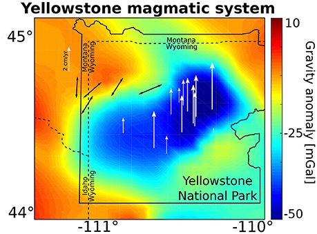
Figure 1. Overview of some geophysical data for Yellowstone used in this work. The area corresponds to the computational domain presented in this work. Colors indicate the bouguer gravity anomaly in the area referenced to the anomaly close to the boundary of the area. Data is taken from the online archive of the Pan American Center for Earth and Environmental Sciences (PACES) and DeNosaquo et al. (2009). White vertical arrows indicate the GPS velocities during a period of high activity from 2003 to 2008 (Vasco et al., 2007). Black arrows represent the orientation of the minimum principal stress (σ₃) (taken from Waite and Smith (2004) and references therein).

Recently, it was shown that geodynamic inversion frameworks can serve as a powerful tool to link geophysical observations with thermo-mechanically consistent deformation models to infer rheological properties of the crust and lithosphere (Baumann et al., 2014; Baumann and Kaus, 2015). Here, we apply a gradient-based adjoint inversion technique combined with data assimilation (Ratnaswamy et al., 2015) to constrain the dynamics of the Yellowstone magmatic system, and discuss whether full 3D models are required for such systems, or 2D models are sufficient. In the following sections we describe the underlying numerical method (Kaus et al., 2016), the adjoint inversion framework, and provide some background on the thermodynamical modeling that is incorporated in this study. We present two different approaches to simulate the effect of inflation of a crustal magma reservoir, while simultaneously taking the buoyancy effect of the lithospheric-scale magmatic system into account. We systematically test the effect of rheological complexities on surface uplift and incorporate the most successful of these models in an inversion approach to constrain the material parameters from data.

2. Methods

2.1. Physics and Numerics

In this work we solve for the conservation of momentum and mass in a compressible formulation. For a domain Ω with a boundary ∂Ω the underlying coupled equation system is given by:

\begin{array}{l} \frac{\partial τ_{i j}}{\partial x_{j}} - \frac{\partial P}{\partial x_{i}} + ρ g_{i} & = 0, & (1) \end{array}

\begin{array}{l} \frac{1}{K} \frac{D P}{D t} + \frac{\partial v_{i}}{\partial x_{i}} & = 0 . & (2) \end{array}

Here x_i(i = 1, 2, 3) denotes Cartesian coordinates, v_i is the velocity vector, P is the pressure, τ_ij is the Cauchy deviator stress tensor, ρ is the density, g_i is the gravity acceleration vector, K is the elastic bulk modulus, and D/Dt stands for the material time derivative. Here and below we imply the Einstein summation convention. Due to a moderate time span of the models considered in this work (~10⁴ years), we ignore the effect of temperature advection and diffusion, and therefore omit the solution of the energy balance equation. On a free-slip boundary with a normal vector pointing in i-th direction we enforce the following condition:

\begin{array}{l} v_{i} = \bar{v}, \frac{\partial v_{j}}{\partial x_{i}} = 0, j \neq i, & (3) \end{array}

where $\bar{v}$ is the normal velocity component. On a no-slip boundary we apply v_i = 0.

The deviatoric stress tensor is defined by a set of visco-elasto-plastic constitutive equations of the form:

\begin{array}{l} {\dot{ε}}_{i j} = {\dot{ε}}_{i j}^{e l} + {\dot{ε}}_{i j}^{v s} + {\dot{ε}}_{i j}^{p l} = \frac{{\overset{◇}{τ}}_{i j}}{2 G} + \frac{τ_{i j}}{2 η} + \dot{γ} \frac{\partial Q}{\partial τ_{i j}}, & (4) \end{array}

\begin{array}{l} {\dot{ε}}_{i j} = \frac{1}{2} (\frac{\partial v_{i}}{\partial x_{j}} + \frac{\partial v_{j}}{\partial x_{i}}) - \frac{1}{3} \frac{\partial v_{k}}{\partial x_{k}} δ_{i j}, & (5) \end{array}

\begin{array}{l} {\overset{◇}{τ}}_{i j} & = \frac{\partial τ_{i j}}{\partial t} + τ_{i k} ω_{k j} - ω_{i k} τ_{k j}, & (6) \end{array}

\begin{array}{l} ω_{i j} & = \frac{1}{2} (\frac{\partial v_{i}}{\partial x_{j}} - \frac{\partial v_{j}}{\partial x_{i}}), & (7) \end{array}

where ${\overset{°}{ε}}_{i j}$ is the total deviatoric strain rate tensor, δ_ij is the Kronecker delta, the superscripts el, vs, and pl correspond to elastic, viscous, and plastic strain rate components, respectively, G is the elastic shear modulus, ${\overset{◇}{τ}}_{i j}$ is the Jaumann objective stress rate, ω_ij is the spin tensor, η is the creep viscosity, $\overset{°}{γ}$ is the magnitude of plastic strain rate (plastic multiplier), and Q is the plastic potential function. The effective viscosity is defined as a function of temperature, and strain-rate according to the dislocation creep mechanism (e.g., Kameyama et al., 1999):

\begin{array}{l} η = \frac{1}{2} {(B_{n})}^{- \frac{1}{n}} {({\dot{ε}}_{I I})}^{\frac{1}{n} - 1} \exp (\frac{E_{n}}{n R T}) . & (8) \end{array}

In the above expression, ${\dot{ε}}_{I I} = {(\frac{1}{2} {\dot{ε}}_{i j} {\dot{ε}}_{i j})}^{1 / 2}$ denotes the effective strain rate measure (square root of the second invariant), n is the stress exponent of the dislocation creep, and B_n, E_n, are the creep constant, and activation energy, respectively, R is the gas constant and T is temperature.

The magnitude of plastic multiplier is determined by enforcing the Drucker-Prager failure criterion (Drucker and Prager, 1952), given by:

\begin{array}{l} F = τ_{I I} - \sin (ϕ) P - \cos (ϕ) C \leq 0, & (9) \end{array}

where $τ_{I I} = {(\frac{1}{2} τ_{i j} τ_{i j})}^{1 / 2}$ is the effective deviatoric stress, ϕ is the friction angle, and C is the cohesion. To prevent the non-symmetry in the Jacobian matrix required by the adjoint method (see section 2.2) we use the lithostatic, instead of the fully dynamic pressure in the equation (9) in the simulations presented here. In this work we do not consider the effect of strain softening on the friction and cohesion parameters, since we solve instantaneous models. Softening would require time integration of the plastic strain. We adopt the dilatation-free non-associative Prandtl-Reuss flow rule, defined by the following plastic potential function:

\begin{array}{l} Q = τ_{I I} & (10) \end{array}

The dependence of the density field on the pressure and temperature is assumed to be given by a phase diagram (see section 2.3). The computation is performed externally using the consistent thermodynamic modeling with Perple_X. The feedback between density and influencing parameters is updated every nonlinear iteration.

We discretize and solve a coupled set of conservation and constitutive equations using 3D thermo-mechanical code LaMEM (Kaus et al., 2016), which is based on a staggered finite differences approximation (e.g., Harlow and Welsh, 1965; Gerya and Yuen, 2007; Tackley, 2008). The material properties are advected using a marker-and-cell method (Harlow and Welsh, 1965). To guarantee the computational stability for a large time step we employ a stabilized free surface boundary condition using the sticky-air approach (Kaus et al., 2010; Duretz et al., 2011). Nonlinearities are handled by a preconditioned Jacobian-Free Newton-Krylov (JFNK) method with line-search as implemented in the PETSc SNES nonlinear solver framework (Balay et al., 2016). The gravity anomaly computation adopted in LaMEM is based on a rectangular prism approximation (e.g., Plouff, 1976; Turcotte and Schubert, 2014). Further information regarding the computational efficiency of LaMEM, and the computational infrastructure used to compute the models is given in Supplementary Material in Appendix 1.

2.2. Adjoint Equations

The adjoint method for solving inverse problems is a powerful tool (e.g., Ismail-Zadeh et al., 2003). It is essentially based on a gradient-based inversion approach such as BFGS (Broyden-Fletcher-Goldfarb-Shanno) Quasi-Newton method (e.g., Ratnaswamy et al. (2015)). The gradients of the cost function with respect to model parameters are computed using an efficient (adjoint) procedure. The adjoint operator allows for the computation of all material gradients at once with the cost of only one linear solve. The adjoint gradients computation can be summarized as follows:

\begin{array}{l} ψ = {(J^{T})}^{- 1} {(\frac{\partial F}{\partial x})}^{T}, & (11) \end{array}

\begin{array}{l} \frac{d F}{d p} = - ψ^{T} \frac{\partial r}{\partial p}, & (12) \end{array}

where p is the model parameter vector, e.g., densities, viscosities, etc., J = ∂r/∂x is the Jacobian matrix of the forward problem, namely the derivative of the residual (r) with respect the solution vector (x), F is the objective (cost) function, quantifying the misfit between the observations and simulation results. The partial derivatives ∂r/∂p might be difficult to compute analytically. In these cases they can be approximated by finite differences. Numerical codes that solve the nonlinear equations by a Newton-Raphson method usually have the Jacobian matrix readily available. The adjoint gradient computation procedure can be rendered efficient since it only involves a single linear solve irrespective of the number of gradients.

The adjoint gradients can be used not only to solve the inverse problem but also to quantify the influence of model parameters on the model solution, i.e., to construct a scaling law (Reuber et al., in press). The essence of the adjoint scaling law can be briefly summarized as follows. We start with redefining the cost function (F) to be an arbitrary solution parameter of the forward model, e.g., (non-dimensional) velocity, instead of the misfit between the model and observation. Next, we assume that the actual scaling law for the solution parameter (F) can be approximated by the following multiplicative from:

\begin{array}{l} F \approx A_{F} p_{1}^{b_{1}} p_{2}^{b_{2}} \dots p_{n}^{b_{n}}, & (13) \end{array}

where A_F is the dimensionally-consistent prefactor. We can now conveniently compute the scaling exponents (b_i) of the approximate scaling law using the following expressions:

\begin{array}{l} b_{i} = \frac{d F}{d p_{i}} \frac{p_{i}}{F} . & (14) \end{array}

Here we use adjoint gradient procedure (Equations 11, 12) to estimate the derivatives of the solution parameter (F) with respect to models parameters (p).

2.3. Thermodynamic Modeling

To create a thermodynamically consistent model of the Yellowstone magmatic system, we use the thermodynamic modeling tool Perple_X (Connolly, 2009), version 6.7.4. Perple_X is freely available software which ensures the reproducibility of the results shown in this work. Furthermore, Perple_X has already proven its applicability to the field of thermomechanical modeling in multiple publications (e.g., Baumann et al., 2010; Angiboust et al., 2012; Koptev et al., 2016, in press). By Gibbs free energy minimization Perple_X computes material properties including phase changes. Here, we use it to compute rock densities as functions of pressure and temperature. The calculations were performed using the database of Holland and Powell (1998). As an approximation for the crust surrounding the Yellowstone magmatic reservoirs we take the average crust compositions from Rudnick and Gao (2003), described in Table 1.

TABLE 1

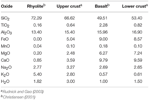
Table 1. Major element composition (in weight percent oxide) for all rock types used in this work.

To generate an initial guess for the effective densities of the magma reservoirs we used the method described in Bottinga and Weill (1970) for the whole rock data analysis described by Christiansen (2001). The used rock composition is shown in Table 1. In the gravity inversion, we vary the density between the completely molten and solid end-members to find a fit to the gravity signal.

3. Model Setup and Data Integration

The seismic study of Huang et al. (2015) represents the most recent seismic tomography model of the Yellowstone magmatic system, including a mantle plume and two distinct magma reservoirs in the lower and upper crust, respectively. We make use of their interpretation of the velocity anomalies and construct a 3D geometry of the magma reservoirs by digitizing the horizontal and vertical cross sections from Huang et al. (2015). The geometry on the horizontal and vertical sections was subsequently turned into a 3D model using the freely available software package geomIO (Baumann and Bauville, 2016). The computational domain includes the entire Yellowstone National Park and the eastern part of Idaho, which is roughly 110 km in East-West and 120 km in North-South direction, respectively (see Figure 2). The depth of the domain is restricted to 90 km, combined with an internal free surface at 0 km, overlain by a 10 km thick free-air layer (Crameri et al., 2012). The numerical resolution is 128 × 128 × 256 nodes in x, y and z direction. All boundaries are treated as free slip. The first two kilometers of the domain consist of a sediment layer. This layer represents a weak (potentially fractured due to hydrothermal activity, e.g., Morgan, 2007) cap. It is followed by 12 km of upper crust including the shallow magma reservoir. The lower crust includes the lower magma reservoir and extends 36 km in the vertical direction. The bottom of the domain is defined by the mantle lithosphere until a depth of 70 km and followed by asthenosphere. A connection of the mantle plume to the lower boundary simulates the connection to the deeper mantle. Additionally, connection channels are added to the model setup between the plume and the reservoirs, which can be activated to simulate weak connective areas, comparable to diking areas. Inflation of the magma reservoirs from the deeper mantle can be simulated by applying an overpressure at the lower bottom in the region of this connection. Alternatively, simultaneous deflation and inflation of the reservoirs in the lower and upper crust, respectively, can be simulated by activating a kinematic internal boundary condition inside the connection between the reservoirs.

FIGURE 2

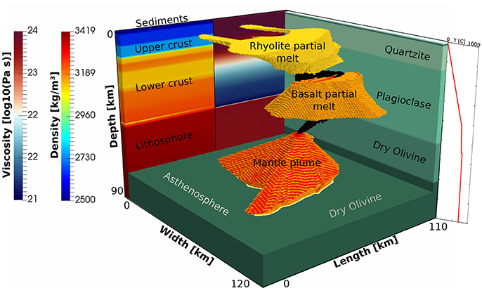
Figure 2. Model setup of the computational domain representing the lithospheric scale Yellowstone magmatic system. The positions and shapes of the phases are inspired by the seismic tomography data shown in Huang et al. (2015). Chambers and mantle plume are connected, while these connections can be active or made inactive (by giving it the same material properties as the host rock). Colors at the back of the domain show the density (left side) and viscosities (right side) at this location, while temperature along a 1D profile through the middle of the domain is shown at the right.

The temperature structure consists of three linear geotherms. In the sediment and the upper crust the geotherm is 15 K/km, followed by 3 K/km in the lower crust and lithosphere and 0.5 K/km for the rest of the domain. The surface temperature is assumed to be 0°C. We make the assumption that the surrounding material behaves like an “average” crust. As such the geotherm represents more the crust far away from the Yellowstone system. With this assumption the effect of the temperature in our models is of second order importance compared to the input of the thermodynamic model and the effective (constant) viscosity of the magma reservoirs, that already represents a composite hotter zone of partially molten rock. The effect of the temperature on the reservoirs is simulated by increasing the composite viscosity of the partially molten zones, representing a lower melt fraction. Our aim is to study the direct effect of the density and the viscosity on the dynamics of the system. One could in a future study of course directly invert for a temperature structure that would (nonlinear) influence the density, viscosity and even the size of the magma reservoir to fit the geophysical data. However, it is not straightforward to couple these parameters in a consistent way.

The initial setup is shown in Figure 2, while the employed material properties of all phases/rocktypes are summarized in Table 2.

TABLE 2

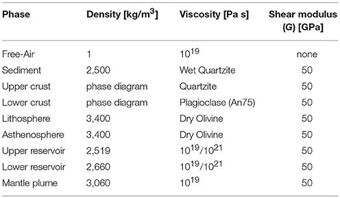
Table 2. Material properties used in this work.

4. Inverse Modeling Approach

For the inversions, we assume that the overall large-scale geometry of the Yellowstone magmatic system does not change, particularly with respect to the shape of the reservoirs and the structure of the layers. Since the buoyancy force is a major driving force controlling surface uplift, we will first constrain the density structure of the model by fitting the gravity anomaly (Figure 1). We change the effective densities of the two reservoirs, while keeping the densities of the surrounding crusts fixed (and computed from phase diagrams). The melt content of the mush reservoirs influences the effective density of the reservoirs. In this work we will not investigate the exact amount of melt in the magma reservoirs but rather invert directly for the effective density difference between the reservoir and surrounding rocks, as this is the key parameter that controls gravity anomalies. If the density difference between the crystal-free magma (i.e., melt phase) and the solid rock end-member is known, we can retrieve melt content from it (e.g., Bottinga and Weill, 1970). In doing this, we make the implicit assumption that the melt content within each of the reservoirs in our model setup is constant in space and time. In nature, it is quite possible that the melt content within the reservoirs varies as well, and our approach should thus be considered to only catch the first order effects on both the gravity field and the dynamics of the system. Gravity anomalies are well-known to be non-unique with respect to the relative density and geometry of the anomaly. Baumann et al. (2014) showed that using a joint geodynamic inversion of surface velocities and gravity data reduces the ambiguities of the inverse problem, that is why we additionally perform an inversion for the surface velocities through changing the viscosities of the layers. For the gravity inversion, we compute the misfit between the data and the simulation at each parameter combination. Our reference gravity field is based on the density profile at a vertical boundary of the domain, excluding magma reservoirs and the mantle plume. The only free parameters in this setup are the effective densities of the two reservoirs, which makes it a computationally efficient problem, permitting a grid search inversion.

To obtain a good starting guess for the velocity inversion, we first compute the sensitivities of the surface velocities to the changes in material parameters, and identify those that have largest influence on the results. This is accomplished by computing and comparing the adjoint scaling exponents for each material parameter as described in section (2.2). We found that there are 8 parameters that are crucial, and we therefore restricted our inversion to these ones.

The actual inversion for the surface velocities combines the adjoint gradients with gradient descent inversion framework that includes a line search algorithm. The gradient-based inversions (in contrast to e.g., grid search) are characterized by an inability to map all parameter combinations, but instead follow the gradient toward the next (local) best fit. The advantage is that it makes the inversions computationally more efficient, but the disadvantage is that it is not guaranteed to converge to the global minimum.

5. Results

5.1. 2D vs. 3D

Since 3D simulations are computationally more expensive than 2D ones, it is advantageous to know whether a substantial part of the inversions can be done in 2D. To address this, we take two cross-sections from our reference visco-elasto-plastic 3D model, with connected reservoirs, along profiles shown in Figure 3, and perform simulations with identical parameters as the corresponding 3D simulation. As the comparison of vertical surface velocities shows, there is a significant difference between 2D and 3D results. This suggests that it is important to take 3D effects into account, particularly if model predictions are to be directly compared with data. The reason for the discrepancy is 2-fold. On one hand, 2D simulations effectively treat magma reservoirs as infinitely long cylinders, which will overestimate the available buoyancy in the system. On the other hand, three-dimensional connections between the magma reservoirs, as are present in our 3D setup, may not be sampled in a 2D model depending on where the cross-section was taken. If these connections are not taken into account, there is no pathway for flow between the reservoirs and the surface signal may be significantly underestimated. This effect is present in the left cross-section in Figure 3, which has the result that the 2D simulation sees the two magma reservoirs as being unconnected whereas they are actually connected in 3D. This explains why the 2D velocities are significantly smaller in this setup, whereas they are larger in the rightmost cross-section where the connection between the reservoirs is sampled in the 2D models. We therefore only employ 3D models in the remainder of this work.

FIGURE 3

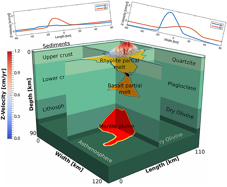
Figure 3. Result of the comparison between 2D and 3D models. Two cross sections are shown with their respective surface velocity in 2D or 3D. The velocity profile is very distinct, suggesting that 3D effects are important to take into account.

5.2. Gravity Anomaly Inversion

Before performing actual geodynamic simulations, we first derive a density structure of the magma reservoirs of the Yellowstone magmatic system, as gravity anomaly computations are much faster than geodynamic simulations. We implement the gravity computation as described in Turcotte and Schubert (2014). As comparison we use the compiled Bouguer anomaly data of DeNosaquo et al. (2009) (online archive of the Pan American Center for Earth and Environmental Sciences (PACES), shown in Figure 1), who performed a 2D inversion for the density structure. By varying the effective density of the two magma reservoirs, we invert for the 3D density structure. We vary the effective densities from 2340 kg/m³ to 2690 kg/m³ for the upper and from 2590 kg/m³ to 2730 kg/m³ for the lower reservoir, consistent with the effective density values resulting from the parametrization of Bottinga and Weill (1970) for the major elements found by Christiansen (2001), also shown in Table 1. Four end member cases are considered:

1. Grid search inversion: In this case, the gravity anomaly is fitted by varying the effective densities of the reservoirs as a whole, as shown in Figure 4A (data), Figure 4C (simulation result), Figure 4D (mapped misfit function), and Figure 4E (representative 2D cross section). Results show that we obtain an overall good fit to the data, with deviations of around 5-10 mGal (see Figure 4E). There is a trade-off between the two densities (Figure 4D). As expected, the gravity anomaly is more sensitive to the density of the shallower magma reservoir. The final result has a density of 2496 kg/m³ in the upper reservoir, and a density of 2,684 kg/m³ for the lower reservoir.

2. Heterogeneous magma reservoirs: We present a hand-made fit based on the result of the grid search inversion to the gravity anomaly in which we include smaller areas within the reservoirs that are allowed to have higher or lower densities. As starting point, the best fit from approach (1) was used. The result is shown in Figures 4B,E. In particular, a denser heterogeneity (slightly denser than the surrounding crust) within the north east part of the reservoir removed the anomalous perturbation in the gravity signal. Furthermore, the center of the magma reservoir was divided in a slightly denser part in the west and a less dense part in the east. As a result the misfit is reduced in some areas, and increases in others. Doing a better fit would potentially be possible if we allow for a full, laterally varying, density structure. Given the above-described non-uniqueness of the gravity problem it is however unclear whether this will give significant new insights in the dynamics of the system, while increasing the model parameters significantly.

3. Slightly larger reservoirs: Since the geometry is inspired by the seismic tomography data, which includes a regularization as part of the inversion, there is still significant room for interpretation regarding the reservoir size (which we constrained using the shape of the seismic velocity contour lines). To investigate this effect, we performed simulations with 10% larger reservoirs, which significantly overdetermines the gravity signal, shown in Figure 4E.

4. Slightly smaller reservoirs: Similarly, a reduction of the volume of the reservoirs by 10 %, while using the same density difference between reservoir and host rock, significantly underestimates the gravity signal, as shown in Figure 4E.

FIGURE 4

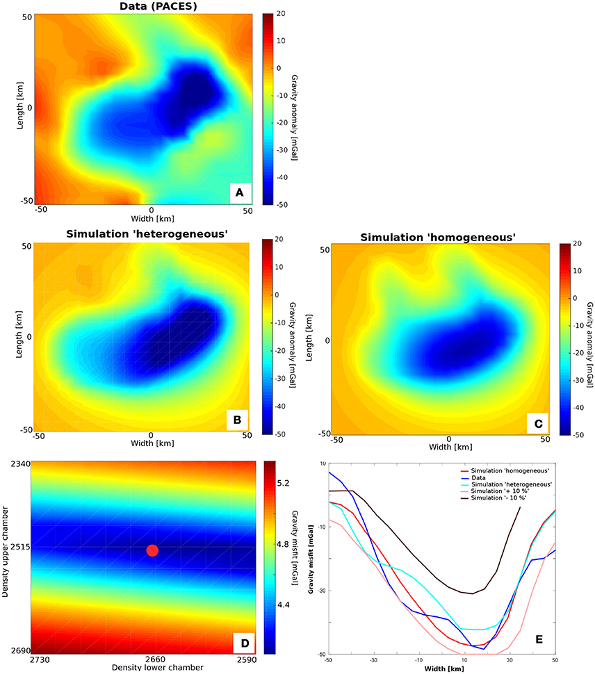
Figure 4. Result of the gravity inversion. (A) Observed gravity anomaly data from PACES. (B) Best manual fit assuming heterogeneous magma reservoir densities. (C) Best fit model by grid search inversion, keeping the density of the reservoirs homogeneous. (D) Misfit function in the grid search inversion. The color represents the least square misfit between the simulation and data, with blue colors indicating a good fit to the data. (E) Gravity anomaly comparison between simulation result and data at a representative 1D line across the surface (along length = 0 km).

Based on these results, we use the best-fit density structure of the grid search inversion in the remainder of this work. This assumes a density difference between upper reservoir and surrounding upper crust of around 100 kg/m³, independent of how this density difference is achieved. The density difference between the lower reservoir and lower crust has an approximately 3 times smaller effect on the gravity signal, as can be seen precisely in Figures 4D, 9C.

5.3. Forward Modeling

In the next step, we perform 3D visco-elasto-plastic compressible geodynamic simulations. Since we are mainly interested in the present-day deformation of the lithosphere, we need to run the simulations for a few time steps until stresses have elastically build-up and do not change significantly with time after which we evaluate the simulation (see Supplementary Material in Appendix 2 for additional details).

In our simulations, the long term surface uplift is driven by the buoyancy force, caused by the density difference between reservoirs and crust or plume and mantle, respectively, and is inverse proportional to the effective viscosity of the layers. In addition, magma pulses may further inflate a magma reservoir and induce a surface signal. We model this by either activating an overpressure lower boundary condition, or by a kinematic internal boundary condition, as explained later. Both conditions are activated only after a steady-state stress state has been achieved in the models, which is why these simulations take both the long-term geodynamic effects and the shorter-lived magmatic pulse into account. In the following, we discuss the impact of several end member simulations.

5.3.1. No Connections, Visco-Elastic

During phases of tectonic quietness, the magma reservoirs act as buoyant bodies emplaced in a elastically loaded crust. We tested this by performing a model with unconnected reservoirs and a visco-elastic crust without taking plasticity (generation of faults or weak zones in the crust) into account. Maximum surface velocities are on the order of 0.2 cm/year, shown in Figure 5A. Furthermore, significant deviatoric stress occur between the reservoirs of up to 120 MPa, which suggests that it is likely that brittle failure would actually occur in these places and connect the reservoirs.

FIGURE 5

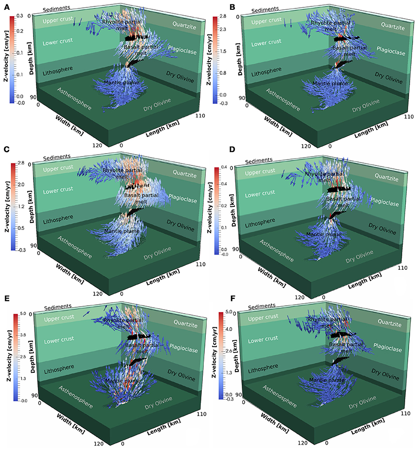
Figure 5. Summary of the velocity structure of different end member simulations. (A) No connection between the reservoirs and no plasticity. Maximum vertical velocities at the surface are 0.2 cm/year. Black parts show the connection between the reservoirs which is set to the surrounding crustal viscosities in case they are inactive. (B) Connections between the reservoirs and no plasticity. Maximum vertical velocities at the surface are 0.8 cm/year. (C) Connections between the reservoirs and plasticity. Maximum vertical velocities at the surface are 1.2 cm/year. (D) Connections between the reservoirs, plasticity and a higher viscosity of the reservoirs of 10²¹ Pa s, implying a lower melt content. The maximum vertical velocity at the surface is 0.2 cm/year. (E) Case with slightly larger connections between the reservoirs, plasticity and a basal boundary overpressure of 50 MPa. Maximum vertical velocity at the surface is 2.4 cm/year. (F) Case with a prescribed kinematic boundary condition between the reservoirs to simulate influx from the middle to the upper reservoir of around 8 cm/year. Maximum vertical velocity at the surface is 2 cm/year. The downwards center of the reservoir is moving upwards which must result in a (low magnitude) downwards movement of material elsewhere.

5.3.2. Connections, Visco-Elastic

In a next test, we therefore inserted a connection between the reservoirs in the models (as shown in Figure 5B). This increased the maximum surface uplift velocities of up to 0.8 cm/year, which is consistent with the lower bound of the observed uplift velocities in Yellowstone, recorded during phases of low activity (e.g., Chang et al., 2007, 2010; Vasco et al., 2007).

5.3.3. Connections, Visco-Elasto-Plastic

The crust above large scale volcanic systems is faulted in many places (e.g., Reid, 2004). For rocks, a first order representation of the stress at which they yield is given by Byerlee's law which can be numerically mimicked by a Drucker-Prager frictional plasticity law (Drucker and Prager, 1952). Numerical simulations that implement this will limit the stresses to remain below or at the yield stress. To understand the effect of this on the large-scale dynamics of the system we performed a simulation in which plasticity was activated (with a friction angle of 30°, and a cohesion of 1 MPa). The results show that plastic yielding is predominantly active above the magma reservoirs. As it effectively weakens the crust, it results in higher surface velocities of up to 1.2 cm/year (Figure 5C). To give a better feeling of the overall velocity field within the system we created a movie consisting of passively advected markers. The movie is given in the online supplement and is described in Supplementary Material in Appendix 4.

5.3.4. Connections, Visco-Elasto-Plastic, Sill-Type Body

The presently most common view of magmatic systems is that they are not composed of homogenized, partially molten bodies, but rather of sill complexes Cashman et al. (2017). As such the assumption that we made before, of having magmatic bodies with a constant density and viscosity, may be an oversimplified representation of volcanic systems such as the Toba caldera as proposed by Jaxybulatov et al. (2014). To test the effect of a sill-like, rather than a homogeneous, magma body we cut the two upper magma reservoirs by layers of the representative crust. This leads to sill like structures of partially molten layers with a height of about 4 km that alternate with colder crustal layers that are roughly 2 km high. A simulation with unconnected sill bodies and without a connection to the mantle plume results in a maximum surface velocity of 0.3 cm/year, comparable to the unconnected case discussed in section 5.3.1. Connecting the sill bodies internally and adding a connection to the mantle plume increased the surface velocity to 1 cm/year. The endmember with connections is shown in Supplementary Material in Appendix 5.

5.3.5. Connections, Visco-Elasto-Plastic, Less Melt

So far, our models considered the partially molten viscous reservoirs to have a uniform and low viscosity of 10¹⁹ Pa s, which implies that the melt content is sufficiently large to weaken the effective viscosity of the reservoirs to this amount (from an effective solid rock viscosity of 10²³−10²⁴ Pa s). Yet, seismic tomography results suggests that the melt fraction in the upper reservoir may be no more than 10% and even less in the deeper reservoir (Huang et al., 2015). Whereas it is unclear how robust these findings are, given the km-scale wavelength of seismic waves and the dampening used in seismic tomography inversions, it is at least feasible that the effective viscosity is larger than we assumed. We therefore performed an additional simulation in which the viscosity of the magma reservoirs was increased by two orders of magnitudes. Results show that this reduces the maximum surface velocities by a factor 6, from 1.2 to 0.2 cm/year (Figures 5D, 9D). This suggests that the viscosity of the reservoirs does play an important role for the surface velocities, and that this is not solely affected by the rheology of the host rocks.

5.3.6. Connections, Visco-Elasto-Plastic, Mantle Influx

In volcanology, uplift rates of volcanoes are often interpreted by comparing them with predictions of analytical or numerical models that consider a (spherical) magma reservoir that is emplaced at a given depth and has a certain amount of overpressure applied at its boundary. Physically, this approach mimics the inflation of a magma reservoir after the addition of a new batch of magma, and if this magma reservoir is embedded in a compressible elastic host rock, it will deform both the host rocks and the free surface (e.g., Battaglia and Segall, 2004; Gerbault et al., 2012). In numerical codes, this is typically done by treating the magma reservoir itself as a boundary condition, which can be benchmarked vs. the elastic Mogi solution (Mogi, 1958) or a visco-elastic variation of it (Del Negro et al., 2009). Whereas this approach is certainly applicable to address deformation within the shallow crust beneath a volcano, there are a number of problems of employing it to the whole lithosphere. The first issue is related to where the magma pulse comes from. In Yellowstone, magma in the upper reservoir may either come from the mantle plume (an influx condition in our setup), or from extraction of melt from the lower reservoir, which would result in both inflation in the upper crust and deflation in the lower crust. We consider both scenarios.

The first scenario assumes that additional magma in the upper crust comes from a new pulse of magma in the asthenosphere. The usual way of implementing this in numerical models, by setting an internal pressure boundary condition, has the disadvantage of eliminating the background lithospheric uplift rate, caused by the density difference between the magma reservoir and the host rocks. This thus implies that such models only consider the effect of overpressure on deformation. An alternative approach, which we follow here, is to apply an overpressure condition at the lower boundary of the model, which propagates through the system and causes an inflation of the upper reservoir, as long as it is connected to the lower boundary through weak zones. This has the advantage that it mimics more closely what happens in nature and allows for more complex partially molten regions, while at the same time taking the buoyancy effect of the reservoirs into account. To test whether this approach works, we benchmarked our implementation with the Del Negro viscoelastic benchmark (Supplementary Material in Appendix 3).

To test the effect of mantle magma influx on the Yellowstone model configuration, we applied an additional constant overpressure of 50 MPa at the intersection between the mantle plume and the lower boundary. Results show that this significantly increases the velocities within the mantle plume, while only resulting in slightly larger surface velocities (Figure 5E). The effectiveness with which the overpressure influences the surface velocity scales with the size of the weak connection zones between the reservoirs. Small connections result in a significant increases of the velocity field within the mantle plume, of which only a small amount is transferred to the surface. Increasing the size of the connections increases the surface uplift velocity, which can go up to 2.4 cm/year for large connection zones (see Figure 9E).

An additional advantage of our implementation is that it allows recomputing the effect of the overpressure in terms of an influx or an inflation volume. One can compute the influx volume by multiplying the boundary velocity, resulting from applying the overpressure, by the timespan of the inflation, or the timespan of high surface uplift velocities and retrieve the amount of added volume of magma to the system. The area of applied overpressure in all simulations is 50 km². If one assumes an overpressure of 50 MPa, resulting in an average z-velocity of 23.4 cm/year at the boundary (approximately 3 cm/year within the plume), and timespan of high activity described by Chang et al. (2010) from 2003 to 2008 the magma inflation volume is 0.06 km³ at the mantle plume level after only 5 years.

5.3.7. Connections, Visco-Elasto-Plastic, Influx Reservoirs

The second scenario to add magma into the upper crustal reservoir, is by taking it from partial melting or fractional crystallization of the lower crustal magma reservoir. This implies that inflation in the upper magma reservoir is accompanied by deflation in the lower reservoir, which can be implemented numerically by introducing a connecting zone ('dike') between the two reservoirs in which a Poiseuille-flow (quadratic) velocity field is prescribed as an internal boundary condition. By varying the magnitude of the velocity we can control both the mass flux and the pressure gradient between the reservoirs. If only a connecting dike zone is present, the self consistent (buoyant) velocity in the channel has an average value of 4.3 cm/year, which is equal to moving a volume of 0.006 km³ between the reservoirs within 5 years. If we increase this velocity to an average of 8 cm/year, the surface velocities increase from 1.2 to 2 cm/year and the inflation volume to 0.012 km³ (Figure 5F). The volume of the applied velocity is 50 km³ and the cross sectional area is 30 km². This thus has the largest impact on the surface velocities of all the scenarios we considered (see Figure 9F for a summary).

5.4. Stress Directions

Our models also compute stress orientations, which can be compared against available observations. In Yellowstone, Waite and Smith (2004) assembled the local stress orientation of the minimum principal stress σ₃ for selected locations by using earthquake focal mechanisms (white arrows in Figure 1). Comparing modeled with observed principal stress directions reveals that there is a good agreement, particularly with respect to the stress orientation that changes from West-East to North-South (Figure 6). Furthermore, both the connected and unconnected geometries have almost the same patterns, suggesting that both scenarios correlate well with the data.

FIGURE 6

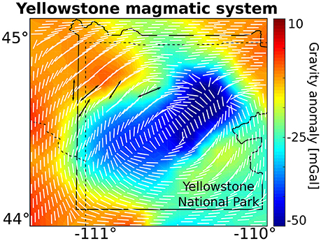
Figure 6. Orientation of the minimum principal stress. Black arrows represent the orientation of the minimum principal stress taken from Waite and Smith (2004) and references therein. White arrows show the result of the simulation with no connection between the reservoirs, while grey arrows show the result of the simulation with connected reservoirs and a mantle plume (Figure 5C). The stress orientation is computed at the surface. Results reproduce the rotation of the stress field from West-East to North-South. Furthermore, the connected vs. the unconnected case do not show significant differences.

5.5. Parameter Sensitivity

So far, we focused on how the connectivity between the reservoirs, the type of rheology and the inflation affect the surface velocity. However, in addition, material parameters such as the powerlaw exponent or the density will affect the dynamics of the system. We therefore perform a parameter sensitivity analysis, shown in Figure 7, to determine the model parameters that play a key role in controlling the surface velocity. We compute these sensitivities for the representative simulation with visco-elasto-plastic rheology and connected reservoirs. Results are obtained for the cases in which we take the activation energy, the power law exponent and the density of the reservoirs into account, which amounts to 16 parameters in total. Of these, the viscosity parameters of the lower crust, as well as the density of the upper crust, are the most important parameters as can be seen in Figure 7. The size of the spheres in the figure visualize the normalized relative importance of the parameters. To enable direct comparison, each parameter type, e.g., activation energies, is normalized over the maximum parameter value within the type.

FIGURE 7

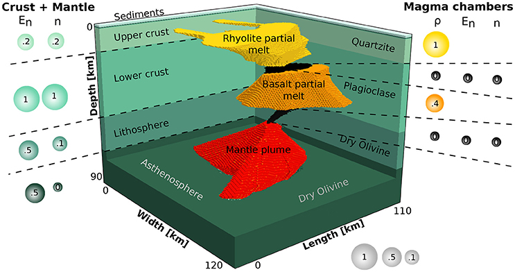
Figure 7. Result of the adjoint parameter sensitivity study. The size of the sphere represents the relative importance of the parameter in affecting the surface velocity above the uppermost magma reservoir. Every physical parameter is normalized by its value for each rock phase (e.g., the activation energies of all phases are normalized with respect to each other). The viscosity of the lower crust, lithosphere and the lower crustal magma reservoir together with the densities of the magma reservoirs are the key model parameters.

5.6. Adjoint Inversion

In the next step we solve an inverse problem based on our “best-scenario” model from previous section to obtain an improved fit between the simulations and observed GPS velocities. We allow the inversion to vary the activation energy and the power law exponent of the upper and lower crust, the asthenosphere and lithosphere. Figure 8A shows the viscosity field, which was used as initial guess. The final viscosity field has a significantly weakened crust as a result of an increased power law exponent of the upper crust from 2.4 to 3 and from 3.2 to 4.6 for the lower crust (Figure 8B). The inverse problem is solved by a steepest descent method and typically demonstrates a quick convergence, facilitated by a robust line-search algorithm (Figure 8E).

FIGURE 8

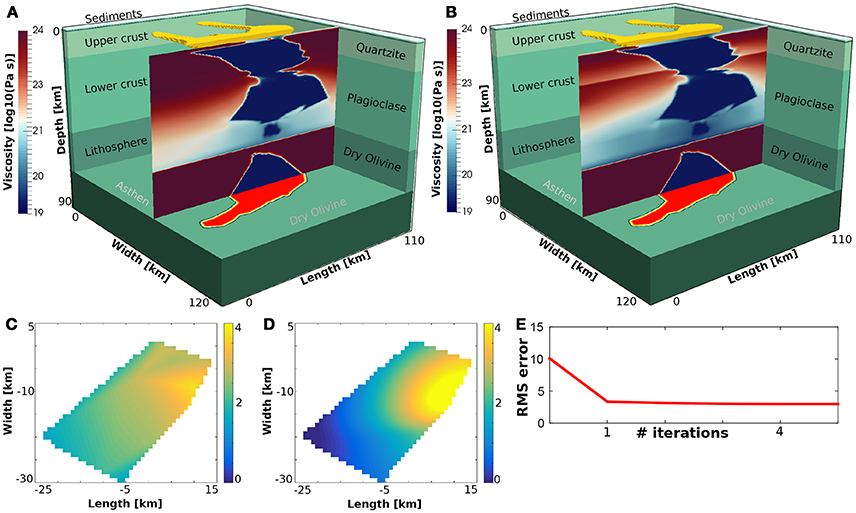
Figure 8. Summary of the adjoint inversions for material parameters. (A) Initial viscosity field of the visco-elasto-plastic connected case was (Figure 5C) used as starting guess for the inversion. (B) Final viscosity field after converged iterations, showing a significantly weakened crust by increasing the powerlaw exponents of the crust. (C) Map view of interpolated surface uplift from Chang et al. (2010) during the period of September 2007–September 2008, which is used as data for our inversions. (D) Map view of the vertical surface velocity field after converged iterations. Both the patterns and magnitude are similar, even though the numerical model has lower velocities toward the boundaries of the map, perhaps caused by crustal heterogeneities that were not taken into account in the models. (E) Cost function as root mean square of vertical surface velocity vs. number of iterations. Due to a good initial guess and robust line search acceleration, convergence is achieved quickly.

A comparison between the modeled and observed velocity field between September 2007 and September 2008 (interpolated from data from Chang et al., 2010), shows that the pattern and magnitude are similar (Figures 8C,D). This suggests that it is possible to fit the long-term or background surface velocities above magmatic systems by changing the viscosity structure of the crust. Lowering the viscosity allows for larger displacements in a shorter amount of time, that are triggered by the density difference, resulting in higher velocities. Smaller-scale differences that can be observed toward the boundaries, may occur because we consider the rheology of the crust to be homogeneous outside the magma reservoirs, whereas in nature weakening of the nearby surrounding crust may result from phases of inflation, heating, or deflation. In general, changing the viscosity structure only influences the long term surface velocities and stresses, and does not represent a short term signal like the inflation models discussed in section 5.3.6.

6. Discussion

Our results imply that buoyancy driven uplift for large magma reservoirs at large magmatic systems such as Yellowstone is active on a long term scale (thousands of years) with small rates. The rate itself strongly depends on the connectivity between the reservoirs or sills within the magmatic system. If the magma bodies are only connected sporadically, the background uplift signal will be even smaller since the buoyancy effect from deeper reservoirs becomes negligible. The strength of this effect is further limited by the viscosity of the surrounding material and by the viscosity of the magma bodies. Thus, a larger amount of partial melt would decrease the viscosity of the magma bodies and would result in higher uplift rates. In order to show the difference between the long-term and more short-term processes we conclude that the effect of magma injection on the surface uplift can be much higher than the long term buoyancy signal. Even small amounts of injected magma at the level of the mantle plume can be recorded at the surface. However, effects such as volatile degassing were not taken into account in this study which may result in changes in the dynamics of a magmatic system on a very short time scale (Vargas et al., 2017). Other effects, that could potentially play an important role, and should ultimately be considered in these type of models, are: (i) deformation of a two- or three-phase mush, (ii) volume changes resulting from crystallization and melting (Fournier, 1989), (iii) the effect of volatiles in the viscous formulation of the partially molten rocks. In addition, we can potentially increase the robustness of the inversions by taking more data into account, such as seismic activity as an estimation for the proximity to failure within the crust, or by directly inverting for stress orientations as well. Furthermore, instead of inverting for the direct parameters viscosity and density one could invert for a parameter that couples the effective material parameters in magmatic systems, such as temperature or melt fraction.

Seismic observations may not be sufficient to precisely constrain the volume of a reservoir, furthermore the possible interpretations on the dynamics of the reservoir are still debated. For such problems it is helpful to include results from numerical simulations as presented in this work. Taking the seismic observations as initial guess for the shape and sizes of the reservoirs and then inverting for the material parameters based on the misfit between the mechanical result and the measured surface velocities (GPS or InSAR) can shed additional light on the dynamics of the reservoir and can help constraining effective parameters of viscosity and density more precisely. From these effective quantities one could, by taking area specific thermodynamic data into, recompute melt fractions. Furthermore, geodynamic simulations can easily test different volumes (within the uncertainty of the seismic observations) and quantify the difference in the effective parameters, and provide uncertainties on these parameters. One example presented, shows that a reduction of the reservoir volume by 10% reduces the gravity signal by about 30 %. As such a density that is 10% higher should fit the gravity signal sufficiently well. This can further be explained by a different volume of melt fraction, a lower solid rock density (possibly due to a high temperature) or possibly a sill like body which cannot be resolved by seismic imaging techniques due to wavelengths of several kilometers in size. If one, as mentioned above, couples the reservoir parameters, such as density and viscosity, to one key parameter such as temperature, one should be able to uniquely retrieve a volume of the reservoir that is consistent with observations at the surface. The uniqueness of this parameter combination can be supported y including additional data into the inversion, such as stresses orientations at depth.

This method can be applied in the future to any well monitored volcanic system such as the Phlegrean Fields (caldera system) or Etna (no caldera system) where it can help constraining which of the mechanical processes—viscous, elastic or plastic—are active and have a key influence the surface observations. It can further help to estimate the long term background stress state around the magmatic system, which can potentially be incorporated as boundary conditions into smaller scale numerical models focussing on part of the system. With our approach we can easily incorporate complex 3D structures and retrieve more complex surface responses than previous approaches (like the traditionally applied Mogi source). In case 4D seismic observations are available, there is the possibility to invert for the different stages of the seismic observations, and determine how the volumes and effective parameters at each stage of the seismic observation changed with time. It would be interesting to apply this approach to other, geophysically well-studied, magmatic systems.

7. Summary and Conclusions

In this work, we present 3D visco-elasto-plastic numerical modeling of the lithospheric scale Yellowstone magmatic system. The geometry of our models is inspired by the recent seismic study of the area described in Huang et al. (2015). Additionally, the effective densities of the magma host rocks and the crust are obtained by thermodynamically consistent modeling using Perple_X (Connolly, 2009) and the approach in Bottinga and Weill (1970).

In a first step, we show that it is important to consider 3D models rather than 2D ones, because the magnitudes (e.g., of velocities) can be very different. Next, we used gravity inversions to derive a reasonable density structure, which was subsequently used in a series of forward simulations in which we tested the effect of lithospheric rheology, reservoir connectivity and magma influx on surface velocities. These simulations suggest that observed background uplift rates can be obtained for simulations in which the reservoirs are connected and plasticity is active in the upper crust surrounding the magma reservoirs. Velocity magnitudes obtained in this manner vary between 0.2 and 1.2 cm/year depending on whether plasticity is active or not, on the viscosity of the reservoirs, and on whether the reservoirs are connected, as shown in Figures 9A,B.

FIGURE 9

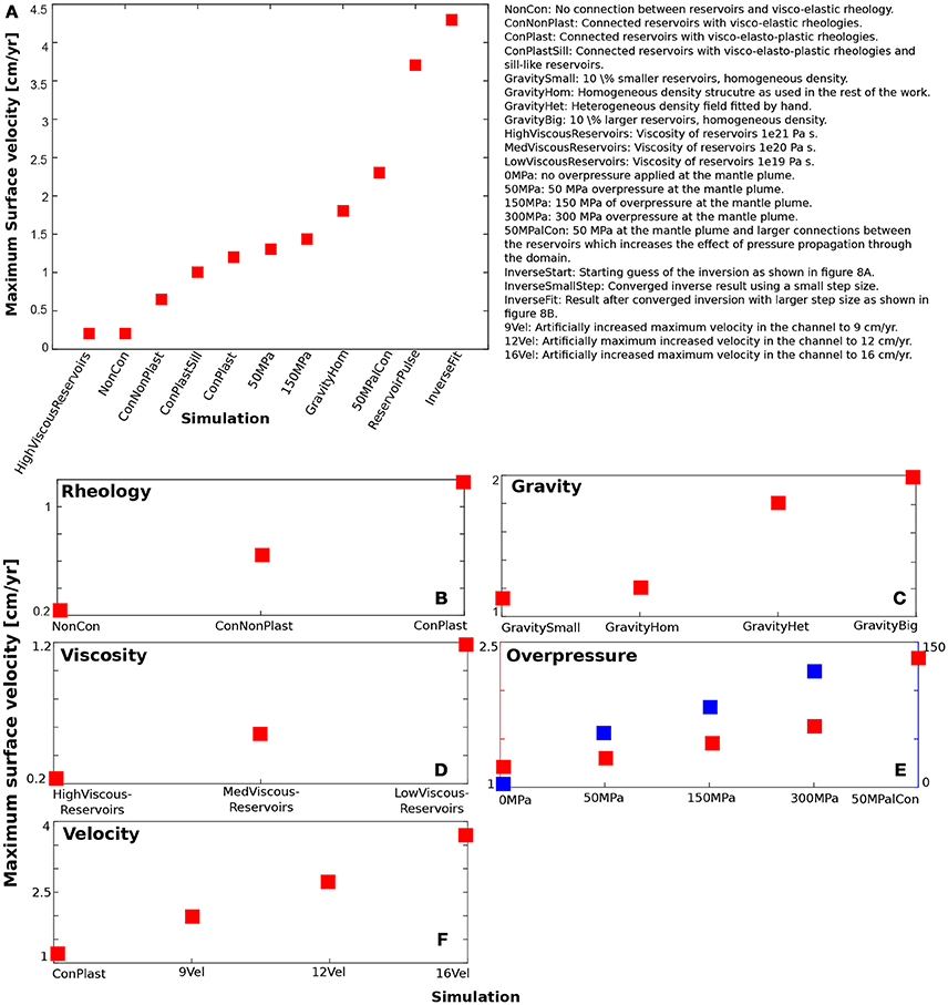
Figure 9. Summary of the impact of the various parameters considered here on the vertical surface velocity. (A) Set of representative simulations and the resulting surface velocities. (B) Effect of rheology. (C) Effect of the different density models on the surface velocity. (D) Viscosity of the magma reservoirs. (E) Effect of overpressure at the mantle plume. Red squares represent the surface velocity. Blue squares show the maximum z-velocity at the boundary where the overpressure is applied (numbers on the right axis). (F) Effect of kinematic internal boundary condition between the reservoirs simulating inflation and deflation between the upper and lower reservoirs, respectively. The largest effect on the vertical surface velocity is caused by changing the kinematic boundary condition.

We perform a comparison of the surface velocities with GPS measurements. Chang et al. (2010) report phases of higher surface uplift rates during a timespan of 1 year between September 2007 and September 2008, representing velocities between 2 and 4 cm/year. To account for these enhanced velocities we considered two additional processes: (i) overpressure at the lower boundary of the domain to simulate magma rising from the mantle plume through the magmatic plumbing system, and (ii) magma transfer from the lower to the upper magma reservoir, by applying a kinematic internal boundary condition between the two reservoirs at the location of the connection. The effect of overpressure appears to have a relatively minor impact on the surface velocities and most likely only contributes to the long term signal at the surface velocities. On the other hand, the prescribed Poiseuille flow between the upper and lower reservoirs has a much bigger effect. Increasing the magma flux between the reservoirs results in large changes of the surface velocities, e.g., 12 cm/year imposed velocity within the connection, which is equivalent to an inflation volume of 0.018 km³ within only 5 years, nearly doubles the surface uplift velocity to 2.6 cm/year.

An adjoint-based sensitivity analysis is performed to demonstrate that the viscosity parameters of the upper and lower crust are of key importance for the surface velocities. An inversion was performed to better fit the models to both the magnitude and spatial pattern of the recorded uplift during a period of high activity with velocities of up to 4 cm/year (Chang et al., 2010). Results show that this can be fitted with a weakened crust. Yet, changing the viscosity structure of the whole crust affects the long term uplift signal as well, while a short term period of enhanced uplift is more likely caused by a smaller scale magmatic pulse in the upper crust. In future work, it would thus be interesting to take the temporal evolution of the surface uplift signal into account (for example from INSAR data) as it may allow unraveling both the long term uplift, and the emplacement of a smaller scale magma pulses in a rheologically realistic lithosphere.

Author Contributions

GR created the manuscript, created the Perple_X phase diagrams, temporarily implemented the gravity computation and the phase diagram feedback into LaMEM and performed all simulations presented in this work. BK proposed the main idea and helped in all aspects of this work. AP is the main developer of LaMEM and helped with implementation issues. TB supported processing the raw gravity data, implementing the gravity solver into LaMEM and helped with interpreting inversion results. All authors contributed to the writing and statements made in this work.

Funding

GR received funding from the University of Mainz.

Conflict of Interest Statement

The authors declare that the research was conducted in the absence of any commercial or financial relationships that could be construed as a potential conflict of interest.

Acknowledgments

Parts of this research were conducted using the supercomputer Mogon and/or advisory services offered by Johannes Gutenberg University Mainz (https://hpc.uni-mainz.de/), which is a member of the AHRP (Alliance for High Performance Computing in Rhineland Palatinate, www.ahrp.info) and the Gauss Alliance e.V. The authors gratefully acknowledge the computing time granted on the supercomputer MOGON I and MOGON II at Johannes Gutenberg University Mainz (https://hpc.uni-mainz.de/).

Supplementary Material

The Supplementary Material for this article can be found online at: https://www.frontiersin.org/articles/10.3389/feart.2018.00117/full#supplementary-material

References

Angiboust, S., Wolf, S., Burov, E., Agard, P., and Yamato, P. (2012). Effect of fluid circulation on subduction interface tectonic processes: Insights from thermo-mechanical numerical modelling. Earth Planet. Sci. Lett. 357, 238–248. doi: 10.1016/j.epsl.2012.09.012

ORIGINAL RESEARCH article

Unraveling the Physics of the Yellowstone Magmatic System Using Geodynamic Simulations

1. Introduction

2. Methods

2.1. Physics and Numerics

2.2. Adjoint Equations

2.3. Thermodynamic Modeling

3. Model Setup and Data Integration

4. Inverse Modeling Approach

5. Results

5.1. 2D vs. 3D

5.2. Gravity Anomaly Inversion

5.3. Forward Modeling

5.3.1. No Connections, Visco-Elastic

5.3.2. Connections, Visco-Elastic

5.3.3. Connections, Visco-Elasto-Plastic

5.3.4. Connections, Visco-Elasto-Plastic, Sill-Type Body

5.3.5. Connections, Visco-Elasto-Plastic, Less Melt

5.3.6. Connections, Visco-Elasto-Plastic, Mantle Influx

5.3.7. Connections, Visco-Elasto-Plastic, Influx Reservoirs

5.4. Stress Directions

5.5. Parameter Sensitivity

5.6. Adjoint Inversion

6. Discussion

7. Summary and Conclusions

Author Contributions

Funding

Conflict of Interest Statement

Acknowledgments

Supplementary Material

References

This article is part of the Research Topic

People also looked at