Short-Term Magnetic Field Variations From the Post-depositional Remanence of Lake Sediments

Introduction

Sediments record geomagnetic field variations through acquisition of a detrital remanent magnetization (DRM). Measurements of the acquired magnetization, i.e., paleomagnetic data, contain information about past geomagnetic field behavior on a range of time scales. Geomagnetic field models constructed from sedimentary paleomagnetic data and remanent magnetizations obtained from archeological artifacts and lava flows (hereafter referred to as archeomagnetic data) provide a global picture of the geomagnetic field and its evolution both at Earth's surface and at the core-mantle boundary (Korte et al., 2009, 2011; Licht et al., 2013; Nilsson et al., 2014). The superior geographical distribution offered by sedimentary paleomagnetic data compared to archeomagnetic data make sedimentary records essential for such global field reconstructions. Another advantage of sedimentary data is that they normally yield continuous records, often encompassing most of the Holocene, as opposed to archeomagnetic data that provide spot readings concentrated within the last 2000 years. Stratigraphic control in a sediment core also enables construction of precise age-depth models (e.g., Bronk Ramsey, 2009; Blaauw and Christen, 2011) using a variety of dating techniques. For example, varve counting can potentially provide annual resolution (e.g., Stanton et al., 2010; Striberger et al., 2011; Mellström et al., 2013).

Whilst sedimentary paleomagnetic data are useful, potential effects of post-depositional remanent magnetizations (pDRM) that can lead to both delay and smoothing of the recorded geomagnetic signal (e.g., Roberts and Winklhofer, 2004), present huge challenges for their application in geomagnetic field modeling and dating. The classical pDRM concept describes a process where the magnetization is acquired gradually as sediments compact until magnetic particles cannot further align with the geomagnetic field and become locked into place by the sediment matrix (Irving and Major, 1964; Kent, 1973; Hamano, 1980; Otofuji and Sasajima, 1981). This process has been described by so-called “lock-in” functions, which model the fraction of pDRM acquired as a function of depth below the surface or the mixed layer (e.g., Meynadier and Valet, 1996; Channell and Guyodo, 2004; Roberts and Winklhofer, 2004; Suganuma et al., 2011; Roberts et al., 2013a). Other efforts have questioned this classical pDRM acquisition concept arguing that flocculation of sediments prevents substantial post-depositional movement of grains within pore spaces (Katari et al., 2000). Alternative sediment mixing models have instead demonstrated the potential role of bioturbation in pDRM acquisition (Mao et al., 2014; Egli and Zhao, 2015). In addition, the presence of magnetotactic bacteria either living at the sediment/water interface or in the sediments, giving rise to either bio-depositional or bio-geochemical magnetizations, is becoming more recognized (e.g., Tarduno et al., 1998; Heslop et al., 2013; Roberts et al., 2013b; Larrasoaña et al., 2014; Mao et al., 2014). Despite uncertainties regarding the processes involved, there is mounting empirical evidence for natural remanent magnetization (NRM) acquisition at depths >10 cm below the sediment/water interface (Lund and Keigwin, 1994; Sagnotti et al., 2005; Suganuma et al., 2011; Mellström et al., 2015; Simon et al., 2018). These processes, hereby collectively referred to as lock-in, all act as a natural smoothing filter that produces a time lag between the age of the magnetization and the time of deposition of the sediments carrying the magnetization. This attenuation of high frequency geomagnetic field variations limits the possible resolution of paleomagnetic data, which depending on accumulation rates could mean effective resolutions on the order of 100–1000 years, which reduces the information content of the record (Roberts and Winklhofer, 2004).

Understanding the nature of lock-in is critical if geomagnetic field models, which rely increasingly on sedimentary data as models are extended back in time, are to reproduce higher frequency (centennial or even decadal) field variations. Nilsson et al. (2014) showed that the independent ages of sedimentary paleosecular variation (PSV) data used to constrain the global pfm9k.1a geomagnetic field model are systematically older than model predictions. This is particularly apparent over the past 3000 years where the model is more heavily constrained by archeomagnetic data, which suggests that post-depositional lock-in might be a widespread phenomena in lake/marine sediments all over the world.

So far, investigations of pDRM effects in ancient sediments have required high-precision chronologies to be able to distinguish between lock-in delay and dating uncertainties. Mellström et al. (2015) were able to obtain such high-precision chronologies (uncertainties of ±20 years, 95% confidence) spanning the period between 3000 and 2000 years BP using the ¹⁴C wiggle-match dating technique in two Swedish lake sediment records (Gyltigesjön and Kälksjön). By comparing PSV data from these records with archeomagnetic field model predictions that are not affected by post-depositional smoothing and delay, they investigated and evaluated the suitability of a range of lock-in filter functions proposed in the literature. Application of this approach is, however, limited by the high costs involved (15 and 19 radiocarbon dates used, respectively) and special conditions of having floating varve chronologies that provide roughly annual resolution between each ¹⁴C date.

Here we present a new Bayesian method to simultaneously model lock-in delay and construct an age-depth model based on paleomagnetic data and archeomagnetic field model predictions. As well as being the first paleomagnetic method that addresses problems related to pDRM acquisition in age-depth modeling, the method provides key insights into pDRM acquisition. Most importantly, it is able to recover high frequency field variations that are lacking in Holocene field models (Nilsson et al., 2014). To illustrate these applications of our new method, we use the two Swedish lake sediment records, Gyltigesjön (Snowball et al., 2013) and Kälksjön (Stanton et al., 2010, 2011), as case studies.

Methods

Our new Bayesian method models simultaneously lock-in and constructs an age-depth model based on paleomagnetic data. Details of the method are provided in the Supplementary Information. The age-depth model is built on the widely used “Bacon” dating software of Blaauw and Christen (2011) to combine both radiocarbon and paleomagnetic measurements. It is based on controlling sediment accumulation rates using an autoregressive gamma process. Radiocarbon age determinations R_j taken along the sediment core at depth z_j provide tie points to which the age-depth model can be fitted.

Paleomagnetic Data

Paleomagnetic measurements, inclination I_i and declination D_i, taken at depth z_i can be used indirectly to constrain the age-depth model through correlation to a reference curve with known ages. Here we chose to include only paleomagnetic field directions and not relative paleointensity estimates, which are usually associated with larger and more poorly defined uncertainties.

Sedimentary Paleomagnetic Data Uncertainties

Uncertainties in sedimentary paleomagnetic directional data can be difficult to assess. The experimental error, e.g., the maximum angular deviation (MAD, see Kirschvink, 1980), typically only accounts for a fraction of the total error budget. Other potential sources of error include: (i) compaction leading to some degree of inclination flattening (Blow and Hamilton, 1978; Anson and Kodama, 1987), (ii) chemical and physical overprinting (Snowball and Thompson, 1990), (iii) compression and extension of sediments caused by coring equipment (Bowles, 2007) and sub sampling into u-channels or boxes (Gravenor et al., 1984). In addition, potential problems with core orientation and unwanted and unknown core rotation, which affects declination data, will also add to the error budget. Traditionally, the total error is estimated by smoothing data and calculating the dispersion of paleomagnetic directions over the selected range of depths/ages, preferentially from several independently oriented cores. This method has an obvious disadvantage for our analyses that it introduces additional data smoothing, which is not related to lock-in processes (Mellström et al., 2015). The error estimated using this approach could also underestimate data uncertainties severely if the record is only based on one core, which is often the case for Holocene paleomagnetic data.

To avoid binning or smoothing of data we use data at sample level. To account for experimental error, we convert the MAD into an α₉₅ angle, following Khokhlov and Hulot (2016), which in turn can be expressed as an α₆₃ angle, the Fisher (1953) distribution equivalent of a standard error, using:

To account for uncertainties related to coring and subsampling etc., we introduce an additional orientation error, which is added in quadrature to the α₆₃. Based on Stanton et al. (2011), who measured the tilt of core penetration based on the angle of sediment laminations, we use an orientation error of 2°. This additional error effectively limits the measurement precision to ±2° but does not account for potential systematic errors, e.g., induced by core rotation. To minimize the influence of such systematic errors, both inclination and declination data are treated as relative values and adjusted so that the mean inclination (declination) matches the mean reference inclination (declination) determined over the same depths. Inclination and declination data are affected by different sources of uncertainty and are therefore treated independently. The inclination error is derived directly from the α₆₃ angle (σ_I = α₆₃) and the declination error, which depends on inclination, is determined as follows:

Geomagnetic Field Reference Curve

To constrain an age-depth model, paleomagnetic data are correlated to a geomagnetic reference curve with “known” ages. Such reference time series, B(t), are readily obtained from geomagnetic field model predictions for the site coordinates. Geomagnetic field model predictions frequently also come with some form of uncertainty estimates, σ_B(t), usually based on bootstrap sampling of the paleo/archeomagnetic data (Korte et al., 2009).

A range of both regional and global geomagnetic field models are available and the choice of which model to use largely depends on the age range under investigation. To account for potential lock-in effects in sediments, the choice of model is restricted to those based exclusively on archeomagnetic data to ensure that they are not affected by lock-in processes. This includes measurements on archeological artifacts and igneous rocks but not on lake or marine sediments. There are many archeomagnetic models from which to choose (e.g., Korte et al., 2009; Licht et al., 2013; Pavón-Carrasco et al., 2014) and as shown by Mellström et al. (2015), the choice of model has some implications for the results. Data limitations restrict the effective range of these models, and consequently application of the dating method, to the past 3–4 millennia.

The number of paleomagnetic data points used in our analyses must remain constant for all investigated age-depth models. This means that the ages associated with a paleomagnetic measurement are restricted to the age range of the geomagnetic field model used. We, therefore, introduce a paleomagnetic depth limit z_lim, below which paleomagnetic measurements are discarded.

Outliers

The total error budget for a given paleomagnetic measurement, as outlined above, will account reasonably for errors arising from sampling and measurements as well as the model uncertainty, but some data may still have much greater dispersion. To account for the possibility of such outlying data, we follow a suggestion of Sivia (1996) who derived an expression for the likelihood of normally distributed data with uncertain error estimates (Figure 1). Take measurement y with an expectation μ and estimated uncertainty ω. We assume that the true uncertainty (ς) is greater or equal to our estimate (ω) and assign the prior distribution $\frac{\omega }{{\varsigma }^2}$, for ς ≥ ω. The unknown parameter, ς, is then marginalized to obtain the following likelihood:

where ${\chi }^2=\frac{{(y-\mu )}^2}{{\omega }^2}$. Although this form is only strictly valid for normally distributed (rather than spherically distributed) data, in the scheme used here declination and inclination are treated separately, and are assumed to be approximately normally distributed.

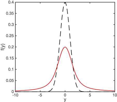
Figure 1. Standard Gaussian probability distribution with zero mean and standard deviation of one (dashed black) and the derived likelihood distribution (solid red) as described in the text.

Lock-In Modeling

The lock-in process is modeled following Roberts and Winklhofer (2004). First the geomagnetic field input time-series, B(t), is converted to a depth-series, B(z), using a given age-depth model (see Supplementary Information). A pDRM lock-in filter function, (z′) (Figure 2, see below for details), describes the relative contribution of layer to z′ the total pDRM acquired at each depth (z) down to a depth λ below the sediment/water interface, such that:

where P(z) is the pDRM obtained by convolving the geomagnetic field depth-series. The primed coordinates refer to the depth during deposition and the unprimed coordinates represent the actual depth of the recovered sediments (compaction during burial is not taken into account). The z′ variable takes values from 0, at the start of deposition of a sediment horizon, to λ as this horizon is progressively buried. The presence of a bioturbated or mixed layer is not taken into account in the model because this is not relevant to our case studies, where both records consist of undisturbed varved sediments (Mellström et al., 2015).

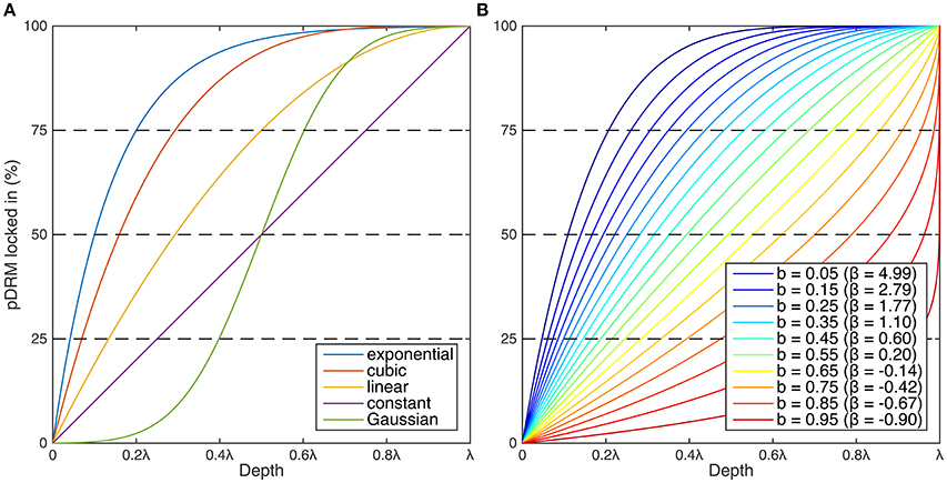
Figure 2. Illustration of (A) five lock-in functions from the literature (constant, Gaussian, linear, cubic and exponential) and (B) the parameterized lock-in function, shown as the percentage of pDRM locked in with depth, i.e., the cumulative functions. The shape of the parameterized lock-in function is determined by the lock-in shape, β, and corresponding transformed parameter, (B). The Gaussian and exponential functions have been truncated at ±3.5σ and 99.9%, respectively.

Filter Functions

The shape of the lock-in filter function remains a major uncertainty in pDRM modeling, because the process is still not well understood. Several lock-in functions have been proposed in the literature: exponential (Løvlie, 1976; Denham and Chave, 1982; Hyodo, 1984; Kent and Schneider, 1995; Meynadier and Valet, 1996; Roberts and Winklhofer, 2004), constant (Bleil and Dobeneck, 1999), linear (Meynadier and Valet, 1996; Roberts and Winklhofer, 2004), cubic (Roberts and Winklhofer, 2004), and Gaussian (Suganuma et al., 2011). These are shown in Figure 2A as the percentage of pDRM locked-in with depth, i.e., the cumulative functions $C_F(z^{\prime })$. Apart from the Gaussian function, all of these lock-in functions rely on the assumption that the pDRM results from progressive consolidation and dewatering of sediments with gradual expulsion of interstitial water (Irving and Major, 1964; Kent, 1973; Hamano, 1980; Otofuji and Sasajima, 1981).

For the purpose of our analysis we constructed a simple parameterized description of the lock-in function, modified from Meynadier and Valet (1996):

with the corresponding cumulative function:

By varying one parameter, the lock-in shape factor β, we are able to reproduce several previously published functions, for example: constant (β = 0), linear (β = 1), and cubic (β = 3) (Figure 2B). Large β values produce lock-in functions with long tails, approaching an exponential function, where pDRM acquisition is mainly confined to the uppermost sediments. Negative β values (−1 < β < 0) instead lead to pDRM acquisition that increases with depth and then suddenly ceases at a depth λ. This latter behavior is physically not well justified but we retained such lock-in functions in our analyses, acknowledging that we still do not understand the process.

Numerical Modeling

For numerical modeling we transform the depth domain to a regular grid B(z) = > B(j). The pDRM output is calculated by convolving the geomagnetic input signal with a discretized lock-in function:

where L is the lock-in depth (λ) in the discrete domain, which will depend on the resolution of the model (F_res). The discretized lock-in function F_d(k) is determined from the cumulative filter function $C_F(z^{\prime })$ divided into L + 1 equal parts and calculating the difference between each part. By construction, F_d(0) + F_d(1) + … + F_d(L) always sums to 1 and F_d therefore performs acceptably for convolutions at small L approaching the grid resolution. For large L relative to the grid size, which is desirable, the benefit of using F_d(k) instead of F(k) is negligible. Convolution of the geomagnetic model prediction is performed in Cartesian coordinates (B_x, B_y, B_z) and is then converted to obtain the convolved inclination and declination predictions(P_I, P_D).

The convolution with our different lock-in filters essentially acts as a running average, so the precision of the geomagnetic field prediction will generally increase with increasing λ. This change in σ_P with λ is not trivial to calculate but depends on (i) the shape of the lock-in shape function (β), (ii) geomagnetic field variations over the convolved range, and (iii) auto correlation of the geomagnetic field depth-series. We, therefore, chose a conservative estimate of no change in the magnitude of the error and simply convolved geomagnetic field model errors (σ_BI, σ_BD) according to (8). For the uppermost sediments, lock-in is incomplete and it is necessary to normalize the convolved model error, which would otherwise go to zero at j = 0:

for j < L.

The Lock-In Parameter Space

The lock-in parameter space comprises information on both the lock-in depth and the lock-in function. Since the full lock-in depth λ depends strongly on β we chose to use the half lock-in depth l (Hyodo, 1984) instead, which corresponds to the depth at which 50% of the pDRM is acquired. The main difference between our lock-in filters (β ≥ 0) is the length of the tail, therefore, the effects on the convoluted data when using a “constant” (β = 0) or a “cubic” (β = 3) filter with the same l will be relatively similar. The actual lock-in depth λ is related to l according to:

The parameterized lock-in function covers a wide spectrum of possible shapes of lock-in filter functions. However, we are mainly interested in the range found in the literature, which corresponds roughly to β = 0 (“constant”) to β = 6 (an approximation of the “exponential” filter cut-off at 99.9%). To explore this range more effectively, we introduce a transformation 0 < b < 1 (Figure 2B), from which β can be derived according to:

As shown in section Exploring Lock-in Parameters, a uniform prior distribution of b was chosen to obtain an elliptical posterior distribution of l and b (e.g., Sivia, 1996).

t-Walk MCMC Sampler

Following Blaauw and Christen (2011) we use a self-adjusting Markov Chain Monte Carlo (MCMC) algorithm, the t-walk (Christen and Fox, 2010), to explore the posterior distribution of the age-depth model as well as the lock-in depth and shape of the lock-in filter.

Applications of the Method

First, we demonstrate the potential of our method as a dating tool in the absence of independent radiocarbon dates. The degree of smoothing exhibited by the paleomagnetic data is used as the sole means to constrain lock-in parameters. We then explore the more usual situation encountered where a few radiocarbon dates per record are available to see how well we can identify lock-in parameters and compare the results to the findings of Mellström et al. (2015). Finally, we demonstrate how the identified lock-in parameters could be used to recover high-frequency geomagnetic variations. All data used for these examples, both paleomagnetic and chronologic data, were retrieved from the GEOMAGIA50.v3 database (Brown et al., 2015).

Gyltigesjön Paleomagnetic Age-Depth Model

The PSV record from lake Gyltigesjön, located in south-western Sweden, consists of paleomagnetic measurements on 546 discrete samples collected over a 8-m-long sediment sequence from six partly overlapping cores (Snowball et al., 2013). The sequence has been dated using ¹³⁷Cs activity and 22 radiocarbon determinations, 15 of which were used for the wiggle-match dating (Mellström et al., 2013).

As noted in the original publication, core rotation can be a problem in the top meter of the cores. After further inspection of the data, we suspect this may extend down to 2 m of each core and, therefore, exclude the declination data from these parts in our analysis. In addition, we also exclude inclination data from the top 1 m in core GP4 (see Snowball et al., 2013). Excluded data are shown in Figures 3B,C as open symbols (without error bars).

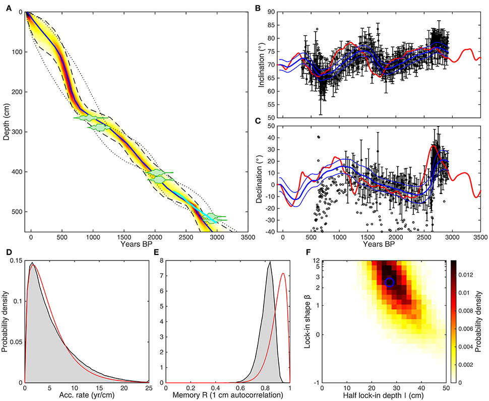
Figure 3. (A) The age-depth posterior distribution for Gyltigesjön based on paleomagnetic data (yellow/red shading) with the 95% confidence envelope (dashed black) compared to the wiggle-match chronology (cyan solid) and the 95% confidence envelope of the radiocarbon-based chronology (dotted black). Calibrated probability density curves of available macrofossil radiocarbon dates are shown for reference as green shaded areas. The blue line represents the preferred age-depth model based on the weighted mean age for each depth. (B) Inclination and (C) declination data (filled black circles) with one sigma error compared to the ARCH3k_cst.1 geomagnetic field model prediction (solid red) filtered with the preferred lock-in function (solid blue) with 1σ uncertainty envelope. Rejected data are shown as open black symbols. In the lower panels: The prior (red) and posterior (gray) distributions of (D) accumulation rate and (E) memory. (F) The posterior distribution of the half lock-in depth (l) and lock-in shape(β), where the blue circle marks the “preferred” parameters, determined by the grid cell with highest probability.

Based on the findings of Mellström et al. (2015), we use the ARCH3k_cst.1 model (Korte et al., 2009), constrained by a selection of high quality archeomagnetic data, as our input geomagnetic reference curve. The ARCH3k_cst.1 model does not have any uncertainty estimates, so we assume a constant inclination error ${\sigma }_{BI}=2^{°}$ and obtain the declination error σ_BD from (6) (see Mellström et al., 2015). The model is extrapolated to the year the cores were retrieved (2010 AD) and beyond, assuming no change in the field, which is necessary when considering that lock-in may still be on-going in the uppermost sediments. We also use the full, but less supported, age-range of the model, extending back to 2000 BC, to maximize the number of paleomagnetic measurements included in the analysis (z_lim = 550 cm).

The parameters used for the age-depth model are summarized in Table 1. For more details, see Supplementary Information and Blaauw and Christen (2011). Sediment accumulation rates in the upper part of the core investigated here are expected to vary between c. 3 and 10 years/cm (Snowball et al., 2013), so we set our prior for the accumulation rate to a gamma distribution with shape parameter 1.5, recommended by Blaauw and Christen (2011), and mean of 5 years/cm. We do not expect drastic accumulation rate changes and, therefore, set the prior for accumulation rate variability as a beta distribution with memory strength 20 and mean 0.9 (“high memory”). We divide the sequence into 25 slices, which results in (corresponding to z_lim/25). Based on the results of Mellström et al. (2015), we set l_max = 50 cm and the resolution for the discrete convolution F_res = 1 cm.

Table 1. Age-depth model parameters.

The intention with our new method is to combine all available chronological information in one age-depth model. However, for comparison purposes we present two separate age-depth models and compare them to the independent wiggle-match dated chronology. In Figure 3A we show the posterior distribution of the age-depth model based on the paleomagnetic data only. For reference we show the 95% confidence limits (dotted black lines) of an age-depth model based on all (six) available macrofossil radiocarbon determinations for the investigated depths (Snowball et al., 2013), but without using paleomagnetic data. Both age-depth models agree well within their respective uncertainties and also overlap reasonably well with the wiggle-matched chronology between 3000 and 2200 years BP (solid cyan line). Importantly, there are no apparent systematic offsets between the paleomagnetic- and radiocarbon-based chronologies.

To visualize the model-data comparison we plot paleomagnetic data and the convolved geomagnetic field model prediction (Figures 3B,C) on a “preferred” age-depth model, determined as the weighted mean age for each depth, using the “preferred” l and b (determined from the posterior density in Figure 3F) to derive λ and β for the model convolution. The comparison between the original model prediction (red lines) and the convolved model (blue lines) shows the smoothing and temporal offset (c. 200 years) induced by lock-in. If not accounted for, this would lead to systematically young ages in the paleomagnetic-based chronology (Figure 3A). Since we do not include any hard temporal constraints apart from the top of the sequence, the lock-in depth must be constrained mainly by the degree of smoothing in the paleomagnetic data compared to the geomagnetic field model prediction.

The posterior for accumulation rate is similar to the prior distribution (Figure 3D), but the posterior for the memory (Figure 3E) indicates that the data require more accumulation rate variability than suggested by the prior distribution. The posterior distribution of the lock-in parameters (Figure 3F) suggests a half lock-in depth (l) of 30.7 ± 6.5 cm (mean and standard deviation) and a lock-in shape β > 0, i.e., negative values of β are rejected.

Kälksjön Paleomagnetic Age-Depth Model

Lake Kälksjön is located in west central Sweden. The PSV record consists of paleomagnetic measurements on 940 discrete samples from six partially overlapping piston cores taken from a 7-m-long sequence (Stanton et al., 2010, 2011; Mellström et al., 2015). The upper 2 m of the record (relevant for this study) have been dated by a combination of varve counting, ¹³⁷Cs activity, Pb pollution dating, 22 bulk radiocarbon dates, 19 of which were used for the wiggle-match dating, and four macrofossil radiocarbon determinations (Mellström et al., 2015).

Similar to Gyltigesjön, we exclude declination data from the uppermost 75 cm of each core from our analyses, due to suspected core rotation. We use the same geomagnetic field input model and set z_lim = 200 cm. The prior for the accumulation rate is set to a gamma distribution with shape 1.5 and mean 20. As above, we divide the record into 25 slices, Δc = 8 cm (corresponding to z_lim/25), but due to the smaller value of we allow for more accumulation rate variability with memory strength 10 and mean 0.8. Based on the results of Mellström et al. (2015), we set l_max = 25 cm and the resolution for the discrete convolution to F_res = 0.5 cm (Table 1).

We produce a paleomagnetic-based age-depth curve (ignoring all radiocarbon dates) and one radiocarbon-based age-depth curve, using all (four) macrofossil determinations, and compare these to the independent wiggle-matched chronology (Figure 4A). As was the case for Gyltigesjön, all three chronologies are consistent within their errors and do not contain any evidence for systematic errors. We note that the paleomagnetic-based age-depth models for both Gyltigesjön and Kälksjön indicate a distinct accumulation rate change around 2600 years BP, which suggests inconsistencies between paleomagnetic data and geomagnetic field model predictions and/or unsuitable lock-in filter functions. The posterior distribution of the lock-in parameter space (Figure 4F) suggests a half lock-in depth (l) of 16.6 ± 3.3 cm (mean and standard deviation), with a weakly constrained lock-in shape, again rejecting negative β values.

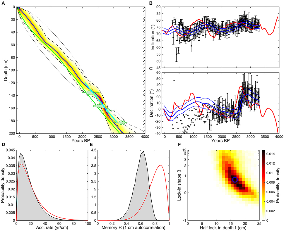
Figure 4. (A) The age-depth posterior distribution for Kälksjön based on paleomagnetic data (yellow/red shading) with the 95% confidence envelope (dashed black) compared to the wiggle-match chronology (solid cyan), the adjusted varve chronology (solid green) and the 95% confidence envelope of the radiocarbon-based chronology (dotted black). Calibrated probability density curves of available macrofossil radiocarbon dates are shown for reference as green shaded areas. The blue line represents the preferred age-depth model based on the weighted mean age for each depth. (B) Inclination and (C) declination data (filled black circles) with 1σ error compared to the ARCHk_cst.1 geomagnetic field model prediction (solid red) filtered with the preferred lock-in function (solid blue) with one sigma uncertainty envelope. Rejected data are shown as open black symbols. In the lower panels: The prior (red) and posterior (gray) distributions of (D) accumulation rate and (E) memory. (F) The posterior distribution of the half lock-in depth (l) and lock-in shape (β), where the blue circle marks the “preferred” parameters, determined by the grid cell with highest probability.

Also shown in Figure 4A (green line) is the “corrected” varve chronology from Stanton et al. (2010). Based on Pb pollution data and PSV correlations, Stanton et al. (2010) found that the original varve chronology was missing ~270 varves in the younger part of the record. The varve chronology was, therefore, corrected by evenly distributing the missing varves over the part spanning the last 1000 years. However, the wiggle-match dating by Mellström et al. (2015) suggests that an additional 213 varves may be missing further down the core. In Figure 5, we plot the Kälksjön ²⁰⁶Pb/²⁰⁷Pb data on our paleomagnetic-based chronology and compare them with three independently dated records of Pb pollution from different parts of Sweden (Brännvall et al., 1999; Bindler et al., 2009), one of which (Koltjärn) was used originally by Stanton et al. (2010). Our paleomagnetic-based chronology places the Greek-Roman Pb peak (corresponding to a decline in ²⁰⁶Pb/²⁰⁷Pb ratios around 2000 years BP) roughly 100 years too early but well within the chronological error. Otherwise the data are in good agreement, which demonstrates that the paleomagnetic-based chronology is consistent with both the wiggle-match chronology and Pb pollution data.

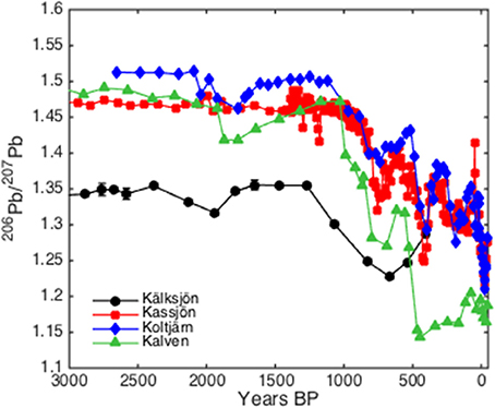
Figure 5. Kälksjön lead isotope ²⁰⁶Pb/²⁰⁷Pb ratio plotted against the age-depth curve based on paleomagnetic data (solid symbols) with linear interpolation between data points. For comparison the ²⁰⁶Pb/²⁰⁷Pb ratio for similar independently dated records from Kassjön, Koltjärn, and Kalven are also plotted.

Exploring Lock-In Parameters

To further constrain the lock-in parameters, we produced a third age-depth model for Gyltigesjön and Kälksjön, respectively, including both paleomagnetic data and all macrofossil radiocarbon determinations (see Supplementary Information). Additional temporal constraints, provided by radiocarbon determinations, do not lead to any significant changes to the paleomagnetic-based age-depth curves but provide more information on the lock-in parameters (Figures 6A,B). To compare our results to those of Mellström et al. (2015), we repeated their analysis using our new parameterized lock-in function (Figures 6C,D) with the same paleomagnetic data (binned every 7 cm and 4 cm, respectively) and Gaussian error distribution as in the original study (for a more detailed description, see Supplementary Information). Even though the two analyses were conducted over different age ranges, with variable or fixed wiggle-matched timescales and with discrete or binned data, the results still look similar. In all four cases, the posterior distribution of the lock-in parameters is centered around β = 1 (i.e., a “linear” lock-in function) with l ≈ 30 cm and l ≈ 15 cm, respectively.

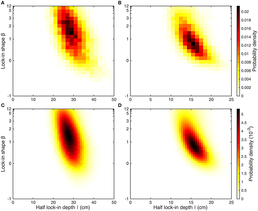
Figure 6. The posterior distribution of lock-in parameters for (A) Gyltigesjön and (B) Kälksjön derived from age-depth models based on both paleomagnetic and radiocarbon data, compared to (C,D) reanalyzed results of Mellström et al. (2015), based on binned paleomagnetic data and wiggle-match dated timescales.

Recovering High-Frequency Field Variations

To demonstrate how the lock-in parameters, identified with our method, can be used to recover high-frequency field variations we use them to deconvolve the entire Gyltigesjön PSV record. Deconvolution is sensitive to noise, so to attempt to isolate a robust signal we fit the inclination and declination data with cubic smoothing splines weighted by data uncertainties. The spline fits were then transformed to Cartesian coordinates (assuming a unit sphere) and deconvolved by division in the frequency domain using the lock-in filter with highest probability from Figure 6C (β = 1.3, l = 28). The results are shown in Figure 7 on the original published age-depth model, including the wiggle-matched dating (Snowball et al., 2013) and compared to ARCH3k_cst.1 and pfm9k.1b (Nilsson et al., 2014) model predictions. The recent part of the deconvolved record (<3500 years) is essentially constrained to fit ARCH3k_cst.1, although with a few clear differences such as the enhanced eastward declination swing around 2650 years BP (known as feature “f”; Turner and Thompson, 1981) and the shallower inclination around 2250 years BP. The older and independent part of the “restored” PSV record, which is the main gain of this approach, indicates that it is possible to extract a similar range of field variability in sedimentary data as in archeomagnetic data.

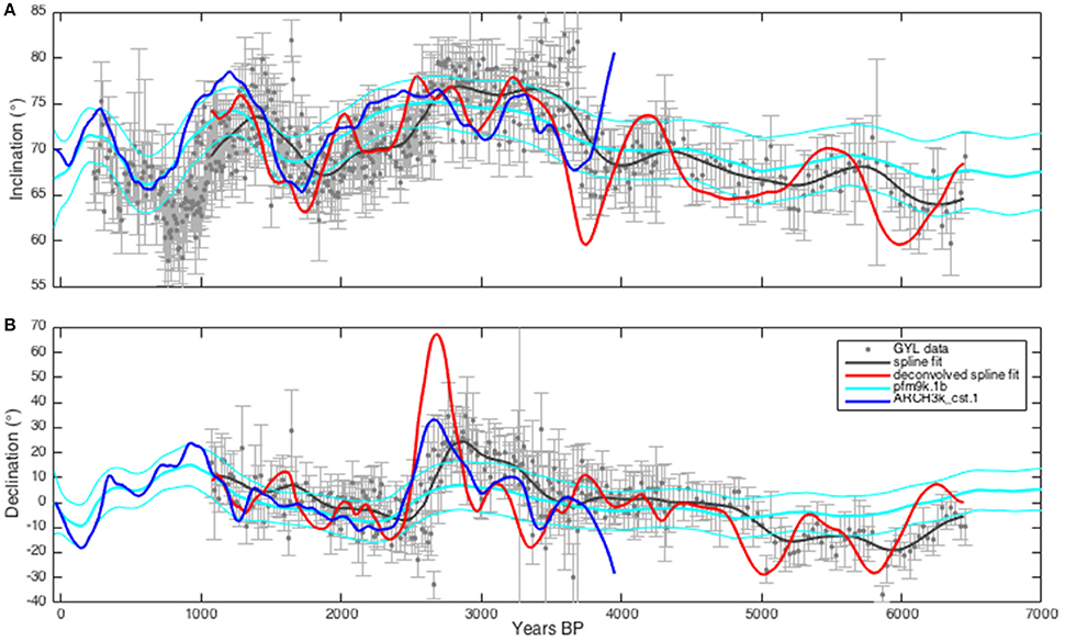
Figure 7. (A) Inclination and (B) declination data (filled gray circles) with 1σ error from Lake Gyltigesjön. A smoothing spline fitted to the data (solid dark gray) deconvolved using the half lock-in depth (l ≈ 28) and lock-in shape (β ≈ 1.3) with highest probability from Figure 6C (solid red). The pfm9k.1b (solid cyan) and ARCHk_cst.1 (solid blue) geomagnetic field model predictions with 1σ uncertainty envelope (pfm9k.1b) are shown for comparison.

Discussion

The Lock-In Function

The method presented here enables the study of variations in the lock-in process in many lake or marine settings where expensive wiggle-match dating or other high-precision dating methods are either not available or applicable. Our analyses reproduce the results of Mellström et al. (2015), which supports the conclusion that the “linear” lock-in function is the most appropriate of available lock-in functions for the Gyltigesjön and Kälksjön records. In general, however, we conclude that the method does not distinguish much between variations in lock-in shape, but is mainly sensitive to the half lock-in depth, which is deeper in Gyltigesjön than in Kälksjön. The physical cause of pDRM in these sediments remains unclear but may be related to the unusually high organic content, in particular for Gyltigesjön (Mellström et al., 2015).

The parameterized lock-in function presented in this paper is able to reproduce most lock-in functions proposed in the literature. Although we have made no attempt to explain the underlying physical process, we propose that using this or other similar functions is better than ignoring lock-in altogether when considering paleomagnetic data for geomagnetic field modeling or for dating. Our new method provides a platform that could be used to experiment with other, more physically motivated (e.g., Egli and Zhao, 2015), variations of filter functions, as long as they can be defined with a limited number of parameters.

Age-Depth Model Applications

Although the method presented in this paper is primarily intended to be used to explore pDRM effects in sediments, it can also be used as a complement to conventional radiocarbon dating for sedimentary archives, particularly in areas where suitable materials for dating are scarce. The uncertainty of age-depth models based on paleomagnetic data will, however, only be as good as the regional geomagnetic field reference curve. When considering lock-in effects, the quality of the geomagnetic field model predictions depends on the availability of archeomagnetic data, which effectively restricts the method to sites in the northern hemisphere and the past 3–4 millennia. However, we note that the method could potentially also be used with a wider range of geomagnetic field models based on both archeomagnetic and sedimentary data, such as pfm9k.1b, with the caveat that temporal offsets caused by lock-in processes may not be appropriately adjusted for. This would increase the potential application of the dating method in time, beyond the archeomagnetic models, and to the southern hemisphere.

Implications for Geomagnetic Field Reconstructions

As noted above, both paleomagnetic age-depth models for Gyltigesjön (Figure 3) and Kälksjön (Figure 4) contain a change in accumulation rate around 2600 years BP, which is not supported by the wiggle-match timescales (Mellström et al., 2015). It appears that the age-depth models require high accumulation rates prior to 2600 years to minimize lock-in smoothing of the geomagnetic field model prediction over this time interval and to better capture the large amplitude eastward declination swing (feature “f”) predicted by the data. This implies that the geomagnetic field model prediction might be too smooth at around this time, i.e., that the declination swing was more pronounced than the model predicts, which is supported by comparison to the deconvolved Gyltigesjön record (Figure 7). Likewise, the shallow inclination predicted by the deconvolved record at around 2250 years BP could also be a real feature of the field that is not captured by the archeomagnetic model.

These observations highlight the potential limitations of archeomagnetic field models, which lack data from high latitude locations such as the lake sites, and why it is important to include sedimentary data in global geomagnetic field models. By including assumptions about lock-in processes we have shown that it is possible to recover high-frequency variations from sedimentary paleomagnetic data and remove potential systematic age uncertainties (Nilsson et al., 2014). In Figure 7, we demonstrate this by deconvolving the Gyltigesjön record. However, with such an approach it will always be difficult to isolate the real signal and avoid amplifying noise. We propose that a better method would be to incorporate the full age-depth method presented here into the modeling, and to fit the sedimentary data with a lock-in filtered model prediction (Nilsson and Suttie, 2016). With a correct understanding of the smoothing effect of the lock-in process, e.g., using updated lock-in filter functions, it should be possible to recover the higher frequency geomagnetic field components that are currently captured by archeomagnetic data throughout the Holocene.

Conclusions

We have presented a novel Bayesian method to simultaneously model lock-in processes and construct an age-depth model based on paleomagnetic data and archeomagnetic field model predictions. The method provides, for the first time, a way to constrain the effects of pDRM acquisition in sediments in the absence of high-precision dating methods. This is the first paleomagnetic method that addresses problems related to lock-in delay in age-depth modeling and has potential to be used to complement conventional radiocarbon dating for sedimentary archives. Finally, we have demonstrated how the identified lock-in parameters can be used to recover high-frequency geomagnetic field variations from sedimentary paleomagnetic data by deconvolving the Gyltigesjön Lake PSV record which can lead to an increase in the fidelity of geomagnetic field models.

The deconvolved Gyltigesjön PSV data shown in Figure 7 are provided in the EarthRef.org Digital Archive (ERDA, http://www.earthref.org) by searching for Gyltigesjön or the title of this study.

Author Contributions

AN wrote main manuscript with contributions from both NS and MH. AN and NS did most of the work on developing the methodology.

Conflict of Interest Statement

The authors declare that the research was conducted in the absence of any commercial or financial relationships that could be construed as a potential conflict of interest.

Acknowledgments

This work was funded by the Swedish Research Council (2014-4125), the Crafoord Foundation (20150843), and the Natural Environment Research Council, UK (NE/I013873/1). We thank Andrés Christen and Maarten Blaauw for providing helpful advice regarding the Bacon implementation. Andrew P. Roberts and Shuhui Cai are thanked for their thorough reviews, which substantially improved the manuscript.

Supplementary Material

The Supplementary Material for this article can be found online at: https://www.frontiersin.org/articles/10.3389/feart.2018.00039/full#supplementary-material

References

Anson, G. L., and Kodama, K. P. (1987). Compaction-induced inclination shallowing of the post-depositional remanent magnetization in a synthetic sediment. Geophys. J. R. Astron. Soc. 88, 673–692. doi: 10.1111/j.1365-246X.1987.tb01651.x
Bindler, R., Renberg, I., Rydberg, J., and Andrén, T. (2009). Widespread waterborne pollution in central Swedish lakes and the Baltic Sea from pre-industrial mining and metallurgy. Environ. Pollut. 157, 2132–2141. doi: 10.1016/j.envpol.2009.02.003
Blaauw, M., and Christen, J. A. (2011). Flexible paleoclimate age-depth models using an autoregressive gamma process. Bayesian Anal. 6, 457–474. doi: 10.1214/11-BA618
Bleil, U., and Dobeneck, T. (1999). “Geomagnetic events and relative paleointensity records – clues to high-resolution paleomagnetic chronostratigraphies of Late Quaternary marine sediments?” in Use of Proxies in Paleoceanography, eds G. Fischer and G. Wefer (Berlin; Heidelberg: Springer), 635–654.
Blow, R. A., and Hamilton, N. (1978). Effect of compaction on the acquisition of a detrital remanent magnetization in fine-grained sediments. Geophys. J. R. Astron. Soc. 52, 13–23. doi: 10.1111/j.1365-246X.1978.tb04219.x
Bowles, J. (2007). Coring-related deformation of Leg 208 sediments from Walvis Ridge: implications for paleomagnetic data. Phys. Earth Planet. Inter. 161, 161–169. doi: 10.1016/j.pepi.2007.01.010
Brännvall, M.-L., Bindler, R., Renberg, I., Emteryd, O., Bartnicki, J., and Billström, K. (1999). The medieval metal industry was the cradle of modern large-scale atmospheric lead pollution in northern Europe. Environ. Sci. Technol. 33, 4391–4395. doi: 10.1021/es990279n
Bronk Ramsey, C. (2009). Bayesian analysis of radiocarbon dates. Radiocarbon 51, 337–360. doi: 10.1017/S0033822200033865
Brown, M., Donadini, F., Nilsson, A., Panovska, S., Frank, U., Korhonen, K., et al. (2015). GEOMAGIA50.v3: 2. A new paleomagnetic database for lake and marine sediments. Earth Planets Space 67, 1–19. doi: 10.1186/s40623-015-0233-z
Channell, J. E. T., and Guyodo, Y. (2004). “The Matuyama Chronozone at ODP Site 982 (Rockall Bank): evidence for decimeter-scale magnetization lock-in depths,” in Timescales of the Paleomagnetic Field, Geophysical Monograph Series, Vol. 145, eds J. E. T. Channell, D. V. Kent, W. Lowrie, and J. G. Meert (Washington, DC: AGU), 205–219.
Christen, J. A., and Fox, C. (2010). A general purpose sampling algorithm for continuous distributions (the t-walk). Bayesian Anal. 5, 263–281. doi: 10.1214/10-BA603
Denham, C. R., and Chave, A. D. (1982). Detrital remanent magnetization: viscosity theory of the lock-in zone. J. Geophys. Res. 87, 7126–7130. doi: 10.1029/JB087iB08p07126
Egli, R., and Zhao, X. (2015). Natural remanent magnetization acquisition in bioturbated sediment: general theory and implications for relative paleointensity reconstructions. Geochem. Geophys. Geosyst. 16, 995–1016. doi: 10.1002/2014GC005672
Fisher, R. (1953). Dispersion on a sphere. Proc. R. Soc. London Ser. A 217, 295–305. doi: 10.1098/rspa.1953.0064
Gravenor, C. P., Symons, D. T. A., and Coyle, D. A. (1984). Errors in the anisotropy of magnetic susceptibility and magnetic remanence of unconsolidated sediments produced by sampling methods. Geophys. Res. Lett. 11, 836–839. doi: 10.1029/GL011i009p00836
Hamano, Y. (1980). An experiment on the post-depositional remanent magnetization in artificial and natural sediments. Earth Planet. Sci. Lett. 51, 221–232. doi: 10.1016/0012-821X(80)90270-8
Heslop, D., Roberts, A. P., Chang, L., Davies, M., Abrajevitch, A., and De Deckker, P. (2013). Quantifying magnetite magnetofossil contributions to sedimentary magnetizations. Earth Planet. Sci. Lett. 382, 58–65. doi: 10.1016/j.epsl.2013.09.011
Hyodo, M. (1984). Possibility of reconstruction of the past geomagnetic field from homogeneous sediments. J. Geomagn. Geoelectr. 36, 45–62. doi: 10.5636/jgg.36.45
Irving, E., and Major, A. (1964). Post-depositional detrital remanent magnetization in a synthetic sediment. Sedimentology 3, 135–143. doi: 10.1111/j.1365-3091.1964.tb00638.x
Katari, K., Tauxe, L., and King, J. (2000). A reassessment of post-depositional remanent magnetism: preliminary experiments with natural sediments. Earth Planet. Sci. Lett. 183, 147–160. doi: 10.1016/S0012-821X(00)00255-7
Kent, D. V. (1973). Post-depositional remanent magnetisation in deep-sea sediment. Nature 246, 32–34. doi: 10.1038/246032a0
Kent, D. V., and Schneider, D. A. (1995). Correlation of paleointensity variation records in the Brunhes/Matuyama polarity transition interval. Earth Planet. Sci. Lett. 129, 135–144. doi: 10.1016/0012-821X(94)00236-R
Khokhlov, A., and Hulot, G. (2016). Principal component analysis of palaeomagnetic directions: converting a maximum angular deviation (MAD) into an α95 angle. Geophys. J. Int. 204, 274–291. doi: 10.1093/gji/ggv451
Kirschvink, J. L. (1980). The least-squares line and plane and the analysis of palaeomagnetic data. Geophys. J. R. Astron. Soc. 62, 699–718. doi: 10.1111/j.1365-246X.1980.tb02601.x
Korte, M., Constable, C., Donadini, F., and Holme, R. (2011). Reconstructing the holocene geomagnetic field. Earth Planet. Sci. Lett. 312, 497–505. doi: 10.1016/j.epsl.2011.10.031
Korte, M., Donadini, F., and Constable, C. G. (2009). Geomagnetic field for 0-3 ka: 2. A new series of time-varying global models. Geochem. Geophys. Geosyst. 10:Q06008. doi: 10.1029/2008GC002297
Larrasoaña, J. C., Liu, Q., Hu, P., Roberts, A. P., Mata, P., Civis, J., et al. (2014). Paleomagnetic and paleoenvironmental implications of magnetofossil occurrences in late Miocene marine sediments from the Guadalquivir Basin, SW Spain. Front. Microbiol. 5:71. doi: 10.3389/fmicb.2014.00071
Licht, A., Hulot, G., Gallet, Y., and Thébault, E. (2013). Ensembles of low degree archeomagnetic field models for the past three millennia. Phys. Earth Planet. Inter. 224, 38–67. doi: 10.1016/j.pepi.2013.08.007
Løvlie, R. (1976). The intensity pattern of post-depositional remanence acquired in some marine sediments deposited during a reversal of the external magnetic field. Earth Planet. Sci. Lett. 30, 209–214. doi: 10.1016/0012-821X(76)90247-8
Lund, S. P., and Keigwin, L. (1994). Measurement of the degree of smoothing in sediment paleomagnetic secular variation records: an example from late Quaternary deep-sea sediments of the Bermuda Rise, western North Atlantic Ocean. Earth Planet. Sci. Lett. 122, 317–330. doi: 10.1016/0012-821X(94)90005-1
Mao, X., Egli, R., Petersen, N., Hanzlik, M., and Zhao, X. (2014). Magnetotaxis and acquisition of detrital remanent magnetization by magnetotactic bacteria in natural sediment: first experimental results and theory. Geochem. Geophys. Geosyst. 15, 255–283, doi: 10.1002/2013GC005034
Mellström, A., Muscheler, R., Snowball, I., Ning, W., and Haltia, E. (2013). Radiocarbon wiggle-match dating of bulk sediments—How accurate can it be? Radiocarbon 55, 1173–1186. doi: 10.1017/S0033822200048086
Mellström, A., Nilsson, A., Stanton, T., Muscheler, R., Snowball, I., and Suttie, N. (2015). Post-depositional remanent magnetization lock-in depth in precisely dated varved sediments assessed by archaeomagnetic field models. Earth Planet. Sci. Lett. 410, 186–196. doi: 10.1016/j.epsl.2014.11.016
Meynadier, L., and Valet, J.-P. (1996). Post-depositional realignment of magnetic grains and asymmetrical saw-tooth patterns of magnetization intensity. Earth Planet. Sci. Lett. 140, 123–132. doi: 10.1016/0012-821X(96)00018-0
Nilsson, A., Holme, R., Korte, M., Suttie, N., and Hill, M. J. (2014). Reconstructing Holocene geomagnetic field variation: new methods, models and implications. Geophys. J. Int. 198, 229–248, doi: 10.1093/gji/ggu120
Nilsson, A., and Suttie, N. (2016). Palaeomagnetic dating method accounting for post-depositional remanence and its application to geomagnetic field modelling. American Geophysical Union Fall General Assembly 2016, Abstract #GP14C-05.
Otofuji, Y., and Sasajima, S. (1981). A magnetization process of sediments: laboratory experiments on post-depositional remanent magnetization. Geophys. J. R. Astron. Soc. 66, 241–259. doi: 10.1111/j.1365-246X.1981.tb05955.x
Pavón-Carrasco, F. J., Osete, M. L., Torta, J. M., and De Santis, A. (2014). A geomagnetic field model for the Holocene based on archaeomagnetic and lava flow data. Earth Planet. Sci. Lett. 388, 98–109. doi: 10.1016/j.epsl.2013.11.046
Roberts, A. P., Florindo, F., Chang, L., Heslop, D., Jovane, L., and Larrasoaña, J. C. (2013b). Magnetic properties of pelagic marine carbonates. Earth Sci. Rev. 127, 111–139. doi: 10.1016/j.earscirev.2013.09.009
Roberts, A. P., Tauxe, L., and Heslop, D. (2013a). Magnetic paleointensity stratigraphy and high-resolution Quaternary geochronology: successes and future challenges. Quat. Sci. Rev. 61, 1–16. doi: 10.1016/j.quascirev.2012.10.036
Roberts, A. P., and Winklhofer, M. (2004). Why are geomagnetic excursions not always recorded in sediments? Constraints from post-depositional remanent magnetization lock-in modelling. Earth Planet. Sci. Lett. 227, 345–359. doi: 10.1016/j.epsl.2004.07.040
Sagnotti, L., Budillon, F., Dinarès-Turell, J., Iorio, M., and Macrì, P. (2005). Evidence for a variable paleomagnetic lock-in depth in the Holocene sequence from the Salerno Gulf (Italy): implications for “high-resolution” paleomagnetic dating. Geochem. Geophys. Geosyst. 6, Q11013. doi: 10.1029/2005GC001043
Simon, Q., Bourlès, D. L., Thouveny, N., Horng, C.-S., Valet, J.-P., Bassinot, F., et al. (2018). Cosmogenic signature of geomagnetic reversals and excursions from the Réunion event to the Matuyama–Brunhes transition (0.7–2.14 Ma interval). Earth Planet. Sci. Lett. 482, 510–524. doi: 10.1016/j.epsl.2017.11.021
Snowball, I., Mellström, A., Ahlstrand, E., Haltia, E., Nilsson, A., Ning, W., et al. (2013). An estimate of post-depositional remanent magnetization lock-in depth in organic rich varved lake sediments. Global Planet. Change 110, 264–277. doi: 10.1016/j.gloplacha.2013.10.005
Snowball, I., and Thompson, R. (1990). A stable chemical remanence in Holocene sediments. J. Geophys. Res. 95, 4471–4479. doi: 10.1029/JB095iB04p04471
Stanton, T., Nilsson, A., Snowball, I., and Muscheler, R. (2011). Assessing the reliability of Holocene relative palaeointensity estimates: a case study from Swedish varved lake sediments. Geophys. J. Int. 187, 1195–1214. doi: 10.1111/j.1365-246X.2011.05049.x
Stanton, T., Snowball, I., Zillén, L., and Wastegård, S. (2010). Validating a Swedish varve chronology using radiocarbon, palaeomagnetic secular variation, lead pollution history and statistical correlation. Quat. Geochron. 5, 611–624. doi: 10.1016/j.quageo.2010.03.004
Striberger, J., Björck, S., Ingólfsson, Ó., Kjær, K. H., Snowball, I., and Uvo, C. B. (2011). Climate variability and glacial processes in eastern Iceland during the past 700 years based on varved lake sediments. Boreas 40, 28–45. doi: 10.1111/j.1502-3885.2010.00153.x
Suganuma, Y., Okuno, J., Heslop, D., Roberts, A. P., Yamazaki, T., and Yokoyama, Y. (2011). Post-depositional remanent magnetization lock-in for marine sediments deduced from 10Be and paleomagnetic records through the Matuyama-Brunhes boundary. Earth Planet. Sci. Lett. 311, 39–52. doi: 10.1016/j.epsl.2011.08.038
Tarduno, J. A., Tian, W., and Wilkison, S. (1998). Biogeochemical remanent magnetization in pelagic sediments of the western equatorial Pacific Ocean. Geophys. Res. Lett. 25, 3987–3990. doi: 10.1029/1998GL900079
Keywords: paleomagnetism, geomagnetic field, post-depositonal remanent magnetization, lock-in, age-depth models
Citation: Nilsson A, Suttie N and Hill MJ (2018) Short-Term Magnetic Field Variations From the Post-depositional Remanence of Lake Sediments. Front. Earth Sci. 6:39. doi: 10.3389/feart.2018.00039
Received: 21 December 2017; Accepted: 03 April 2018;
Published: 19 April 2018.
Edited by:
Christopher Davies, University of Leeds, United KingdomReviewed by:
Andrew Philip Roberts, Australian National University, AustraliaShuhui Cai, Scripps Institution of Oceanography, University of California, San Diego, United States
Copyright © 2018 Nilsson, Suttie and Hill. This is an open-access article distributed under the terms of the Creative Commons Attribution License (CC BY). The use, distribution or reproduction in other forums is permitted, provided the original author(s) and the copyright owner are credited and that the original publication in this journal is cited, in accordance with accepted academic practice. No use, distribution or reproduction is permitted which does not comply with these terms.
*Correspondence: Andreas Nilsson, andreas.nilsson@geol.lu.se