Sub-seasonal Predictability of the Onset and Demise of the Rainy Season over Monsoonal Regions

Introduction

The deterministic prediction of the evolution of monsoon systems has proven to be a challenging task (Charney and Shukla, 1982; Webster et al., 1998; Krishnamurthy and Shukla, 2012). The most successful deterministic predictions of monsoon systems to date consist of predicting the large-scale component of the flow, defined as the primary modes of variability (Zhou and Zou, 2010; Zuo et al., 2013; Wang et al., 2015). However, regional features of monsoon precipitation anomalies remain highly unpredictable (Zhou and Zou, 2010).

Although it is challenging to predict the full evolution of monsoon systems, there is evidence that it is possible to predict the onset dates of monsoon systems on sub-seasonal to seasonal timescales using large-scale monsoon indexes (Vellinga et al., 2013; Alessandri et al., 2015). Alessandri et al. (2015) showed that the onset of the Indian summer monsoon (ISM) can be predicted on sub-seasonal timescales using retrospective forecasts with the prediction system developed at Centro Euro-Mediterraneo sui Cambiamenti Climatici (CMCC). They used two different indices based on large-scale features of the ISM and found that the onset date can be predicted skillfully as much as a month in advance. Vellinga et al. (2013) investigated the forecast skill for the onset date of the monsoon in the Sahel region of West Africa and verified probabilistic skill at 2–3 months lead-time using the operational seasonal forecasting system of the UK Met Office (GloSea4).

In contrast, attempts to represent the onset and demise of monsoons using regional features, such as simulated gridded wind and precipitation, have proved to be more challenging (Cherchi and Navarra, 2003; Li and Zhang, 2009). Both Cherchi and Navarra (2003) and Li and Zhang (2009) evaluated the representation of the onset and demise of the Asian summer monsoon in global circulation models using Atmospheric Model Intercomparison Project (AMIP) style simulations. These studies found that the models performed better at representing the onset and demise of the Asian summer monsoon when the onset and demise were defined in terms of monsoon circulation (e.g., gridded 850 hPa kinetic energy or wind), rather than in terms of gridded precipitation.

In this work we take a different approach from previous studies. Instead of predicting the onset (or demise) dates of the monsoon system itself, which is a complex large-scale phenomenon, we will predict the onset and the demise dates of the rainy season associated with a particular monsoon system. Although monsoon indices can provide useful information about the large-scale properties of monsoon systems, the utility of this knowledge is somewhat limited at the local level. Our method, however, allows us to determine the characteristics of the rainy season over every grid point, providing the user with information at the same spatial resolution as the dataset used. In addition, instead of relying completely on the model's ability to represent the onset and demise of the rainy season we use a hybrid methodology that combines observations and simulations by appending the model's predictions to observations prior to the initialization date of the forecasts. Using this methodology, we demonstrate that it is possible to make skillful sub-seasonal forecasts of the onset and demise dates of the rainy season for certain monsoon systems. Based on this forecast skill, our methodology provides a complimentary forecast to the prediction of large-scale monsoon indices that can be used at the local level.

Accurate prediction of these dates are not only relevant to predicting the onset of the monsoon system as a whole but can also provide valuable information for decision makers. Sectors related to water management such as agriculture, management of waterborne diseases, and electric energy generation would greatly benefit from the prediction of the dates of onset or demise of monsoons. The objective of this work is to evaluate how far in advance model re-forecasts perform better than using climatological values to forecast the onset and demise of the rainy season over some of the monsoonal regions. We will show that models produce skillful predictions of the onset and demise dates of the rainy season on sub-seasonal timescales for several of these regions. Section “Data and Methods” presents the data and methods used in this study. The forecast of the onset of the rainy season is explored in Section “The Onset of the Rainy Season”. Section “The Demise of the Rainy Season” explores the forecast of the demise of the rainy season. Section “Precipitation Bias and Time Series Discontinuity” investigates the role of simulated precipitation bias in the predictability of the onset and demise dates of the rainy season. A discussion and the conclusions are presented in Section “Precipitation Bias and Time Series Discontinuity”.

Data and Methods

Onset and Demise Dates of the Rainy Season in Observations

The onset and demise dates of the rainy and dry seasons are characterized here based on a method designed to capture a seasonal change in the precipitation regime and adapted to be used with model forecasts or hindcasts. This method uses only precipitation data and was developed by Bombardi and Carvalho (2009), based on the method proposed by Liebmann and Marengo (2001). In this work we use daily precipitation from the Climate Prediction Center Unified Precipitation (CPC_UNI) from 1979 to 2014 (Xie et al., 2007; Chen et al., 2008) and daily precipitation estimates from the Tropical Rainfall Measuring Mission (TRMM; Huffman et al., 2007) from 1998 to 2013 (see Appendix).

As the procedure for determining onset and demise has undergone several improvements since it was originally proposed we present a full description of the methodology here (illustrated in Figure 1). The onset or demise date for each grid point is calculated from Equation 1:

where S(n) is the accumulated precipitation deviation from the annual mean at day “n,” P(i) is the daily precipitation at day “i,” “P_C” is the annual daily average precipitation (annual climatological precipitation rate), and “t₀” is the starting date for the calculations. The calculation starts on t₀ up to a full year (N = t₀ + 364). Therefore, n ranges from t₀ to N. The calculation of the onset of the rainy season always starts from the same day of the year for every year.

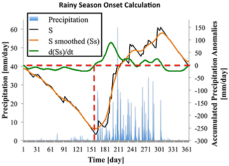
Figure 1. Example of the calculation of the onset of the rainy season for a single year for a grid point over central India. The left axis shows observed precipitation values and the right axis shows the values of S, S smoothed (Ss), and the first derivative of Ss. The horizontal dashed line shows the zero line for accumulated anomalies and the vertical dashed line shows the date of the onset of the rainy season.

The choice of t₀ depends on the region of interest. For example, if the region of interest is the Indian subcontinent, one could use a date in early April as t₀. Since according to the Indian Meteorological Department the onset of the rainy season does not start before May 10th, a date in early April would be well within the dry season. However, if the region of interest is a large domain such as the entire continent of South America or Africa, t₀ has to vary from grid point to grid point. The reason for that is that the onset and demise dates over all of South America and Africa will vary substantially from place to place.

In previous studies (Bombardi and Carvalho, 2009; Bombardi et al., 2015, 2016) we used the minimum and maximum dates of the climatological annual cycle of precipitation as t₀ dates from which to determine the onset and demise dates, respectively. Although this procedure works well for South America, it generates too many false onsets for India. This problem occurs because the minimum of the annual cycle sometimes falls immediately after the end of the rainy season in the Indian monsoon regions. Therefore, a better way to define t₀ is to find the dates of minimum and maximum of the first harmonic of the climatological annual cycle of precipitation with t₀ for the onset (demise) corresponding to the minimum (maximum).

If we start the calculation during the dry season, S (black line in Figure 1) will initially assume negative values. Once the rainy season starts, there will be an inflection in S. In order to avoid false onsets or demises, the S curve is smoothed (orange line in Figure 1, Ss) using a 3-point moving average and we take the first derivative of the smoothed S [green line in Figure 1, d(Ss)/dt] curve. Finally, starting from t₀, the first day when the derivative crosses from negative to positive values is considered the onset of the rainy season, as long as the positive values persist for 3 days. Rainy season demise is calculated in a similar manner, but now t₀ is selected during the wet season. The first day when the derivative crosses from positive to negative values (and the negative values persists for 3 days) is considered the demise of the rainy season. To further ensure that there are no false onset or demise dates, after the onset and demise dates are calculated we exclude outliers. We define outliers as values that are 3 times the interquartile range above or below the median of the time series of onset or demise dates.

Since we always calculate S using a full year of data, the last year in the dataset might create a boundary condition issue. To solve this problem we apply a boundary constraint to the smoothing of the time series that approximates the “minimum roughness” boundary constraint (see Mann, 2004). This constraint is applied by simply mirroring the precipitation data at the end of the time series in both “x” and “y” axes. That is, we simply add extra data points to the end of the time series. This extension of the time series is only used to assure that the smoothing of the S curve is correct at the boundaries.

The method does not require all days of the year; it simply requires a reasonable choice for the starting date t₀ and the climatological value for the annual daily average precipitation P_C. The method does require, however, a dataset that covers the period between t₀ and the onset (or demise) of the rainy season. We choose to use a full year in our calculations simply to guarantee that the onset or demise dates can be defined for every grid point, since the rainy season varies substantially from region to region. This is done to guarantee that the methodology is applied consistently at every grid point.

Onset and Demise Dates of the Rainy Season in Hindcasts

We use simulations from three global coupled models participating in the Sub-seasonal-to-Seasonal (S2S) project (Robertson et al., 2015): the China Meteorological Administration (CMA) model (Wu et al., 2010, 2014); the Japan Meteorological Agency (JMA) model (http://www.jma.go.jp/jma/jma-eng/jma-center/nwp/outline2013-nwp/index.htm); and the NCEP model (Saha et al., 2010, 2014). Table 1 summarizes the model information and details of the hindcasts. These models are examples of models that are producing S2S data and are selected only on the basis of data availability.

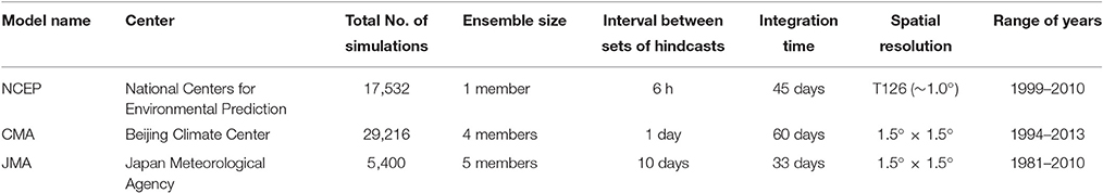
Table 1. Models' information summary.

To evaluate the skill of sub-seasonal hindcasts in forecasting the onset and demise dates of the rainy season we had to modify our methodology due to the short lead-time of the hindcasts (e.g., 45 days). The first day of each hindcast was discarded and the prediction was appended to observational data that occurred prior to the forecast initialization so that it would amount to a full year of data. In this work, the CPC_UNI and TRMM (see Appendix) precipitation data were interpolated to the grid of each S2S model prior to any calculation. We used the observed climatological values for P_C and t₀. In addition, we also applied the approximation to the “minimum roughness” boundary constraint, as noted above.

We calculate the onset and demise dates using all the hindcasts available. This is done by defining one onset date and one demise date for each grid point for every member of the S2S dataset. Once all of the onset and demise dates are identified we select only the hindcasts in which the onset or demise of the rainy season was found within the simulated period for evaluation of forecast skill. We also only analyze the results over regions where the explained variance of the first harmonic of the climatological annual cycle is above 30%, thus excluding regions that do not experience well-defined rainy and dry seasons.

The Onset of the Rainy Season

Onset Date Climatology

Figure 2 shows the median and the interquartile range of rainy season onset dates over the tropics and subtropics. The figure also indicates the domains selected to study specific monsoonal regions (black boxes), namely the North American monsoon (e.g., Adams and Comrie, 1997; Vera et al., 2006), the South American monsoon (e.g., Vera et al., 2006; Marengo et al., 2012; Carvalho and Cavalcanti, 2016), the West Africa monsoon (e.g., Nicholson, 2013), the East African monsoon (e.g., Nairobi, 1979; Mutai and Ward, 2000), the Indian monsoon (e.g., Webster et al., 1998; Krishnamurthy and Shukla, 2000; Prasad, 2005), the East Asia monsoon (e.g., Wang et al., 2001; Yihui and Chan, 2005), and the Northern Australia monsoon (e.g., Hendon and Liebmann, 1990).

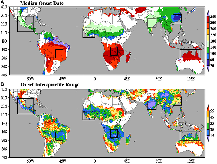
Figure 2. (A) Median onset date [DOY or Julian day] and (B) interquartile range of onset dates calculated from CPC_UNI data (1979–2014). The boxes indicate monsoonal regions of interest. We mask regions where explained variance of the first harmonic of the mean annual cycle of observed precipitation is small (<30%).

The latitudinal variation of rainy season onset dates clearly follows the seasonal evolution of convection, with the onset of the rainy season usually occurring during spring in each hemisphere (Figure 2A). Some monsoonal regions show relatively large variability in the dates of onset of the rainy season (e.g., the eastern flank of the North American, South American, West Africa, East Asian, and Northern Australia monsoon regions), while others are more consistent (e.g., the western flank of the North American, East African, and the Indian monsoon regions; Figure 2B).

Onset Date Hindcasts

Figure 3 shows the lead-time Root-Mean-Square-Error (RMSE) of onset dates for the three models considered and the multi-model ensemble (MME). The MME was generated by averaging the simulated daily precipitation of all members, which were initialized on the same day, for all three models. For the days where the JMA model was not initialized the MME consists of the average between NCEP and CMA simulations only. Lead-time zero indicates the observed onset of the rainy season. We use the observed climatology as the benchmark for comparison. That is, the goal of Figure 3 is to show whether or not (and how far in advance) the models outperform the observed climatology in predicting the onset of the rainy season.

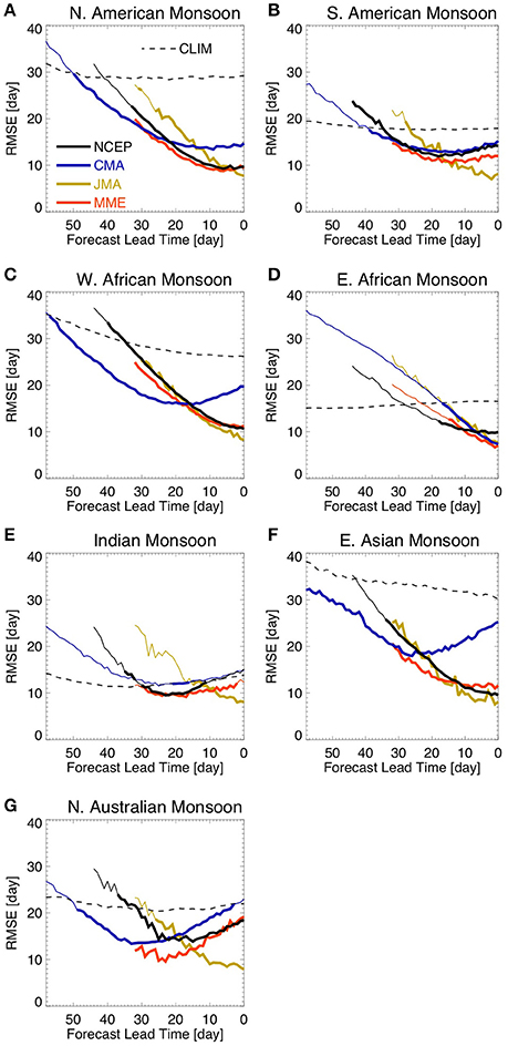
Figure 3. Lead-time RMSE of rainy season onset date forecasts. The figure shows results for (A) North American Monsoon, (B) South American Monsoon, (C) West African Monsoon, (D) East African Monsoon, (E) Indian Monsoon, (F) East Asian Monsoon, and (G) Northern Australian Monsoon. Lead-time 0 (zero) refers to the observed onset date. Thick lines show lead times where the RMSE of hindcasts is smaller than the RMSE related to the climatology and their difference is statistically significant at 5% level according to an f-test of the squared errors. The dashed line shows the RMSE in relation to the climatology for the CMA model grid for the sole purpose of visualization.

The dashed line (Figure 3) represents the average error one would observe if climatology were used to predict the onset of the rainy season. Since we interpolated the observations to the model's grids, the error in relation to the climatology differs from model to model due to the differences in spatial resolution (not shown). In addition, due to the fact that the onset of the rainy season happens at a different time of the year from grid point to grid point, the error in relation to the climatology also varies with lead-time, as we only consider grid points where the onset of the rainy season was identified in the hindcasts. The monsoonal regions of interest are relatively large and the simulation time is relative short. Therefore, the onset or demise of the rainy season at a given time might be defined for only a fraction of grid points in each region. As an example, the onset date RMSE in relation to the climatology calculated for the CMA grid is shown in Figure 3, however, the skill of each model is evaluated against the climatological values based on its own grid. To reduce the number of degrees of freedom, the errors are spatially averaged over the region of interest for each hindcast. That is, first the errors are calculated for every grid point within the region of interest and then they are spatially averaged for each ensemble member.

We find that all three models outperform the climatology in predicting the rainy season onset date over the North American (Figure 3A), the South American (Figure 3B), the West African (Figure 3C), and the East Asian (Figure 3F) monsoon regions by as much as 25–30 days in advance. The models also show good skill for the North Australian monsoon region, although the CMA model shows an inflection in the forecast error with errors growing after 30-day lead-time until the onset date (Figure 3G). Over the East African (Figure 3D) and the Indian (Figure 3E) monsoon regions, however, the models do not perform as well in comparison to the climatology at sub-seasonal timescales. As expected, the MME often has the best skill (Figure 3).

To evaluate the probabilistic forecast skill of the onset date we calculated the Heidke Skill Score (HSS) using a three by three contingency table. The observational values were divided into three equally likely categories (i.e., terciles). The tercile values are determined from the spatially averaged observed time series and the same tercile values were used for each hindcast lead-time. The HSS is the proportion of correct forecasts that would be achieved by random forecasts that are statistically independent of the observations (Wilks, 2006). A negative value indicates that a forecast is correct by chance. A value of 0.5 indicates that two out of three forecasts were in the correct tercile while a value of 0.0 indicates that one out of three forecasts were in the correct tercile. Since the climatology will always fall in the same tercile, the forecast using the climatology has a HSS value of 0.0. A value of 0.3 is commonly considered as the threshold for skillful forecasts.

Over North America (Figure 4A) and West Africa (Figure 4C) the HSS indicates very good skill for NCEP and CMA models more than 3 weeks in advance. NCEP and JMA also show very good HSS for East Asia (Figure 4F). In addition, HSS values are above 0.3 over North America (Figure 4A), South America (Figure 4B), West Africa (Figure 4C), East Asia (Figure 4F), and Northern Australia (Figure 4G) for at least two out of three models for sub-seasonal lead-times. However, there is very little forecast skill for the onset date over East Africa (Figure 4D) and India (Figure 4E). These results are consistent with the results from forecast error (Figure 3), suggesting that the onset of the rainy season over most monsoonal regions is predictable by current models on sub-seasonal timescales.

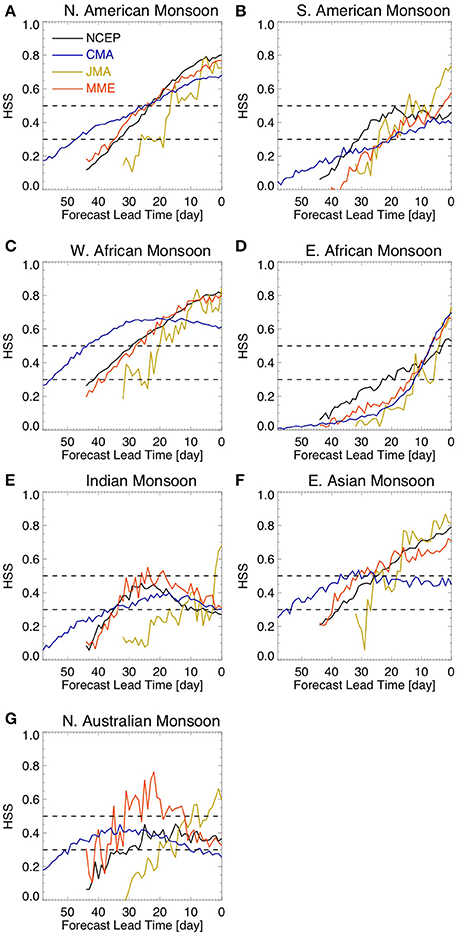
Figure 4. HSS for onset date hindcasts. The dashed lines show HSS equal to 0.3 and 0.5. The figure shows results for (A) North American Monsoon, (B) South American Monsoon, (C) West African Monsoon, (D) East African Monsoon, (E) Indian Monsoon, (F) East Asian Monsoon, and (G) Northern Australian Monsoon. Lead-time 0 (zero) refers to the observed onset date.

Why are the hindcasts of onset dates not skillful over East Africa and India? The onset over these regions has relatively low variability relative to the other monsoon regions (Figures 3D–E); therefore it is more difficult to distinguish them from the noise in the system. Since we are using the climatology as the benchmark for measuring forecast skill, the lower the amplitude of the onset dates the closer they are to climatology and, therefore, the more difficult it is to distinguish them from climatology.

To demonstrate the evolution of the onset forecast errors we calculated the ratio between the mean square error of onset hindcasts and the mean square error using the climatology as predictor for every year and every lead-time. Figures 5, 6 show the results for the South American (Figure 5) and Indian (Figure 6) monsoon regions, respectively. South America is an example of a region where the onset date shows high predictability. The MME and NCEP hindcasts outperform the climatology by 24–45 days (Figures 5a,b). Likewise, with the exception of a few years the CMA hindcasts outperform the observed climatology by more than 30 days (Figure 5c). In contrast, the Indian monsoon is a region where the models show little improvement over the climatology. NCEP and CMA could only outperform the climatology for some years and only for a lead-time window that ends sometime prior to the observed onset date (Figure 6). Due to the fact that JMA (Figures 5d, 6D) hindcast members were initialized in sets of simulations with an interval of approximately 10 days (Table 1) the forecast errors of these hindcasts are much less consistent than those from NCEP (Figures 5b, 6B) and CMA (Figures 5c, 6C).

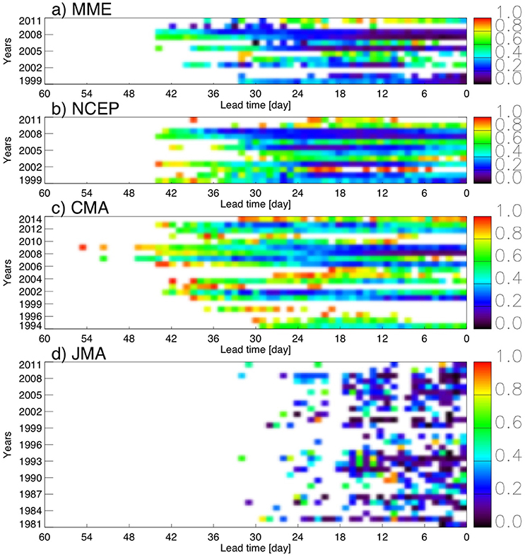
Figure 5. Lead-time ratio between the simulated mean squared error of onset dates and the onset mean square error using the climatology as predictor. The figure shows the results for the (a) MME; (b) NCEP, (c) CMA, and (d) JMA models over the South American monsoon region. Lead-time 0 (zero) refers to the observed onset date. The shading only shows values where the hindcasts outperform the climatology and are statistically significant at 5% level according to an f-test of the squared errors.

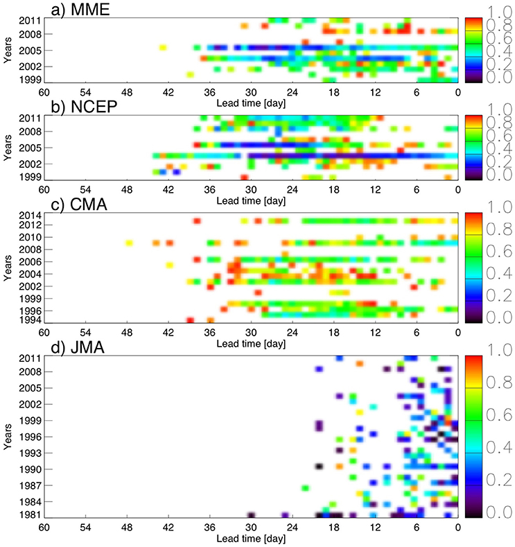
Figure 6. As in Figure 5 but for the Indian monsoon region.

In order to present a global view of the onset forecast error, Figure 7 shows the ratio between the mean squared error of simulated onset dates for lead-times during week 4 and the mean squared error calculated using the climatology as predictor. There is a remarkable similarity between models. If we focus on the two more reliable sets of simulations, NCEP (Figure 7A) and CMA (Figure 7B), we notice that the models outperform the climatology over most of South America, West Africa, and the Sahel region, East Asia, and northern Australia. At lead-times during week 4 the climatology outperforms the models over the western flank of North America, East Africa, India, and western China (Figure 7). These results correspond well to the map of onset date variability (Figure 2B) and are consistent with the notion that regions with relatively low onset date variance are regions that show the lowest forecast skill relative to climatology. It is important to mention that when these same analyses (Figure 7) are performed with the TRMM precipitation dataset, the results are consistent almost everywhere except over Africa (not shown). Results over Africa should be interpreted carefully due to the scarcity of observed precipitation data.

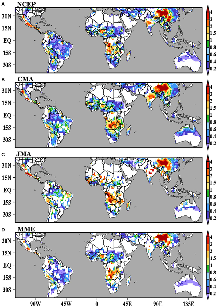
Figure 7. Ratio between the mean squared error of simulated onset dates for lead-times during week 4 and the mean squared error calculated using the climatology as predictor. The figure shows the results for (A) NCEP, (B) CMA, (C) JMA, and (D) MME. We mask regions where explained variance of the first harmonic of the mean annual cycle of observed precipitation is small (<30%). Shading indicates the squared errors are statistically different at 5% level according to an f-test.

The Demise of the Rainy Season

Demise Date Climatology

The latitudinal variation of the demise dates of the rainy season also reflects the seasonal evolution of convection, with the end of the rainy season usually occurring during the fall in each hemisphere (Figure 8A). Similar to the onset dates (Figure 2B), the western flank of the North American and Indian monsoon regions show low variability of demise dates (Figure 8B). In contrast to the onset dates (Figure 2B), the demise dates show less variability over the West African monsoon region than over the East African region (Figure 8B).

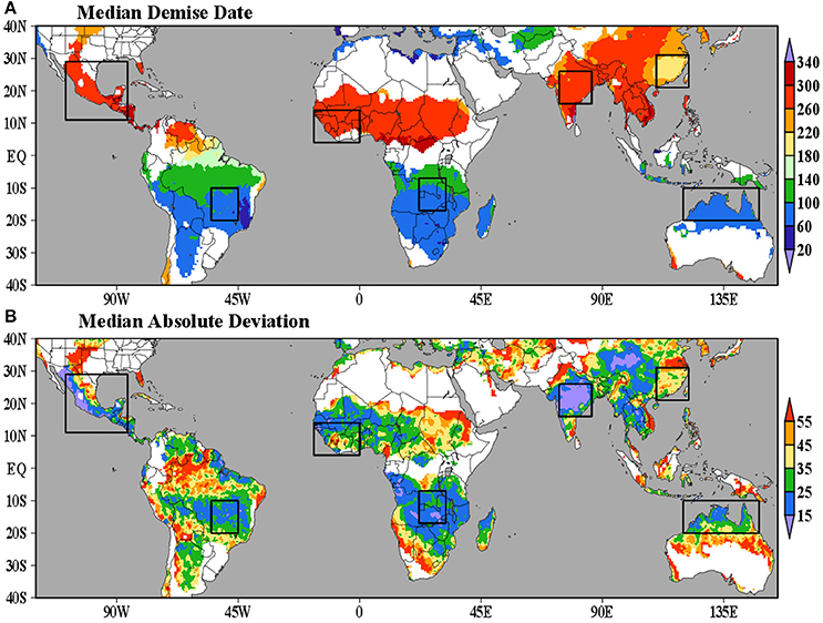
Figure 8. (A) Median demise date [DOY or Julian day] and (B) Interquartile range of demise dates calculated from CPC_UNI data (1979–2014). The boxes indicate monsoonal regions of interest. We mask regions where explained variance of the first harmonic of the mean annual cycle of observed precipitation is small (<30%).

Demise Date Hindcasts

All three models outperform the climatology by at least 25 days lead-time over all monsoon regions considered (Figure 9). The regions that show the smallest demise date forecast error (Figure 9) do not necessarily coincide with the ones that have the smallest onset date forecast error (Figure 3). For instance, over West Africa (Figure 9C) the forecast of the demise date is not as skillful as the forecast of the onset date (Figure 3C). In contrast, the forecast of the demise date over India (Figure 9E) is much more skillful than the forecast of the onset date (Figure 3E), consistent with the fact that the demise date of the Indian monsoon is more variable than its onset date (Syroka and Toumi, 2004).

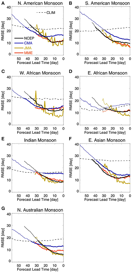
Figure 9. Lead-time RMSE of rainy season demise date forecasts. The figure shows results for (A) North American Monsoon, (B) South American Monsoon, (C) West African Monsoon, (D) East African Monsoon, (E) Indian Monsoon, (F) East Asian Monsoon, and (G) Northern Australian Monsoon. Lead-time 0 (zero) refers to the observed demise date. Thick lines show lead times where the RMSE of hindcasts is smaller than the RMSE related to the climatology and their difference is statistically significant at 5% level according to an f-test of the squared errors. The dashed line shows the RMSE in relation to the climatology for the CMA model grid for the sole purpose of visualization.

In terms of forecast skill, the regions that show the most consistency among the models are South America (Figure 10B), East Asia (Figure 10F), and Northern Australia (Figure 10G). There is less consistency among the models over North America (Figure 10A), West Africa (Figure 10C), East Africa (Figure 10D), and India (Figure 10E). However, the NCEP model shows a consistent increase in forecast skill as the lead-time approaches the observed demise date for all monsoon regions considered, with HSS above 0.3 at least a month in advance (Figure 10). These results are consistent with the forecast error (Figure 9), suggesting that the demise of the rainy season over most monsoonal regions is predictable in current models on sub-seasonal scales.

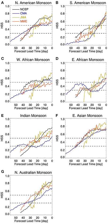
Figure 10. HSS for onset date hindcasts. The dashed lines show HSS equal to 0.3 and 0.5. The figure shows results for (A) North American Monsoon, (B) South American Monsoon, (C) West African Monsoon, (D) East African Monsoon, (E) Indian Monsoon, (F) East Asian Monsoon, and (G) Northern Australian Monsoon. Lead-time 0 (zero) refers to the observed onset date.

To evaluate demise date forecast error for the global monsoon, Figure 11 shows the ratio between the mean squared error of simulated demise dates for lead-times during week 4 and the mean squared error calculated using the climatology as predictor. Considering only the two more reliable sets of simulations, NCEP (Figure 11A) and CMA (Figure 11B), the models outperform the climatology over most of South America, East Asia, and Northern Australia. The climatology outperforms the models over parts of South America, most of the African Sahel, and India. The NCEP model outperforms the climatology over most of East Africa (Figure 11A) while the climatology outperforms CMA over East Africa and Madagascar (Figure 11B). These results correspond well to the map of demise date variability (Figure 8B) and are consistent with the notion that regions with relatively low demise date variance are regions that show the lowest relative forecast skill. The demise results are also consistent when the same analyses (Figure 11) are performed with the TRMM precipitation dataset, with exception of Africa (not shown). As with onset, results over Africa should be interpreted carefully due to the scarcity of precipitation observations.

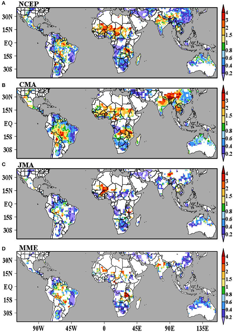
Figure 11. Ratio between the mean squared error of simulated demise dates for lead-times during week 4 and the mean squared error calculated using the climatology as predictor. The figure shows the results for (A) NCEP, (B) CMA, (C) JMA, and (D) MME. We mask regions where explained variance of the first harmonic of the mean annual cycle of observed precipitation is small (<30%). Shading indicates the squared errors are statistically different at 5% level according to an f-test.

Precipitation Bias and Time Series Discontinuity

This section explores the role of model precipitation bias and discontinuities in the time series of precipitation on the predictability of the onset and demise dates of the rainy season. Since we used a combination of observed and simulated precipitation to forecast the onset and demise dates of the rainy season, precipitation bias and discontinuities in the time series might play a role in the perceived predictability. For brevity, we will only focus on the MME results in this section.

We start by analyzing simulated precipitation bias. Figure 12 presents the MME precipitation bias for lead-times of 1, 2, 3, and 4 weeks for hindcasts initialized close to the observed onset (Figures 12A–D) and demise (Figures 12E–H) dates of the rainy season (i.e., all hindcasts with predictions of the observed onset or demise date of the rainy season). Most regions show positive precipitation biases around the onset date, except for South America, India, parts of East Asia, and northern Australia, which show negative precipitation biases in the first 2–3 weeks of the hindcasts (Figures 12A–D). Most regions show positive precipitation biases around the demise date as well, except for northern South America (Figures 12E–H).

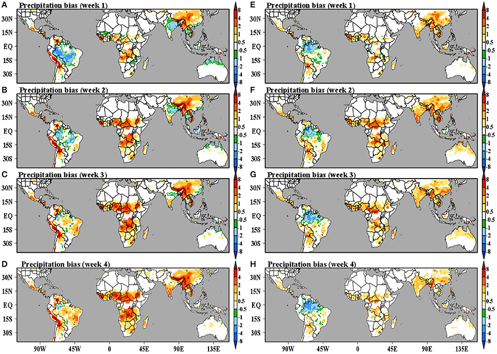
Figure 12. Precipitation bias [mm/day] around the time of the onset (left) and demise (right) of the rainy season for simulation lead-times within week 1 (A,E), 2 (B,F), 3 (C,G), and 4 (D,H). We mask regions where explained variance of the first harmonic of the mean annual cycle of observed precipitation is small (<30%).

We now compare the behavior of the S curve (Equation 1, Figure 1) between observations and hindcasts. Figure 13 shows the S curve for both observations and hindcasts spatially averaged over the monsoonal regions of interest. The S curve was also averaged over simulations with lead times of up to 4 weeks (28 days) in relation to the observed onset or demise date of the rainy season. It is important to note that these are relatively large regions and long lead-times. For the onset of the rainy season, we find that regions where the simulated precipitation shows positive bias are regions where the inflection in the S curve (Equation 1; Figure 1) happens earlier in the hindcasts than in the observations (Figures 13A,C,D). In contrast, the S curve for places like South America, East Asian, India, and northern Australia (Figures 13B,E,F,G) experience a late inflection in the hindcasts compared to the observations, corresponding to a negative precipitation bias. We find a similar correspondence of early versus late inflection of the S curve associated with positive and negative precipitation bias in the demise dates of the rainy season, but not as pronounced as in the onset dates (Figures 13H–N). Since the S curve consists of accumulated precipitation anomalies, the main impact of precipitation bias is simply to change the rate of change of S. Given that the S curve is smoothed prior to the calculation of the onset and demise dates the effect of the discontinuity between the time series of observed and simulated precipitation also contributes only to change the rate of change of S.

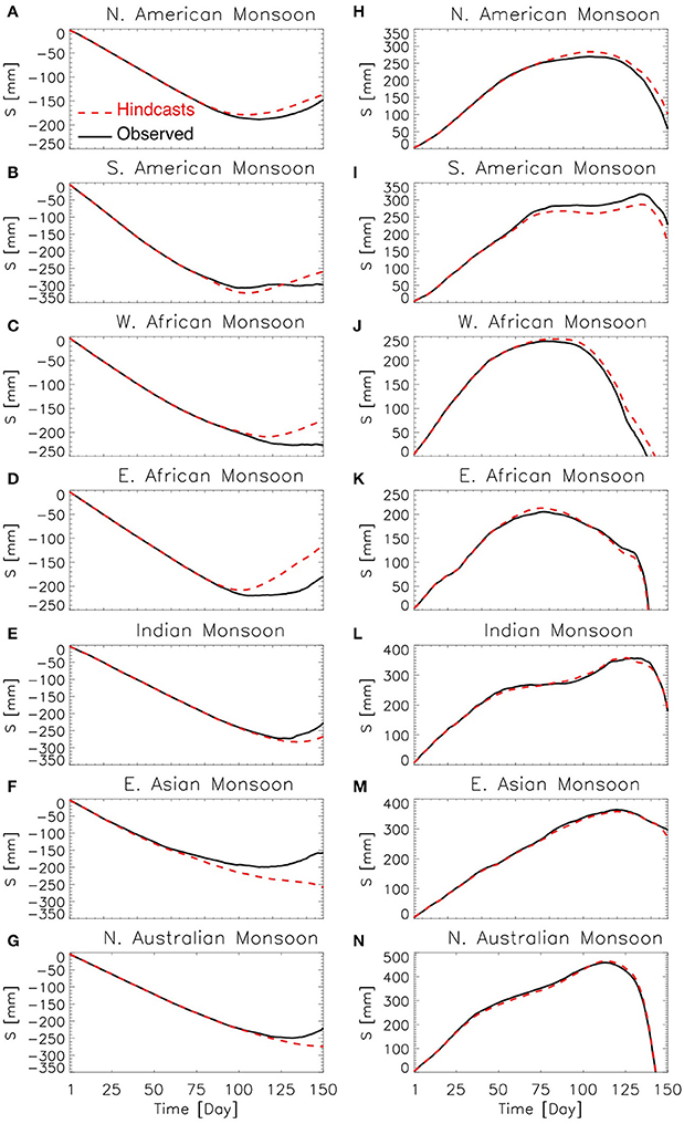
Figure 13. Observed (solid) and simulated (dashed) S curve [mm] for the onset (left) and the demise (right) of the rainy season. The figure shows results for (A,H) North American Monsoon, (B,I) South American Monsoon, (C,J) West African Monsoon, (D,K) East African Monsoon, (E,L) Indian Monsoon, (F,M) East Asian Monsoon, and (G,N) Northern Australian Monsoon. The S curve was spatially averaged over the monsoonal regions of interest and averaged over all hindcasts initialized up to 4 weeks before the observed onset or demise dates. Note y-axis.

Conclusions and Discussions

In this work we evaluated the retrospective forecasts of three global coupled models participating in the S2S project. We show that the onset and demise dates of the rainy season over several monsoonal regions can be skillfully forecasted on sub-seasonal timescales. South America, East Asia, and Northern Australia are monsoonal regions where we find that skillful forecasts for the onset date exists as much as 1 month in advance. On the other hand, the Indian monsoon region shows low forecast skill for the onset date. The demise dates show sub-seasonal forecast skill over parts of North and South America, East Asia, and Northern Australia as much as 1 month in advance. The NCEP model also shows good demise date forecast skill over the Indian monsoon region by at least 3 weeks. The forecast skill for the onset and the demise dates over East Africa, West Africa, and the African Sahel should be interpreted with caution due to the scarcity of in-situ precipitation observations in these regions.

Consistent daily model initializations are crucial for the proper evaluation of lead-time forecast skill of the onset and demise dates of the rainy season. Onset and demise dates vary seasonally from region to region and long intervals between initializations (such as 10 days in the JMA hindcasts) can have a large impact in the detection of the simulated onset or demise dates over certain regions.

This method for predicting the onset and demise dates of the monsoons is relatively simple since it depends only on precipitation data. Although skillful model precipitation predictions remain challenging in many regions, we have demonstrated that (when combined in a hybrid approach) they are skillful enough to identify onset and demise dates of the rainy season in many monsoon regions at sub-seasonal lead-times in retrospective forecasts of current operational models.

Another advantage of our method is the fact that the characteristics of the rainy season can be determined over every grid point, providing the user with information at higher spatial resolution than methods using large-scale indices for monsoon prediction. It is worth mentioning that the representation of the rainy season does not guarantee an accurate representation of a monsoon system as a whole (Soman and Kumar, 1993; Joseph et al., 1994) since monsoons are complex large-scale phenomena. However, our method provides information that can be used at the local level.

The combination of observations and model predictions in the calculation of the onset and demise dates provides a practical hybrid methodology for predicting monsoon onset and demise over the model or observations alone, since the predictions are of a cumulative quantity rather than a single arbitrary event. However, this could create a challenge for real-time predictions in regions where real-time quality controlled precipitation observations are scarce, but could be a useful methodology in well-observed regions.

This method works well for regions with precipitation regimes composed of a single well-defined rainy and dry season per year (Bombardi and Carvalho, 2008, 2009) and is thus most suitable for tropical monsoonal regions. For regions with two rainy seasons, such as some equatorial regions, the method is slightly less accurate as it tends to capture the most predominant rainy season. This method is the least accurate for regions without a well-defined rainy and dry season, such as most mid-latitude regions.

Since our method can provide detailed (at every grid point) forecasts of the onset and demise dates of the rainy season, it is a useful tool for providing information to decision makers. This is especially true when combined with methods that can provide forecasts for the large-scale aspect of monsoons, such as statistical methods (e.g., Moron et al., 2009a,b; Stolbova et al., 2016), dynamic prediction of monsoon indexes (e.g., Vellinga et al., 2013; Alessandri et al., 2015), and even the integration of statistical and dynamical prediction (e.g., Coelho et al., 2006).

Author Contributions

RB experiment design, data analysis, and manuscript writing. KP critical revision and scientific advising. JK fund-raising and scientific advising. BC data acquisition and scientific advising. JA data acquisition, formatting, and organizing.

Conflict of Interest Statement

The authors declare that the research was conducted in the absence of any commercial or financial relationships that could be construed as a potential conflict of interest.

The reviewer NA and handling Editor declared their shared affiliation, and the handling Editor states that the process nevertheless met the standards of a fair and objective review.

Acknowledgments

This study is supported by NSF (AGS-1338427), NOAA (NA14OAR4310160 and NA15NWS4680018), and NASA (NNX14AM19G). In addition, we thank NOAA Climate Prediction Center for making available the CPC Unified Gauge-Based Analysis of Global Daily Precipitation and the National Aeronautics and Space Administration for making available the TRMM analysis. We thank Dr. Brant Liebmann and the three other anonymous reviewers for their suggestions for the improvement of this manuscript.

References

Appendix

Forecast Error and Skill Using Ensemble Means and TRMM Data

We also investigated the results shown in Figures 3, 4 using TRMM data and ensemble means (Figures A1, A2). We calculated two different ensembles: Ensemble 1 (ENS) was calculated by computing the ensemble mean of daily precipitation prior to the calculation of the onset and demise dates. Ensemble 2 (ENS 2) was calculated by first calculating the onset and demise dates and then calculating the ensemble average. Ensemble 1 and 2 were calculated with CPC_UNI data. The ensemble means are slightly more skillful than considering all the hindcast members individually. All results presented in this appendix were calculated using the NCEP hindcasts.

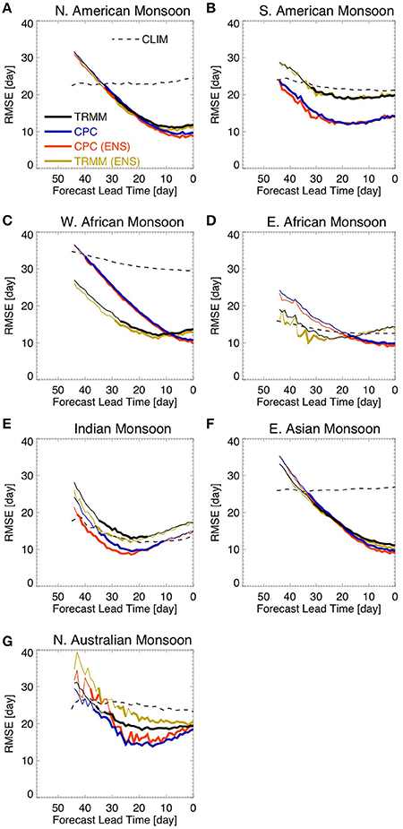
Figure A1. Lead-time RMSE of rainy season onset date forecasts. The figure shows results for (A) North American Monsoon, (B) South American Monsoon, (C) West African Monsoon, (D) East African Monsoon, (E) Indian Monsoon, (F) East Asian Monsoon, and (G) Northern Australian Monsoon. Lead-time 0 (zero) refers to the observed onset date. Thick lines show lead times where the RMSE of hindcasts is smaller than the RMSE related to the climatology and their difference is statistically significant at 5% level according to an f-test of the squared errors. The dashed line shows the RMSE in relation to the climatology for the NCEP model grid for the sole purpose of visualization.

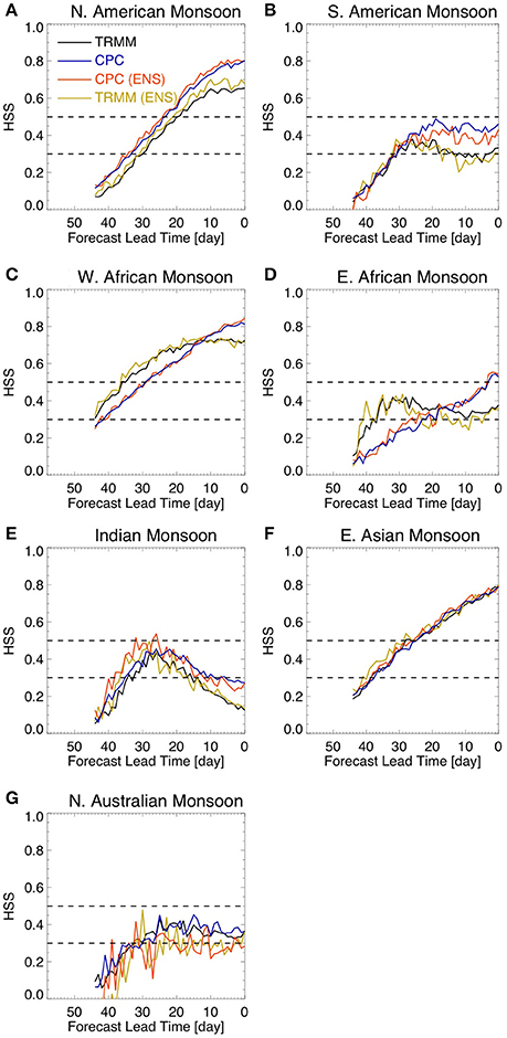
Figure A2. HSS for onset date hindcasts. The dashed lines show HSS equal to 0.3 and 0.5. The figure shows results for (A) North American Monsoon, (B) South American Monsoon, (C) West African Monsoon, (D) East African Monsoon, (E) Indian Monsoon, (F) East Asian Monsoon, and (G) Northern Australian Monsoon. Lead-time 0 (zero) refers to the observed onset date.

The results using CPC_UNI data, TRMM data, and ensemble means are very similar to the results presented in Figures 3, 4 (Figures A1, A2, respectively). Although there are differences in forecast error and forecast skill of onset dates between results using CPC_UNI data and results using TRMM data, these differences are usually small. However, some regions show larger differences (e.g., West Africa and South America) than others.

Regarding the forecast of the rainy season demise, when we consider TRMM data or ensemble means the results are very similar to the results presented in Figures 9, 10 (no shown). Although there are differences in forecast error and forecast skill of demise dates between results using CPC_UNI data and results using TRMM data, these differences are usually small. However, some regions show larger differences (e.g., North America, West Africa, and India) than others.

References

Adams, D. K., and Comrie, A. C. (1997). The North American monsoon. Bull. Am. Meteorol. Soc. 78, 2197–2213. doi: 10.1175/1520-0477(1997)078<2197:TNAM>2.0.CO;2
Alessandri, A., Borrelli, A., Cherchi, A., Materia, S., Navarra, A., Lee, J.-Y., et al. (2015). Prediction of Indian summer monsoon onset using dynamical subseasonal forecasts: effects of realistic initialization of the atmosphere. Mon. Weather Rev. 143, 778–793. doi: 10.1175/MWR-D-14-00187.1
Bombardi, R. J., and Carvalho, L. M. V. (2008). Variability of the monsoon regime over the Brazilian Savanna: the present climate and projections for a 2xCO2 scenario using the MIROC model. Rev. Bras. Meteorol. 23, 58–72. doi: 10.1590/S0102-77862008000100007
Bombardi, R. J., and Carvalho, L. M. V. (2009). IPCC global coupled model simulations of the South America monsoon system. Clim. Dyn. 33, 893–916. doi: 10.1007/s00382-008-0488-1
Bombardi, R. J., Schneider, E. K., Marx, L., Halder, S., Singh, B., Tawfik, A. B., et al. (2015). Improvements in the representation of the Indian summer monsoon in the NCEP climate forecast system version 2. Clim. Dyn. 45, 2485–2498. doi: 10.1007/s00382-015-2484-6
Bombardi, R. J., Tawfik, A. B., Manganello, J. V., Marx, L., Shin, C.-S., Halder, S., et al. (2016). The heated condensation framework as a convective trigger in the NCEP Climate Forecast System version 2. J. Adv. Model. Earth Syst. 8, 1310–1329. doi: 10.1002/2016MS000668
Carvalho, L. M. V., and Cavalcanti, I. F. A. (2016). The South American Monsoon System (SAMS). Springer International Publishing.
Charney, J. G., and Shukla, J. (1982). “Predictability of Monsoons,” in Monsoon Dynamics, eds L. James and R. P. Pearce (Cambridge; New York, NY: Cambridge University Press), 99–109.
Chen, M., Shi, W., Xie, P., Silva, V. B. S., Kousky, V. E., Wayne Higgins, R., et al. (2008). Assessing objective techniques for gauge-based analyses of global daily precipitation. J. Geophys. Res. 113:D04110. doi: 10.1029/2007jd009132
Cherchi, A., and Navarra, A. (2003). Reproducibility and predictability of the Asian summer monsoon in the ECHAM4-GCM. Clim. Dyn. 20, 365–379. doi: 10.1007/s00382-002-0280-6
Coelho, C. A. S., Stephenson, D. B., Balmaseda, M., Doblas-Reyes, F. J., and van Oldenborgh, G. J. (2006). Toward an integrated seasonal forecasting system for South America. J. Clim. 19, 3704–3721. doi: 10.1175/JCLI3801.1
Hendon, H. H., and Liebmann, B. (1990). A composite study of onset of the Australian summer monsoon. J. Atmos. Sci. 47, 2227–2240. doi: 10.1175/1520-0469(1990)047<2227:ACSOOO>2.0.CO;2
Huffman, G. J., Bolvin, D. T., Nelkin, E. J., Wolff, D. B., Adler, R. F., Gu, G., et al. (2007). The TRMM Multisatellite Precipitation Analysis (TMPA): quasi-global, multiyear, combined-sensor precipitation estimates at fine scales. J. Hydrometeorol. 8, 38–55. doi: 10.1175/JHM560.1
Joseph, P. V., Eischeid, J. K., and Pyle, R. J. (1994). Interannual variability of the onset of the Indian summer monsoon and its association with atmospheric features, El Ni-o, and sea surface temperature anomalies. J. Clim. 7, 81–105. doi: 10.1175/1520-0442(1994)007<0081:IVOTOO>2.0.CO;2
Krishnamurthy, V., and Shukla, J. (2000). Intraseasonal and interannual variability of rainfall over India. J. Clim. 13, 4366–4377. doi: 10.1175/1520-0442(2000)013<0001:IAIVOR>2.0.CO;2
Krishnamurthy, V., and Shukla, J. (2012). Predictability of the Indian monsoon in coupled general circulation models, Monographs. Government of India, Ministry of Earth Sciences, India Meteorological Department.
Li, J., and Zhang, L. (2009). Wind onset and withdrawal of Asian summer monsoon and their simulated performance in AMIP models. Clim. Dyn. 32, 935–968. doi: 10.1007/s00382-008-0465-8
Liebmann, B., and Marengo, J. A. (2001). Interannual variability of the rainy season and rainfall in the Brazilian amazon basin. J. Clim. 14, 4308–4318. doi: 10.1175/1520-0442(2001)014<4308:IVOTRS>2.0.CO;2
Mann, M. E. (2004). On smoothing potentially non-stationary climate time series. Geophys. Res. Lett. 31:L07214. doi: 10.1029/2004gl019569
Marengo, J. A., Liebmann, B., Grimm, A. M., Misra, V., Silva Dias, P. L., Cavalcanti, I. F. A., et al. (2012). Recent developments on the South American monsoon system. Int. J. Climatol. 32, 1–21. doi: 10.1002/joc.2254
Moron, V., Lucero, A., Hilario, F., Lyon, B., Robertson, A. W., and DeWitt, D. (2009a). Spatio-temporal variability and predictability of summer monsoon onset over the Philippines. Clim. Dyn. 33, 1159–1177. doi: 10.1007/s00382-008-0520-5
Moron, V., Robertson, A. W., and Boer, R. (2009b). Spatial coherence and seasonal predictability of monsoon onset over Indonesia. J. Clim. 22, 840–850. doi: 10.1175/2008JCLI2435.1
Mutai, C. C., and Ward, M. N. (2000). East African rainfall and the tropical circulation/convection on intraseasonal to interannual timescales. J. Clim. 13, 3915–3939. doi: 10.1175/1520-0442(2000)013<3915:EARATT>2.0.CO;2
Nairobi, N. (1979). The East African monsoons and their effects on agriculture. GeoJournal 3, 193–200. doi: 10.1007/BF00257708
Nicholson, S. E. (2013). The West African sahel: a review of recent studies on the rainfall regime and its interannual variability. ISRN Meteorol. 2013, 1–32. doi: 10.1155/2013/453521
Prasad, V. S. (2005). Onset and withdrawal of Indian summer monsoon. Geophys. Res. Lett. 32:L20715. doi: 10.1029/2005GL023269
Robertson, A. W., Kumar, A., Pe-a, M., and Vitart, F. (2015). Improving and promoting subseasonal to seasonal prediction. Bull. Am. Meteorol. Soc. 96, ES49–ES53. doi: 10.1175/bams-d-14-00139.1
Saha, S., Moorthi, S., Pan, H.-L., Wu, X., Wang, J., Nadiga, S., et al. (2010). The NCEP climate forecast system reanalysis. Bull. Am. Meteorol. Soc. 91, 1015–1057. doi: 10.1175/2010BAMS3001.1
Saha, S., Moorthi, S., Wu, X., Wang, J., Nadiga, S., Tripp, P., et al. (2014). The NCEP climate forecast system version 2. J. Clim. 27, 2185–2208. doi: 10.1175/JCLI-D-12-00823.1
Soman, M. K., and Kumar, K. K. (1993). Space-time evolution of meteorological features associated with the onset of Indian summer monsoon. Mon. Weather Rev. 121, 1177–1194. doi: 10.1175/1520-0493(1993)121<1177:STEOMF>2.0.CO;2
Stolbova, V., Surovyatkina, E., Bookhagen, B., and Kurths, J. (2016). Tipping elements of the Indian monsoon: prediction of onset and withdrawal. Geophys. Res. Lett. 43, 3982–3990. doi: 10.1002/2016GL068392
Syroka, J., and Toumi, R. (2004). On the withdrawal of the Indian summer monsoon. Q. J. R. Meteorol. Soc. 130, 989–1008. doi: 10.1256/qj.03.36
Vellinga, M., Arribas, A., and Graham, R. (2013). Seasonal forecasts for regional onset of the West African monsoon. Clim. Dyn. 40, 3047–3070. doi: 10.1007/s00382-012-1520-z
Vera, C., Higgins, W., Amador, J., Ambrizzi, T., Garreaud, R., Gochis, D., et al. (2006). Toward a unified view of the American monsoon systems. J. Clim. 19, 4977–5000. doi: 10.1175/JCLI3896.1
Wang, B., Lee, J.-Y., and Xiang, B. (2015). Asian summer monsoon rainfall predictability: a predictable mode analysis. Clim. Dyn. 44, 61–74. doi: 10.1007/s00382-014-2218-1
Wang, B., Wu, R., and Lau, K.-M. (2001). Interannual variability of the Asian summer monsoon: contrasts between the Indian and the Western North Pacific–East Asian Monsoons*. J. Clim. 14, 4073–4090. doi: 10.1175/1520-0442(2001)014<4073:IVOTAS>2.0.CO;2
Webster, P. J., Maga-a, V. O., Palmer, T. N., Shukla, J., Tomas, R. A., Yanai, M., et al. (1998). Monsoons: processes, predictability, and the prospects for prediction. J. Geophys. Res. Ocean. 103, 14451–14510. doi: 10.1029/97JC02719
Wilks, D. S. (2006). Statistical Methods in the Atmospheric Sciences. Burlington, MA: Academic Press.
Wu, T., Song, L., Li, W., Wang, Z., Zhang, H., Xin, X., et al. (2014). An overview of BCC climate system model development and application for climate change studies. Acta Meteorol. Sin. 28, 34–56. doi: 10.1007/s13351-014-3041-7
Wu, T., Yu, R., Zhang, F., Wang, Z., Dong, M., Wang, L., et al. (2010). The Beijing Climate Center atmospheric general circulation model: description and its performance for the present-day climate. Clim. Dyn. 34, 123–147. doi: 10.1007/s00382-008-0487-2
Xie, P., Chen, M., Yang, S., Yatagai, A., Hayasaka, T., Fukushima, Y., et al. (2007). A gauge-based analysis of daily precipitation over East Asia. J. Hydrometeorol. 8, 607–626. doi: 10.1175/JHM583.1
Yihui, D., and Chan, J. C. L. (2005). The East Asian summer monsoon: an overview. Meteorol. Atmos. Phys. 89, 117–142. doi: 10.1007/s00703-005-0125-z
Zhou, T., and Zou, L. (2010). Understanding the predictability of East Asian summer monsoon from the reproduction of land–sea thermal contrast change in AMIP-type simulation. J. Clim. 23, 6009–6026. doi: 10.1175/2010JCLI3546.1
Zuo, Z., Yang, S., Hu, Z.-Z., Zhang, R., Wang, W., Huang, B., et al. (2013). Predictable patterns and predictive skills of monsoon precipitation in Northern Hemisphere summer in NCEP CFSv2 reforecasts. Clim. Dyn. 40, 3071–3088. doi: 10.1007/s00382-013-1772-2