Traditional Calibration Methods in Atomic Spectrometry and New Calibration Strategies for Inductively Coupled Plasma Mass Spectrometry
 Jake A. Carter
 Ariane I. Barros
 Joaquim A. Nóbrega
 George L. Donati
- 1Department of Chemistry, Wake Forest University, Winston-Salem, NC, United States
- 2Group for Applied Instrumental Analysis, Department of Chemistry, Federal University of São Carlos, São Carlos, Brazil
Applications, advantages, and limitations of the traditional external standard calibration, matrix-matched calibration, internal standardization, and standard additions, as well as the non-traditional interference standard method, standard dilution analysis, multi-isotope calibration, and multispecies calibration methods are discussed.
Introduction
Instrumental spectrochemical methods are widely used in trace element analysis of all types of samples, and different calibration strategies such as external standard calibration (EC), matrix-matched calibration (MMC), internal standardization (IS), and standard additions (SA) are employed to overcome matrix effects and improve accuracy and precision. These traditional calibration methods are closely associated with several of the most commonly used spectroanalytical methods, as discussed here.
It is well-known that inductively coupled plasma mass spectrometry (ICP-MS) is severely affected by different interfering effects, and several strategies have been developed for overcoming them. In inductively coupled plasma optical emission spectrometry (ICP OES), non-spectral interferences can be related to transport effects during sample introduction, and plasma effects such as those caused by high concentrations of either carbon or easily-ionized elements. Interface processes, such as self-absorption in axial-viewing ICP OES, space charge effects in ICP-MS, and recombination processes in both ICP OES and ICP-MS, are also responsible for biased results. Spectral interferences are mainly related to processes involving nearby emission lines and background signals (ICP OES), isotopes with nearby masses (for the typical low-resolution quadrupole-based ICP-MS), double charge species (ICP-MS), and effects caused by polyatomic ions (ICP OES and ICP-MS). In quadrupole-based ICP-MS (ICP-QMS), these effects can be corrected by using specially designed instrumentation containing a collision/reaction cell (CRC) with a single quadrupole, or a tandem arrangement with two quadrupoles and a CRC. A simpler and cost-effective alternative to correct for interfering effects in both ICP OES and ICP-MS is the use of special strategies for calibration.
In this review paper, we discuss applications, advantages and limitations of traditional and non-traditional calibration methods. The discussions associated with the traditional calibration strategies involve several instrumental spectrochemical methods. On the other hand, the non-traditional calibration strategies examined here, which include the interference standard method (IFS), standard dilution analysis (SDA), multi-isotope calibration (MICal), and multispecies calibration (MSC), are focused on ICP-MS applications. All discussions are based on landmark papers and recent works describing the state of the art of new approaches. A careful reading of this literature suggests that several interfering effects can be controlled, without any instrument modification, by fully exploiting data acquisition and processing. Thus, simple calibration strategies may be able to improve accuracy and precision in trace element analysis.
Traditional Calibration Methods
The External Standard (EC) and Matrix-Matched Calibration (MMC) Methods
In analytical chemistry, calibration involves the determination of a mathematical function describing the relationship between analyte concentration and instrument response. A series of calibration standards is used to determine this function, which is then applied to determine the unknown amount of analyte in a sample (Currie, 1998; Cuadros-Rodríguez et al., 2001; AOAC International, 2002). Usually, calibration is performed in three steps: standard solution preparation, analytical signal measurement, and mathematical calculation (i.e., determination of the calibration function model; Kościelniak, 2003). The first step will depend on the type of calibration method used. The traditional EC, MMC, IS, and SA methods are the most commonly used calibration strategies, with broad application in quantitative analytical chemistry.
The EC method is the most straightforward, and therefore, the most used among the traditional calibration strategies. It is called external standard calibration because certified pure substances or standard solutions used in the calibration procedure are external to the sample. It assumes matrix effects are absent or have negligible impact on the analytical signal. In many applications, this is in fact the case, and EC can be successfully applied by simply comparing the analytical signals from standard solutions with those from samples. In principle, EC can be performed using single, double or multiple calibration standards (Cuadros-Rodríguez et al., 2001). However, better precision and accuracy are achieved by adopting a multiple-point calibration (Miller and Miller, 1984). In this case, a set of standard solutions are analyzed, and analyte concentration vs. instrument response are plotted as independent variable (x-axis) and dependent variable (y-axis), respectively. The analyte concentration in the sample can then be determined by interpolation using the mathematical function obtained from the calibration plot, which is usually determined using least-squares regression. The instrument response recorded for the sample is converted into analyte concentration using a relationship such as IR = a + bC, where IR, a, b, and C correspond to instrument response, y-intercept, slope, and analyte concentration, respectively (Cuadros-Rodríguez et al., 2001). It is recommended by the AOAC International (2002) that the analyte concentrations in the standard solutions should be close to the one in the sample, and that 6–8 standard concentrations should be used for calibration.
In EC, as well as in other strategies, the choice of the calibration model depends on the characteristics of the data obtained (Currie, 1998). Linearity (or linear dynamic range), for example, can be tested graphically by a residual plot, or numerically by a correlation coefficient (r). One can also apply different statistical tools to check for linearity such as, for instance, the F-test. When employing this statistical method, the ratio between residual standard deviations of the linear model and those of a non-linear model is determined. If F calculated (Fcal) is lower than F tabulated (Ftab, usually at a 95% confidence level), the model is considered linear. On the other hand, if Fcal > Ftab, a non-linear model (e.g., a quadratic model) should be used (Currie, 1998; Mermet, 2010; Raposo, 2016).
Ordinary least-squares (OLS) is a linear model based on minimization of the sum of squares of deviations (i.e., the difference between expected values and experimental data; Currie, 1998; Mermet, 2010). It can only be applied when variables are normally distributed, the error in concentration values (independent variable) is minimal when compared with the analytical signal error (dependent variable), and when the data are homoscedastic (Mermet, 2010). Homoscedasticity occurs when a sequence of random data presents homogeneous variance. To evaluate whether variations are homogeneous, statistical methods such as the Hartley and Bartlett test (Currie, 1998) are commonly employed. In most cases, data obtained from consolidated spectroanalytical instrumental methods are normally distributed and homoscedastic, and errors in standard solution concentrations are negligible, hence the OLS approach can be successfully applied in conjunction with EC.
Heteroscedasticity occurs when variances are heterogeneous, in which case OLS cannot be applied, and alternative models such as the weighted least-squares (WLS) must be used (Currie, 1998; Mermet, 2010). Different from OLS, in which all calibration points have equal weights, lower-concentration standards have the highest weights in WLS, which results in increased accuracy for those calibration points. As discussed by Taylor and Schutyser (1986), the analyst needs to be thoughtful and know which calibration model the software of an instrument is using to avoid inaccurate results.
In elemental analyses by ICP OES, ICP-MS, flame atomic absorption spectrometry (F AAS), and graphite furnace atomic absorption spectrometry (GF AAS), it is frequently necessary to prepare the sample in a manner that makes it compatible with the sample introduction system. Ideally, samples are converted into a solution, with minimal or no matrix present, so EC can be successfully used. The EC method has been effective in several analytical applications involving elemental determination in different types of the matrices, such as crude oils (Trevelin et al., 2016; Sugiyama and Williams-Jones, 2018), diesel oil (Nora et al., 2017), biodiesel (Barros et al., 2017), iron supplements (Barbosa et al., 2015), vinegar alcohol (Silva Junior et al., 2015), sediment (Leao et al., 2016b), milk (Oliveira et al., 2017), canned foods (Leao et al., 2016a), seawater, mineral water, tap water, cachaça, human blood (Papai et al., 2017), among others. In these applications, acid digestion (Barbosa et al., 2015; Leao et al., 2016a; Sugiyama and Williams-Jones, 2018), dry decomposition (Nora et al., 2017), extraction procedures (Silva Junior et al., 2015; Leao et al., 2016b; Sánchez et al., 2016; Trevelin et al., 2016; Barros et al., 2017; Papai et al., 2017; Zeiner et al., 2018), and emulsion formation (Oliveira et al., 2017) were used for sample preparation. Table 1 shows a summary and additional details on sample preparation procedures used in combination with EC, as well as with MMC.
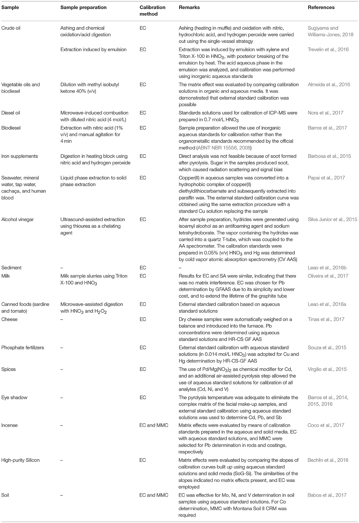
Table 1. Sample preparation procedures and direct sample analysis used in combination with EC or MMC in elemental determinations.
In addition to the procedures mentioned before, there are other types of sample preparation which are also compatible with EC. For example, dilution of biodiesel with ethanol allows for using inorganic standards and aqueous solutions in elemental determination by microwave-induced plasma optical emission spectrometry (MIP OES) and EC (Amais et al., 2013). Dilution of biodiesel and vegetable oil with isobutyl ketone is also compatible with EC using aqueous standards and determination by high resolution-continuum source GF AAS (HR-CS GF AAS; Almeida et al., 2016). Photo-oxidation by UV radiation is another strategy to minimize matrix effects and allow for using inorganic-matrix aqueous standard solutions in fruit juice analysis by F AAS and EC (Brandão et al., 2012). When possible, simple dilution of aqueous samples makes the application of EC even more straightforward. Zhuravlev et al. (2016), for example, employed EC in elemental analysis of ground natural water with moderate salinity (6.79 g/L) after a 10-fold dilution with 5% (v/v) HNO3. For samples with high salinity (16.8, 34.8 g/L), 20-fold dilutions in 5% (v/v) HNO3 were employed, and analyte concentrations were determined by filter-furnace electrothermal atomic absorption spectroscopy (FF ET-AAS). For determinations using inductively coupled plasma sector field mass spectrometry (ICP-SFMS) and ICP-QMS, a 10-fold dilution was sufficient for all samples. For more complex matrices, an alternative to simple dilution or total digestion is the use extraction procedures. Veguería et al. (2013), for example, used EC and ICP-MS for seawater analysis after preconcentration and matrix elimination on iminodiacetate resins and elution with nitric acid.
Direct solid sampling and HR-CS GF AAS determination using aqueous standard solutions and EC may significantly improve sample throughput, as minimal sample preparation is required. As examples of such a strategy we have elemental analysis of cheese (Tinas et al., 2017), fertilizers (Souza et al., 2015), spices (Virgilio et al., 2015), eye shadow (Barros et al., 2014, 2015, 2016), incense (Coco et al., 2017), high-purity silicon (Bechlin et al., 2016), and soil (Babos et al., 2017; Table 1).
Although widely used due to its simplicity and flexibility, EC frequently provides inaccurate results when applied to complex-matrix sample analyses. In these cases, methods such as SA may be more appropriate to minimize signal bias and improve accuracy, as will be discussed in detail in the following sections. Li et al. (2016), for example, reported poor accuracy in honey analysis by electrothermal vaporization ICP-MS (ETV-ICP-MS), which was caused by sample transport differences between the honey homogenate and standard solutions, and by non-spectral interferences (matrix effects). The honey suspension was prepared by dissolution with ascorbic acid and HNO3 and homogenation in an ultrasonic bath. Isotope dilution and SA were then successfully used for Cr, Cd, Hg, and Pb quantification (additional examples of the use of SA will be presented in its specific section later on the text). Borno et al. (2015) used EC for elemental determination in low-density polyethylene by ETV-ICP OES. However, for quantification of the analytes in acrylonitrile butadiene styrene copolymer, the ETV heating program was not efficient at decomposing the organic matrix, which compromised the method's accuracy. As expected, EC is ineffective when differences in matrix between calibration standard solutions and samples become significant. Even when total digestion is employed for sample preparation, differences in physical and chemical properties, such as pH, viscosity, ionic strength, temperature, and surface tension can lead to poor accuracies in EC determinations (Bader, 1980).
An alternative to SA for compensating for matrix effects in elemental analyses is the use of MMC. In this method, the matrix of the calibration standard solutions mimic that of the samples. If the constitution of both calibration standards and samples closely match, negligible matrix effects are expected. MMC is normally accomplished by adding certified reference materials (CRMs) to the calibration standards in direct solid analyses, or by adding interference-causing concomitants to the standard solutions at concentrations close to the ones found in the sample solution. As an example, MMC with aqueous standard solutions prepared in 5% v/v formic acid was used for simultaneous elemental determination by ETV-ICP-MS in biological samples, which were previously prepared by formic acid solubilization (Tormen et al., 2012). In another work, Sánchez et al. (2016) used MMC to minimize matrix effects in ICP-MS analysis using a total sample consumption nebulizer. Inorganic standards prepared in a 1:1 (v/v) mix of ethanol and water were used for the direct analysis of a bioethanol sample diluted with water at the same proportion.
Many other works using MMC can be found in the literature. Exoskeleton of clams was analyzed by energy dispersive X-ray fluorescence (EDX) using five CRMs of bone ash, and bovine and caprine bone as calibration standards for MMC (Pessanha et al., 2018). Babos et al. (2018) also used MMC for Ca determination in mineral supplements for cattle by wavelength dispersive X-ray fluorescence (WD-XRF). In this case, a reference material of mineral supplements for cattle was diluted in solid phase with a Na2CO3:NaCl mixture. Rietig and Acker (2017) used MMC for trace element determination in a silicon sample previously digested with a mixture of HNO3 and HF. The standard solutions were matrix-matched by adding Si at levels similar to those expected for the sample solutions. In another work, Nunes et al. used filter paper embedded with reference solution as a solid standard for multielement analysis of botanical samples by ICP-MS coupled with laser ablation (LA; Nunes et al., 2016). The authors argue that filter paper presents similarities in composition with botanical materials, which makes it a good matrix-matching material for MMC.
Different from the procedure described by Amais et al. (2013) for MIP OES determinations, poor accuracies were obtained when using aqueous standard solutions and EC for elemental analysis of biodiesel samples dissolved in ethanol by both F AAS and flame atomic emission spectrometry (F AES). Alternatively, MMC using standard solutions prepared in washed biodiesel:ethanol at 1:20 v/v (Barros et al., 2012), or 1:10 v/v (Magalhães et al., 2014) resulted in adequate recoveries for F AES and F AAS determinations, respectively. The use of washed samples (i.e., biodiesel free of the analytes) for adjusting the viscosity of the standard solutions and matching it as close as possible to that of the samples has been proposed, in these cases, as an alternative to the use of mineral oils, which is recommended in the standard method ABNT NBR 15556 (2008).
Although efficient in some cases, MMC is difficult and cumbersome, as it becomes almost impossible to match the composition of more complex samples. Standard solutions usually have more than one property which is different from the samples', which frequently results in severe matrix effects despite the use of MMC (Cuadros-Rodríguez et al., 2001). Such differences can cause transport-related interferences during sample introduction in ICP OES, ICP-MS and F AAS. In laser-induced breakdown spectroscopy (LIBS), inhomogeneous interaction between laser and sample matrix causes variation in signal intensities, which frequently compromises repeatability and accuracy (Singh and Thakur, 2007). In addition, matrix differences between calibration standards and samples can result in different mechanisms of atomization, excitation and ionization taking place in plasmas and flames, or in different mechanisms of atomization in GF AAS. In many cases, and especially due to the complexity of some sample matrices, MMC is not capable of minimizing such effects. The traditional alternatives to correct for these interferences include IS and SA, as we will discuss in the following sections.
Internal Standardization (IS)
Internal standardization, previously known as reference element technique, was proposed by Gerlach and Schweitezer (1929) to correct for interferences in atomic spectrometry. It consists of adding a reference element called internal standard (IS) to all samples, calibrations standards and the analytical blank, and using the analyte-to-IS signal ratio for calibration. The IS species has a known concentration, and ideally should be affected by the same processes as the analyte during the instrumental measurement. Thus, if the IS signal behaves similarly to the analyte's, their ratio should be relatively constant, which then minimizes the effects of fluctuations due to nebulization, radiation source intensity, sample position, or other instrumental parameters on accuracy. Although generally ineffective for minimizing matrix effects, the IS method may be used to that end in certain instances. The IS calibration curve is built by plotting the analyte concentration on the x-axis (independent variable), with the analyte/IS signal ratio on the y-axis (dependent variable).
The IS method requires that signals from both the analyte and IS species are monitored simultaneously, or at least fast sequentially, during the analysis. Therefore, it has been mainly used in multi-element methods such as ICP OES, ICP-MS, and LIBS, with limited applications in F AAS and GF AAS (Welz and Sperling, 1998). In F AAS, the development of dual-channel instruments allowed the use of IS to correct for variations in the sample introduction system, as reviewed by Fernandes et al. (2003). It has also been employed in elemental determinations using multi-channel GF AAS (Takada and Nakano, 1981). The development of graphite furnace simultaneous atomic absorption spectrometry (commercially named SIM AAS) and fast-sequential flame instruments contributed to increasing the number of applications involving the IS method in atomic absorption spectrometry (Radziuk et al., 1999; Fernandes et al., 2002; Correia et al., 2004; Oliveira et al., 2004, 2005; Oliveira and Gomes Neto, 2007; Ferreira et al., 2008a,b; Miranda et al., 2010; Caldas and Sanches Filho, 2013; Barkonikos et al., 2014; Pasias et al., 2014; Pereira et al., 2014). More recently, such applications have been further extended with the combination of an efficient continuum source, a high-resolution Echelle polychromator, and solid-state detectors in high-resolution continuum source F AAS (HR-CS F AAS) and HR-CS GF AAS. Fast-sequential analysis can be easily carried out with these instruments (Raposo et al., 2008, 2012), and simultaneous determinations are also possible when analytical and IS lines appear in the same spectral window (Babos et al., 2016).
Choosing the ideal IS species usually follows two main criteria: (i) analyte (A) and IS signals should have similar intensities, with A/IS as close as possible to unity, and (ii) the physicochemical properties of both A and IS should be as similar as possible to insure they undergo the same processes during analysis (Barnett, 1968; Barnett et al., 1970; Fernandes et al., 2003). The most critical properties of an IS species will depend on the instrumental method used. According to Walsh (1992), the ideal IS should be present in a non-detectable concentration in the sample, should have low toxicity and low cost, should not form insoluble compounds, and should have an appropriate spectral line with no spectral interferences of its own. Table 2 shows some examples of applications using the IS method, and describes the selection criteria adopted for choosing a suitable IS species in each case.
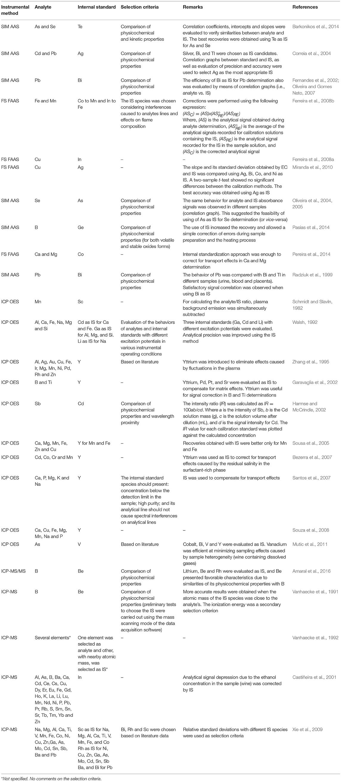
Table 2. Internal standardization applied to SIM AAS, FS FAAS, ICP OES, and ICP-MS, and the selection criteria used for choosing the IS species.
Bechlin et al. (2015) proposed Bi as a universal IS species for Pb determination. They demonstrated the efficiency of using the Pb/Bi pair in IS calibration for analyzing 34 assorted samples (household cleaning solutions, colored sugars, hard candies, mouthwash, orange, lemon, and grape juices, energy drink, tea, soft drinks, beer, vodka, sugar cane spirit, mineral water, vinegar, ethanol fuels, peanut, polyethylene terephthalate (PET) bottles, Maytenus ilicifolia, Peumus boldus, liquid fertilizer, solid fertilizer, shampoo and milk) by ICP OES, ICP-MS and ETV-ICP-MS. The analyte/IS combination was chosen based on similarity of physicochemical properties. According to the authors, Bi is a good IS for Pb in ICP OES analysis due to their similar enthalpies of vaporization, as well as their excitation energies, with 151 and 179.5 kJ/mol, and 5.55 and 5.71 eV, respectively. In ICP-MS, good accuracy was a result of similar molar masses and ionization energies, with 208.980 g/mol and 7.28 eV for Bi, and 207.977 g/mol and 7.41 eV for Pb. For ETV-ICP-MS, the performance of Bi as an adequate IS for Pb was attributed to the similarities between their vaporization enthalpies, atomic masses and ionization energies, as well as the dissociation energies of their chlorides and oxides. In another work, the authors have chosen Co (313.221 nm) as IS for Ni (313.410 nm) determination by direct solid sampling and HR-CS GF AAS, based on physicochemical properties criteria (atomic mass, melting point, boiling point, enthalpy of fusion and formation of gaseous atoms, and oxide dissociation energy). As discussed earlier, the use of IS in HR-CS GF AAS determinations was possible because both Co and Ni absorption lines occur within the same spectral window. Because of their similar characteristics, using Co as an IS for Ni contributed to minimizing matrix effects and to enabling the use of aqueous calibration standards (Babos et al., 2016).
According to Ramsey and Thompson (1985), principal components analysis (PCA) is a useful method for selecting the ideal (or as close to ideal as possible) IS species for different analytes. Grotti et al. (2005) and Grotti and Frache (2003) were based on this premise when they used a systematic procedure involving PCA to select IS species. Emission lines from analytes and potential IS species were evaluated, which formed clusters in a PCA scores plot according to their empirical behavior. In another work, multivariate optimization and exploratory analysis were used by Froes-Silva et al. (2015) to select IS species for elemental determination in complex matrices (i.e., synthetic reference solutions simulating several beverages, pharmaceutical products and foods) by ICP OES. According to the authors, elements in this study were correlated according to their physicochemical properties.
Other aspect emphasized in the literature about the selection of an IS species in ICP OES determinations is associated with the requirement for matching atomic or ionic lines, i.e., IS atomic lines should be paired with analyte atomic lines and, analogously, IS ionic lines should be used to correct for fluctuations in analyte ionic lines. In this sense, reports are ambiguous. Myers and Tracy (1983) showed that a single IS was capable of improving analytical performance independent of the analytical lines used. On the other hand, Aguirre et al. (2010) have shown that the Zn atomic line at 213.857 nm was the best IS for analytes with atomic emission lines, while the Zn ionic line at 202.548 nm was the best for analytes with ionic emission lines.
Chiweshe et al. (2016) evaluated different IS species for precious metals quantification in geological CRMs solubilized by digestion or fusion. The aim of this study was to evaluate some criteria for choosing an IS, and decide whether Co (although Y, Sc, and La were also studied) could be used as IS for all precious metal analytes surveyed. The authors compared parameters such as the atomic/ionic line pairing requirement, and similarities in ionization and/or excitation energies. According to them, even after using these properties and multivariate methods, the results were inconclusive to decide on the best IS. This study illustrates one of the main limitations of the IS method, i.e., identifying an IS species is never trivial. The authors ended up choosing Sc as IS based on adequate recoveries (>99%) from determination of precious metals in a liquid reference material.
Da Silva et al. (2007) used the IS method to compensate for matrix effects in wine-vinegar analysis by ICP OES. In this work, they used a cross-flow nebulizer combined with a double-path spray chamber, and a cone spray associated with a cyclonic spray chamber. The vinegar samples were directly aspirated into the plasma after simple dilution with water. All standard solutions (Al, Ba, Ca, Cu, K, Mg, Mn and Zn) were matched with 3% v/v acetic acid, and Sc and Y were evaluated as IS species. Even though the ionization energy for Sc (6.56 eV) is different from many of the analytes (Al−5.98 eV; Ba−5.21 eV; Ca−6.11 eV, Cu−7.72 eV, K−4.34 eV, Mg−7.64 eV, Mn−7.43 eV, and Zn−9.39 eV), the best recoveries were obtained with this IS under robust conditions and using a cone spray nebulizer and cyclonic spray chamber.
Similar to ICP OES, the selection of IS species in ICP-MS is poorly understood. Some authors use physicochemical properties as a criterion for choosing an IS species (Vanhaecke et al., 1991; Amaral et al., 2016), while others provide no discussion on the reasons to use a given IS (Castiñeira et al., 2001). According to a study by Finley-Jones et al. (2008), which involved multivariate analysis, proximity between the atomic masses of IS and analyte is the most appropriated criteria for selecting an IS species in time-of-flight-based ICP-MS [ICP-(TOF)MS]. However, as frequently is the case in IS, there were several exceptions to this general rule. Recently, Olesik and Jiao (2017) observed that a single IS species was capable of correcting for matrix effects on analytes of different atomic masses (at low, mid, and high range) using an ELAN 6000 ICP-MS. They have since performed measurements using a Thermo Element 2 and a PerkinElmer NexION 350D, and the results should be reported in future publications.
Salazar et al. (2011) reported the use of Sc as the best IS species for 18 out of 28 analyte isotopes evaluated. The authors argue that Sc is a good IS in ICP-MS due to the proximity of its mass and/or first ionization energy with those of the analytes. However, as it is common in IS studies, there were some exceptions: 115In+ was the best IS for 50V+, and 103Rh+ was the best IS for 63Cu+. Barros et al. (2018) also observed divergences when studying the criteria for selecting the best IS in ICP-MS. They observed improvement in recoveries for 9Be when 7Li was used as IS, which may be attributed to the similar mass-to-charge ratios (m/z). However, in the same study, they saw significant improvement in 27Al recoveries using 193Ir as IS, which is difficult to explain considering the different physicochemical properties and m/z values of these elements.
Another strategy for selecting an IS species is to adopt a major constituent of either the sample or the plasma. Scheffler et al. (2016, 2017), for example, used an Ar line at 415.859 nm as IS to compensate for plasma loading effects in elemental determination by ETV-ICP OES. Unfortunately, this strategy is not applicable to correct for fluctuations due to aerosol generation and transport, as it only relates to effects on the Ar plasma. According to Scheffler and Pozebon (2013), while Ga, In and Y were employed successfully as IS, the 415.859 nm Ar line was ineffective at correcting for matrix effects on Ba, Cd, Co, Cu, Cr, Mn, Ni, Pb, Sr, and V determination by ICP OES. On the other hand, selecting an IS species which is a major constituent of the sample has been fairly successful in LIBS determinations. Lucena et al. (1998), for example, used Ti as IS to compensate for pulse-by-pulse variation and matrix effects in V determination in a catalyst of TiO2 supported on silica (2TiO2 – SiO2). In another work, Na was used as IS for Ca determination in biochar-based fertilizer for minimizing differences between the sample and the calibration standards, which were built using eucalyptus biochar as a matrix match (Morais et al., 2017). In this same context, Fe has been used as IS to determine several elements in complex-matrix samples such as soil (Kwak et al., 2009; Kim et al., 2013), steam generator tubes (Whitehouse et al., 2001), and industrial alloys (Latkoczy and Ghislain, 2006). In all cases, IS led to improvement in the analytical calibration curve linearity. Other major elements have also been used as IS in LIBS for several applications: Cu for the analysis of bronze samples submerged in sea water (De Giacomo et al., 2005), Ni for the analysis of nickel-based alloys (Gupta et al., 2011), Al for aluminum-based alloys (Mohamed, 2008), and O for phosphor synthetized samples (Unnikrishnan et al., 2013) and for spinach and rice samples contaminated with pesticides (Kim G. et al., 2012).
As an example of a non-successful application of this strategy, Štěpánková et al. (2013) evaluated the use of Ca as IS for the analysis of urinary calculi by LIBS. According to the authors, Ca concentrations were not homogeneous throughout the samples due to the different crystalline phases, which compromised the efficiency of the IS method. In addition to the inhomogeneity issue and the difficulty in finding an element which presents a constant concentration throughout the sample as described by Štěpánková et al., another drawback of internal standardization with a major element is the resulting poor sensitivities of the analytical calibration curves. Because of the major element's high signals, the analyte/IS ratio used for calibration may become too low.
Even though IS has been successfully used to correct for matrix effects in several applications involving different analytes and instrumental methods, the mechanisms by which it works must be better understood, especially considering the diverging reports in the literature on the criteria to select an effective IS species. In this context, strategies such as similarities in physicochemical properties between analyte and IS, multivariate analysis, use of major constituents, and the use of validation results have been the main criteria for IS selection. Although effective in many applications, a better rationalization for IS selection and application would be highly useful in routine analyses.
The Standard Additions Method (SA)
According to Kelly et al. (2011), the SA method, or standard additions calibration (SAC, also previously known as addition method of analysis), was described for the first time in 1937, in a book on polarography by Hans Hohn. However, it was used in XRF and atomic spectrometry only 20 years later. In SA, the calibration solutions are prepared by adding increasing concentrations of the analyte to the sample, and the sample solution itself is used as solvent to minimize matrix effects. The analyte concentration added to the sample solutions (or the volume of the standard solution added to the sample) is plotted as independent variable on the x-axis, with instrument response as the dependent variable on the y-axis. Similar to EC and IS, the calibration function is estimated by least squares fitting. Figure 1 shows an example of a SA plot using five calibration points: no analyte added (x0), and four analyte additions with increasing concentrations (x1-x4). According to the IUPAC, the analyte should be added in equimolar amounts, i.e., x1 = x0; x2 = 2x1; x3 = 3x1, and x4 = 4x1 (Currie, 1998). In general, the unknown analyte concentration in the sample [C(sam)] can be obtained by geometrical extrapolation of the x-axis, at y = 0 [i.e., C(sam) = -a/b, where a is the intercept of the regression line, and b is the slope estimated by least squares fitting] (Currie, 1998; Kelly et al., 2011; Gonçalves et al., 2016a). It can also be determined by the interpolation method, which consists of interpolating C(sam)as twice the signal generated by the sample (Andrade et al., 2013). A minor difficulty associated with the application of the SA method is the determination of the error in the measurement. Gonçalves et al. (2016a) proposed a reversed-axis approach, based on least-squares regression using Microsoft Excel, in which the analyte concentrations added to the sample were plotted on the y-axis, and instrument response was plotted on the x-axis. When instrument response is zero, C(sam) can be determined from the y-axis intercept [C(sam) = a], and the standard deviation of analyte concentration in the sample (sc) is automatically calculated by the software as the standard deviation of the intercept (sa).
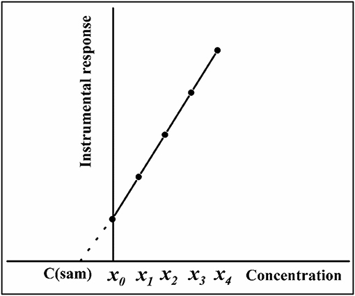
Figure 1. SA calibration plot using four addition points (x1-x4). Extrapolation is represented by a broken line, and x0 is the sample with no standard addition.
Several papers have applied the extrapolation strategy for SA, but according to Andrade et al. (2013), the use of interpolation increases accuracy and precision because the central part of the regression line (where the confidence interval of the regression is narrow) is used in the calculations. Additional details on the mathematical description and theory of the SA method can be found in the literature in works by Kolthoff and Lingane (1939), Bader (1980), Currie (1998), Bergfeld et al. (2005), Brown et al. (2007, 2011, 2017), Brown (2009), Kelly et al. (2011), Brown and Gillam (2012a,b), Brown and Mustoe (2014), Gonçalves et al. (2016a), Andersen (2017), among others.
There are several strategies to perform SA. In voltammetric analysis, frequently only two calibration points are used, with solution 1 containing the sample with no standard added, and solution 2 consisting of the sample with standard addition (Kolthoff and Lingane, 1939; Kelly et al., 2011). In these cases, a mathematical equation, rather than graphical extrapolation, has been used to determine the analyte concentration in the sample. In spectrometric analysis, typically five or six calibration points and graphical extrapolation have been used, since the 1950s, for calculating the analyte concentration in the sample (Kelly et al., 2011).
Bader (1980) described a systematic approach to SA including five different strategies to perform this calibration method when analyte concentration and instrument response present a linear relationship. As discussed by the author, a different mathematical equation is used to calculate the unknown analyte concentration in the sample for each of the five proposed strategies. The mathematical equations use values for the intercept, slope, the concentration of the standard solution, and the volumes of both standard solution and sample. Kelly et al. (2008) revised the equations for all five SA strategies proposed by Bader considering a gravimetric approach. Masses rather than volumes were used in this case, and according to the authors, such approach makes the SA method suitable not only for liquid solutions, but also for solid samples.
When several solutions containing the same amount of sample and different amounts of standard solution are prepared separately, SA is known as conventional standard additions calibration (C-SAC). The first of these solutions contains only the sample, while increasing concentrations of the analyte are added the other solutions (Figure 1). In sequential standard additions calibration (S-SAC), different amounts of standard are added to a single flask containing the sample. In S-SAC, the original sample in a container is analyzed and the instrument response is recorded (Brown et al., 2007). Then, a certain amount of standard solution is added to the same container and the analytical signal is recorded once again. The procedure is repeated, with additional volumes of the standard solution sequentially added to the same container and the analytical signals recorded in each case. The SA calibration plot is then built with analyte concentrations (or standard volumes) added to the sample (x-axis) vs. instrument response (y-axis). Another application for S-SAC was proposed by Brown et al. (2017), in which the final volume of the mixture is used to determine the concentration of relevant impurities in a blank matrix of gas. The constant final volume strategy is only applicable to gas samples, but the extrapolation method used with it is the same as the one used with variable-final-volume S-SAC.
Brown (2009, 2011), Brown and Gillam (2012a,b) and Brown et al. (2007, 2011) evaluated the differences between C-SAC and S-SAC regarding precision, use of extrapolation or interpolation, and homoscedasticity or heteroscedasticity. The authors have shown that S-SAC can replace C-SAC if an adequate quantity of standard solution is added to the sample, and if the appropriated equation (which was proposed by the authors) is used to determine the analyte concentration in the sample. The main advantages of S-SAC when compared to C-SAC is its simplicity, lower costs, higher sample throughput, and generation of less residues (Brown et al., 2007; Brown, 2009, 2011). However, the application of S-SAC may be limited to non-destructive instrumental methods, such as voltammetry and UV-visible spectrophotometry. So far, there is no report in the literature of the use of S-SAC in spectrometric instrumental methods. However, it may be easily applied if the volume of sample consumed during the analysis is small, and the volume of standard solution added in each step is negligible in comparison with the total volume of the sample solution. For example, 10.0 μL of standard solution is added to 25.0 mL of sample in each standard addition step in a GF AAS or a tungsten coil atomic emission spectrometry (WCAES) determination (which typically consume 10–25 μL of sample per run). In this case, because the volumes of standard solution added and solution mixture consumed during the analysis have no significant effect on the final solution volume, S-SAC can be successfully applied. It is important to note, though, that S-SAC is an irreversible method, i.e., once the standard solution is added, there is no way to re-run a sample to check a previously recorded signal.
Other approaches to SA include, for example, the bracket standard additions method described by Abbyad et al. (2001) to improve precision in ICP-MS. It consists of recording the analytical signal before and after adding the standard solution to the sample, and using the mean of the two measurements in specific equations to compensate for instrument drift. The authors also evaluated different levels of standard addition and showed that similar precisions are obtained when the analyte concentration in the standard solution is the same as, or 7- to 50-fold higher than that of the sample. In another work, Boto and Murphy (2005) proposed modifications to the SA equation to overcome issues associated with its application to samples containing very high concentrations of analyte. Their method was used in XRF and may be applied to other instrumental analytical techniques.
Before the revision of Bader's equations by Kelly et al. (2008), Christopher et al. (2005) had introduced the gravimetric approach to the SA method. In addition to its compatibility to solid samples as discussed earlier, the authors pointed out that the gravimetric approach may also improve accuracy when compared to the volumetric approach. Internal standardization was combined with the gravimetric approach to overcome the inconvenience associated with sample solution dilution when the standard is added. The IS species and the analyte standard were gravimetrically added to each flask containing the sample (usually a certified reference material), with concentrations varying from none to a high addition level. According to the authors, the main advantage of this approach is that quantitative adjustment of volume is not necessary, as the IS can correct for dilution effects. Furthermore, if samples are homogenous and have identical matrix, it is not necessary to build a calibration curve for each sample, and the analyte concentration can be determined from the slope of a curve built with the certified reference material. In this case, the calibration plot contains the mass of analyte added per gram of sample on the x-axis, and the analyte/IS signal ratio, multiplied by mass of IS per gram of sample, on the y-axis.
Zhu and Chiba (2012) proposed combining the SA gravimetric approach with internal standardization using a single standard addition point for elemental analysis by ICP-MS. The analyte concentration in the sample is determined by using the appropriate equation and considering the signal and mass of analyte and IS in both the standard solutions and the sample. A different mathematical equation is proposed if the mass of the IS species is not known. As reported by the authors, any element can be used as IS. However, because there is no requirement for similar physicochemical properties nor close m/z values for analyte and IS, the element selected as an IS must present a high signal intensity, stable concentration, and have no signal overlap with the analyte. This strategy was also used by Gao et al. (2015a,b) to determine As and Sb in seawater and natural water by ICP-MS. As one would expect, the one-point standard addition calibration method is simpler, less expensive and faster than the traditional multi-level standard additions (Andrade et al., 2013). However, similar to EC, the more calibration points used, the more precise and accurate the results (Miller and Miller, 1984). Table 3 shows some selected applications using the SA method applied to instrumental spectrometric techniques, including the combination of SA and IS, which is frequently used in LIBS.
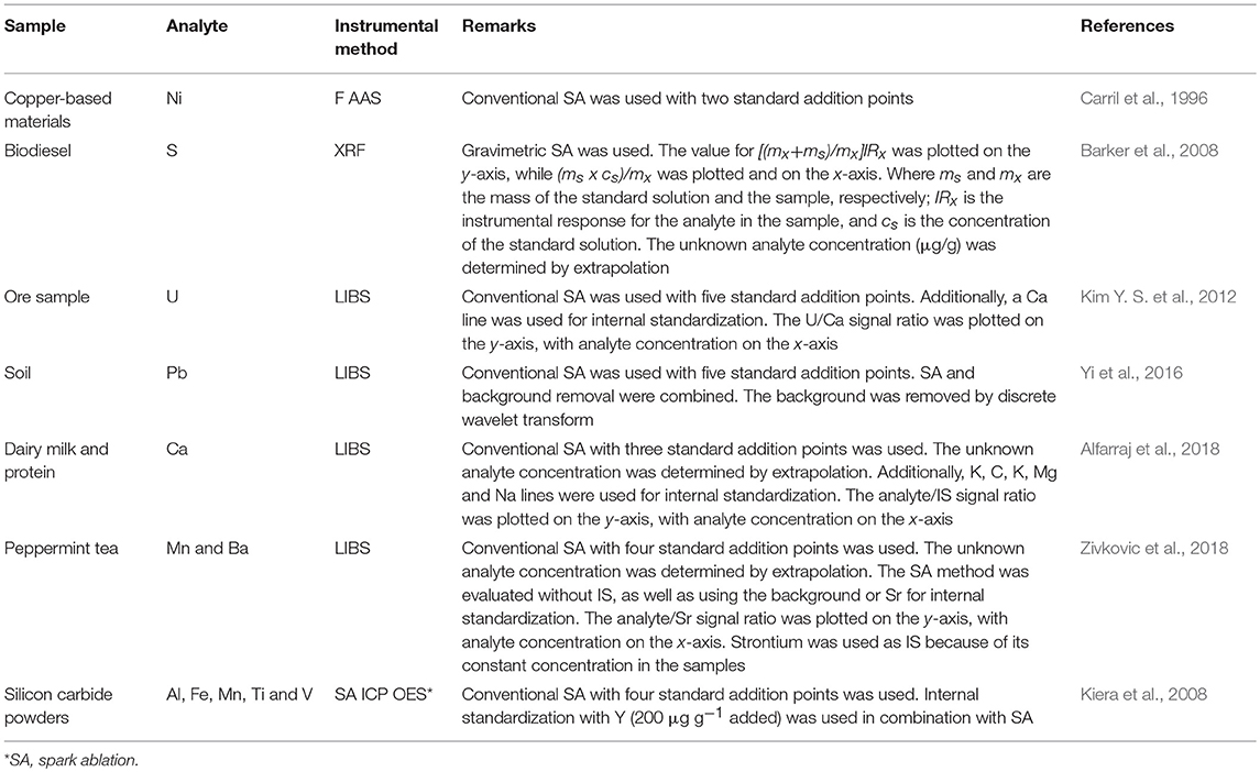
Table 3. Selected applications of the SA method associated with instrumental spectroanalytical techniques.
The main advantage associated with the SA method is that the sample itself is used to prepare the calibration solutions, consequently matrix effects are corrected and no previous knowledge of the sample matrix is required (Kelly et al., 2011). The SA method has been shown efficient at correcting for rotational effects, which involve non-analyte constituents of the sample and their impact on the calibration curve slope. On the other hand, the SA method is not suitable for correcting for translational effects, which are related to the background signal and only affect the calibration curve intercept (Thompson, 2009; Andrade et al., 2013; Andersen, 2017). In this case, concomitant substances in the matrix cause systematic variation of the analytical signal, compromising accuracy and precision (Thompson, 2009; Andrade et al., 2013). The main drawback associated with the SA method is the requirement for building a calibration curve for each sample. This issue becomes especially critical when a large amount of samples has to be analyzed, as SA's sample throughput is considerably lower than EC, MMC, and IS. Additionally, the SA method may become ineffective, due to large experimental error, when the chemical form of the analyte is different in the sample and standard solution added, when the analyte is present at very high concentrations in the sample, and depending on the ratio between the concentration of analyte in the standard solution added and in the sample (Boto and Murphy, 2005; Andrade et al., 2013).
Non-traditional Calibration Methods Applied to ICP-MS
Several non-instrumental strategies have been described to minimize spectral and non-spectral interferences in ICP-MS determinations. Mathematical correction equations are an example of a data-processing approach used prior to calibration to minimize spectral interferences. By knowing the natural abundance of each isotope of an interfering element and recording its signal intensity at an alternative m/z, one can easily subtract the interfering signal at the analyte's m/z (Goossens et al., 1994; Neubauer, 2010; Thomas, 2013). Although efficient in some specific cases involving isobaric monoatomic interfering species, mathematical correction equations present several drawbacks. They perform poorly when high concentrations of the interfering species are present. On the other hand, if there is no interference, applying a correction equation will cause overcorrection, which in many cases results in obviously wrong negative analyte concentrations. In addition, increasingly more complex equations are required if the alternative isotope used for signal correction suffers itself from spectral interferences.
As an example of a strategy to minimize non-spectral interferences in ICP-MS, naturally-occurring polyatomic ions such as ArH+, , ArO+, and have been employed as internal standard species to correct for matrix effects and signal drift (Beauchemin et al., 1987). These ions were used, for example, to minimize signal bias in As, Co, Mg and Mn determinations, and the species was applied to correct for transport and matrix effects in the direct analysis of solids by ETV-ICP-MS (Grégoire et al., 1994; Chen and Houk, 1995; Vanhecke et al., 1995).
More recently, four non-conventional calibration strategies have been reported to improve accuracy in quadrupole-based ICP-MS analyses. The IFS method is similar to the previously discussed strategy of using naturally-occurring polyatomic ions to correct for signal bias. However, it is used to minimize spectral interferences, and therefore, works differently from a traditional IS method. The other three strategies, SDA, MICal, and MSC, are used to minimize non-spectral interferences, and are based on a matrix-matching approach which uses only two calibration solutions per sample. These novel strategies will be discussed in detail in the following sections.
Theory and Mathematical Description of Some Non-traditional Calibration Methods
The Interference Standard Method (IFS)
The IFS method is a calibration strategy proposed to overcome polyatomic interferences in ICP-QMS. It relies on the hypothesis that interfering ions and naturally-occurring IFS species such as 36Ar+, 36ArH+, and 38Ar+ present similar behaviors in the plasma (Donati et al., 2011). Additional evidence of this principle has been provided in a recent work using high-resolution sector field ICP-MS measurements (Amais et al., 2014). Different from a conventional internal standardization method, the IFS strategy considers correcting variations in the interfering signal rather than in the analytical signal. Therefore, signal bias caused by ions and polyatomic species naturally occurring in the plasma, or formed by interactions between these and the sample solution, can be minimized by using the signal ratio between analyte and IFS species during calibration (Donati et al., 2011). It is important to note that the relatively low resolution of an ICP-QMS is not enough to separate analyte and interfering signals, so both are divided by the IFS signal during data processing. The main premise of the IFS method is that because interfering polyatomic species and IFS species behave similarly, their signal ratio will be relatively constant, which can then minimize biases caused on the analytical signal by variations in the unresolved isobaric interfering signal. Thus, a typical IFS calibration plot has the ratio of unresolved analyte + interfering signal/IFS signal on the y-axis (dependent variable), and analyte concentration on the x-axis (independent variable). Compare, for example, Figures 2 and 3, which represent the calibration plots for Si determination by ICP-QMS with and without applying the IFS method. Using the regression equation in Figure 2 to calculate the analyte concentration in a sample spiked with 10.0 μg/L of Si results in a negative value: −10.7 ± 1.5 μg/L (n = 3). On the other hand, the regression equation based on the IFS method (Figure 3) provides an accurate result of 9.8 ± 1.5 μg/L of Si (n = 3). This example highlights how severe the effect from the 14 ion can be on Si determination, at the m/z 28, when no signal correction nor other interference elimination strategy is used in ICP-QMS. It also shows the efficiency of the IFS method at minimizing spectral interferences and improving accuracy. As demonstrated in previous works (Donati et al., 2011, 2012a; Amais et al., 2014), the 38Ar+ IFS ion has a similar behavior to the 28 ion, and when their signal ratio is used for calibration, the interfering effect is significantly reduced.
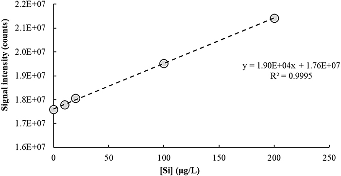
Figure 2. Calibration plot used to determine Si in a 1% v/v HNO3 matrix by ICP-QMS (m/z = 28). No collision/reaction gas was used.
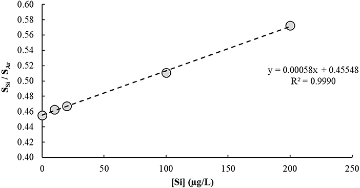
Figure 3. Calibration plot used to determine Si in a 1% v/v HNO3 matrix by ICP-QMS (m/z = 28) using the IFS method. The 38Ar+ ion was used as IFS species, and the analyte-to-IFS signal ratio was plotted on the y-axis. No collision/reaction gas was used.
These results can be further understood by analyzing Equations (1) and (2), where R is the calculated analyte recovery (%), SI is the interfering ion signal collected during calibration, VI is percent difference between interfering ion signal values recorded for the sample and its corresponding standard solution (i.e., it represents how much the interfering ion signal has varied from the time the calibration standards were run to when the sample was analyzed), SA is the analytical signal, and VIFS is the percent difference between IFS signal values recorded for the sample and its corresponding standard solution (i.e., similar to VI).
From Equation (1), one can infer that the larger the variation in the interfering ion signal (VI) and the larger the SI/SA ratio, the worse the analyte recoveries (Donati et al., 2011; Amais et al., 2014). In the example of Si determination discussed earlier, VI might have been negative, i.e., the interfering ion signal was lower when the sample was analyzed than when its corresponding standard solution was run, which resulted in a negative R (%). Considering that N2 gas is the major component of air, and it is dragged into the Ar plasma during ICP operation, it is also reasonable to assume the 14 signal (SI) was significantly higher than the 28Si+ signal (SA) during the analysis, which also contributed to the poor recovery. Alternatively, when the IFS method was applied, it is reasonable to assume that VI and VIFS were relatively similar (Equation 2), which reduced the impact of the large SI/SA ratio on analyte recovery (i.e., SI/SA is multiplied by a number close to zero), and provided a more accurate concentration value. Similar results and related discussions were presented in a recent work employing high-resolution ICP-MS measurements, which also described the fundamentals of the IFS method in more detail (Amais et al., 2014).
Standard Dilution Analysis (SDA)
SDA is a calibration method that may be applied to any instrumental technique which accepts liquid samples and is capable of monitoring multiple analytical signals either simultaneously or fast sequentially (Jones et al., 2015; Gonçalves et al., 2016b; Virgilio et al., 2016a,b). It is an example of analytical strategy to minimize non-spectral interferences, as it combines the traditional methods of IS and SA. Thus, SDA is able to simultaneously correct for matrix effects and signal fluctuations due to changes in sample size, orientation, or instrumental parameters (Jones et al., 2015).
Applying the SDA method involves the continuous monitoring of both analytes and an internal standard species, as two calibration solutions (S1 and S2) are mixed in a single container. These solutions contain the same amount of sample, so no matrix effect is expected. S1 has a 1:1 proportion of sample and a standard solution containing the analytes and the internal standard (IS), while S2 has the same 1:1 mixture of sample and blank. Data is initially collected, in a time-resolved manner, as S1 is introduced into the ICP-MS. When S2 is poured into the same container with S1, the sample matrix concentration is not affected (because both S1 and S2 contain the same amount of sample), but the standards and the IS are gradually diluted as the two solutions mix (hence SDA). Both analytical and IS signals slowly drop as a result, creating a negative slope on the signal intensity vs. time plot. In the negative slope region, known as the SDA region (Figure 4), each point represents a different concentration of analyte and IS. Thus, similarly to a conventional EC plot, these “calibration points” can be used to determine the analyte concentration in the sample. Only in this case, several calibration points are potentially available, as signals are collected typically every second (Virgilio et al., 2016a).
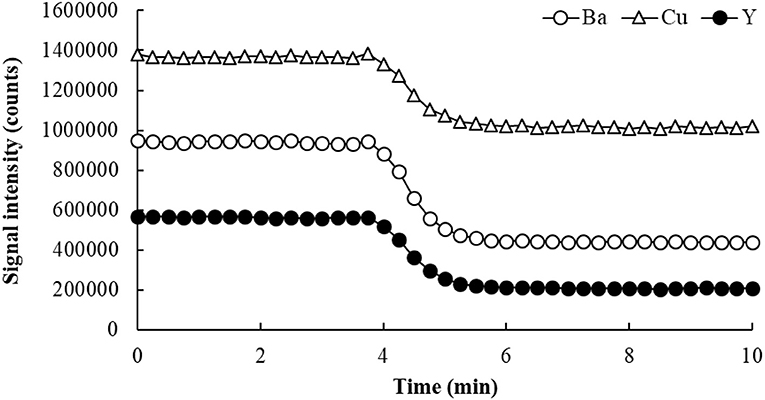
Figure 4. SDA plot for the determination of Ba and Cu in Oyster Tissue (NIST 1566b) by ICP-MS. Yttrium was used as internal standard, and He flowing at 3.5 mL/min was used in the collision/reaction cell.
The SDA calibration curve is built by plotting the analyte-to-IS signal ratio (SA/SIS) on the y-axis, and the reciprocal of the IS concentration (1/CIS) on the x-axis (Jones et al., 2015; Virgilio et al., 2016b). Figures 4 and 5 show an example of SDA application to determine Ba and Cu in a standard reference material of Oyster Tissue (NIST 1566b). Values for CIS are calculated from the known IS concentration added to S1. In this case, any point on the plateau preceding the negative slope in Figure 4 corresponds to that concentration (50 μg/L in this example), and each subsequent point in the SDA region has a proportionally lower concentration. According to Equation (3) (Jones et al., 2015; Gonçalves et al., 2016b; Virgilio et al., 2016a,b), the analyte concentration in the sample (C(sam)A) can be found from the slope and intercept of the SDA calibration plot, which are represented in Equations (4–6).
Where mA and mIS are calibration curve sensitivities for analyte and internal standard, respectively, and C(std)A is the concentration of analyte in the standard solution.
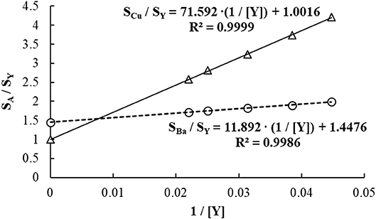
Figure 5. Calibration plots created from the SDA region (negative slopes) in Figure 4. The concentrations of Ba, Cu, and Y added to S1 were 50 μg/L each.
Because both C(std)A and CIS are known and constant (as they were added to S1), C(sam)A is readily calculated from the SDA calibration curve equation using Equation (6). Considering that C(std)A = CIS = 50 μg/L in the example shown in Figures 4 and 5, the concentrations of Ba and Cu in solution are 8.22 and 71.5 μg/L, respectively. These values correspond to 8.22 and 71.5 mg/kg in the sample replicate analyzed (0.2499 g of sample digested, with solution volume made up to 25.0 mL and then diluted 10-fold before analysis), and recoveries of 95.6 and 99.9%, respectively.
Multi-Isotope Calibration (MICal) and Multispecies Calibration (MSC)
Both MICal and MSC are based on a dimension rarely explored in calibration, which is related to the capability of modern instruments to simultaneously, or at least fast-sequentially, monitor several analytical signals. Different from a traditional calibration method, which is based on determining a mathematical function relating analyte concentration and instrument response at a specific region of the spectrum, MICal and MSC use the instrument response from a single analyte concentration recorded at multiple points of the spectrum for calibration. Although applied for ICP-MS analysis, both MICal and MSC are an extension of the multi-energy calibration method (MEC), which has been recently applied in ICP OES, MIP OES and HR-CS F AAS (Virgilio et al., 2017). As with SDA, MEC, MICal and MSC rely on a matrix-matching strategy to minimize matrix effects. Calibration solutions are prepared in the same fashion as S1 and S2 in SDA, except they are run separately in MEC, MICal and MSC and no internal standard is required. The calibration plot is built with signals recorded for S1 and S2 on the x-axis and y-axis, respectively. Each point in the calibration plot corresponds to a different wavelength (MEC; Virgilio et al., 2017), isotope (MICal; Virgilio et al., 2018), or molecular ion (MSC; Williams and Donati, 2018) of the same analyte; all produced from a single analyte concentration, which was added to S1.
Because MEC, MICal and MSC rely on the same principle, they can be mathematically described using the same equations. Consider the following functional relationships for S1 and S2 (Equations 7 and 8, respectively), where S(Xi)Sam+Std and S(Xi)Sam are the instrument responses for a given (Xi) analytical signal source (i.e., wavelength, isotope or molecular ion); m is a proportionality constant; and C(A)Sam and C(A)Std are the analyte concentrations in the sample and in the standard solution added to S1.
Given the same set of instrumental conditions and the same matrix composition since both S1 and S2 contain the same amount of sample, m will have the same value in both Equations (7) and (8), which may then be combined (Equation 9), and rearranged to give Equation (10).
By plotting S(Xi)Sam+Std (from S1) on the x-axis, and S(Xi)Sam (from S2) on the y-axis, with multiple signal sources of the same analyte (Xi, Xj, Xk, …, Xn) corresponding to different points on the calibration graph, the slope of the linear regression model will be:
and because C(A)Std is known, the analyte concentration in the sample may be easily determined by rearranging Equation (11), which leads to Equation (12).
A typical MICal calibration plot is depicted in Figure 6. In this example, a tap water sample spiked with 10 μg/L of Cd is analyzed by ICP-MS. By applying Equation (12) and considering a [C(A)Std] of 30 μg/L, the concentration of Cd in the sample is calculated as 10.3 μg/L, i.e., a recovery of 103%.
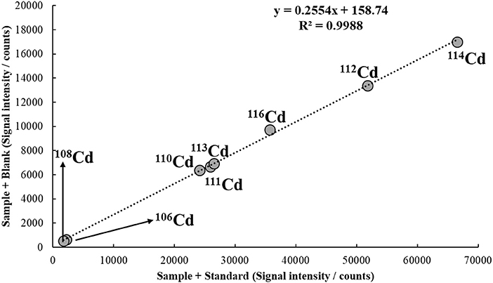
Figure 6. MICal plot used to determine Cd in a tap water sample spiked with 10 μg/L of the analyte. The concentration of Cd standard added to S1 [C(A)Std] was 30 μg/L. He flowing at 3.5 mL/min was used in the collision/reaction cell.
For simplicity, a 1:1 mixture of sample and standard solution (S1), and sample and blank (S2) is frequently used in MEC, MICal and MSC. However, any other proportion may be used, as long as both S1 and S2 contain the same amount of sample. A 20% sample/80% standard solution (or blank) may be adopted, for example, to further minimize matrix effects; or a 70% sample/30% standard solution (or blank) may be used to improve sensitivity. In such cases, however, a dilution factor must be included in Equation (12), as shown in Equation (13), where VStd corresponds to the volume of standard solution added to S1, and Vsam is the volume of sample added to both S1 and S2 (Virgilio et al., 2018).
As an example of application using Equation (13), Figure 7 shows the MICal plot to determine Cd in tap water similar to the one discussed in Figure 6. In this case, however, S1 and S2 were prepared with 70% sample and 30% of standard solution or blank. Considering the same C(A)Std, i.e., 30 μg/L, the concentration of Cd in solution calculated from Equation (13) is 9.44 μg/L, which corresponds to a 94% recovery from the spiked value of 10 μg/L. Note that if VStd = VSam, i.e., a 1:1 mixture is used in S1 and S2, Equation (13) simplifies to Equation (12).
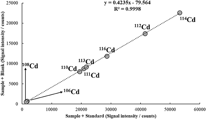
Figure 7. MICal plot used to determine Cd in a tap water sample spiked with 10 μg/L of the analyte. S1 and S2 were prepared with 70% of sample and 30% of standard solution or blank. The concentration of Cd standard added to S1 [C(A)Std] was 30 μg/L. He flowing at 3.5 mL/min was used in the collision/reaction cell.
Applications, Advantages, and Potential Limitations of IFS, SDA, MICal and MSC
Tables 4 and 5 list recent applications, and the advantages and potential limitations of each of the non-traditional calibration methods discussed here. Of the four strategies discussed, IFS and SDA are the more mature methods, whereas MICal and MSC have been recently published in the literature as proofs-of-concept. The IFS method is the only non-matrix-matching approach, but it is also the only one capable of minimizing spectral interferences. It requires no instrumental modification beyond simple ICP-QMS, nor the addition of an internal standard to the sample matrix. Since its original description in the literature in 2011, the IFS method has been successfully applied to the determination of several analytes in different sample matrices (Amais et al., 2011, 2012, 2014; Donati et al., 2011, 2012a,b; Amaral et al., 2013; Latorre et al., 2015; Table 4). Although the magnitude of the IFS signal has no effect on accuracy, its fluctuation during the analysis (VIFS) may negatively impact analyte recoveries (first part of Equation 2; Amais et al., 2014). Such effect is due to the low resolution of the ICP-QMS, i.e., the IFS signal divides the unresolved analyte plus interfering ion signal. Therefore, a large VIFS value (e.g., 30%) will result in poor recoveries (e.g., 76.9%) even if VIFS = VI, according to Equation (2). Fortunately, this is rarely the case in modern ICP-MS instruments and for the relatively high IFS signals (low RSDs) used for calibration.
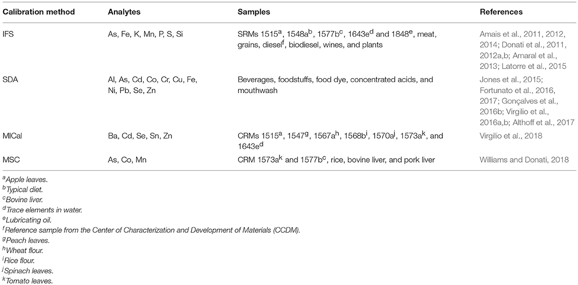
Table 4. Applications of the non-traditional calibration methods and listed references.
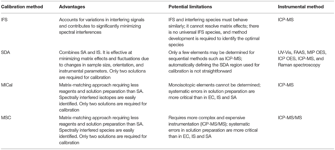
Table 5. Advantages and potential limitations of IFS, SDA, MICal and MSC, and the instrumental methods in which they have been used.
On the other hand, the efficiency of the IFS method is directly related to how well VIFS matches the signal fluctuation of the interfering species (VI) (Donati et al., 2011; Amais et al., 2014). If VIFS is similar to VI, accurate results will be achieved even if the interfering signal is significantly higher than the analytical signal (note that there is no requirement for the intensities of interfering and IFS species, SI and SIFS, to match according to Equation 2). For example, if VI and VIFS are 5 and 4.9%, respectively, and SI/SA = 10, the analyte recovery will be 96.3% (Equation 2). Using the same example, if VI = 5% and VIFS = 1%, the analyte recovery will be 138.6%. Alternatively, if VI = VIFS = 5%, the analyte recovery will be 95.2% even if SI/SA = 106. Therefore, in order to obtain optimal results using the IFS method, (VI–VIFS) must be small if II/IA is large; or II/IAmust be small if (VI–VIFS) is large. However, potential consequences of these limitations are easily identified by the analyst, who can choose the most appropriate IFS species based on results from method development experiments. The entire procedure is usually easy since both analytical and IFS signals are monitored during analysis and one can decide whether to use the analyte/IFS signal ratio for calibration after the run.
SDA, MICal and MSC are calibration strategies used to minimize matrix effects rather than to correct for spectral interferences. Therefore, different from IFS, an additional procedure to eliminate spectral interferences is commonly required when employing these methods (e.g., He has been used as collision gas in the examples shown in Figures 4–7). SDA, MICal and MSC are relatively easy to implement, and require less reagents and allow for higher sample throughputs when compared to the traditional SA method. Because the same amount of sample is present in the calibration solutions, matrix effects are not of concern. Thus, SDA, MICal and MSC accuracies are comparable and often better than the traditional EC, IS, and SA methods (Jones et al., 2015; Virgilio et al., 2018; Williams and Donati, 2018). SDA may be more broadly applicable than MICal and MSC, as it has been successfully used in UV-vis, FAAS, MIP OES, ICP OES, and Raman spectroscopy in addition to ICP-MS (Jones et al., 2015; Fortunato et al., 2016, 2017; Gonçalves et al., 2016b; Virgilio et al., 2016a,b; Althoff et al., 2017; Table 4). Because it employs an internal standard, it is also capable of correcting for signal fluctuations due to instrument variations. However, its gradient dilution nature is a limiting factor in applications involving sequentially collected data such as in ICP-MS and MIP OES (Gonçalves et al., 2016b; Virgilio et al., 2016a; Althoff et al., 2017). With a fast dilution process (when S1 and S2 are mixed in the same container), the larger the number of analytes the fewer the points available for calibration in the negative slope region of the SDA plot (Figure 4). Therefore, different from a simultaneous SDA-ICP OES measurement, in which many calibration points are available, ICP-MS determinations are limited to a few SDA points (Figure 5). This limitation may be overcome by using an ICP-(TOF)MS, for example. Another minor difficulty encountered in SDA applications is associated with data processing. Establishing a fast, systematic procedure to automatically define the SDA region and use its data points for calibration is less than straightforward. However, computer algorithms and hardware automation may be easily implemented, which can significantly streamline the entire SDA process. An instrument setup including, for example, an automatic sampler with seamless solution mixing, and data processing software to select the SDA region and automatically calculate the analyte concentration in the sample may contribute to a more broad adoption of SDA. This is a critical need to allow for SDA and other strategies discussed here to be effectively used in routine analysis.
A significant amount of effort has been placed toward resolving spectral interferences in ICP-QMS determinations, with collision/reaction cells (CRCs) and ICP-MS/MS representing the current state of the art (Tanner et al., 2002; Koppenaal et al., 2004; Bolea-Fernandez et al., 2015, 2017; Lum and Sze-Yin Leung, 2016). Despite these efforts, ICP-MS is still susceptible to relatively intense matrix effects, which may be caused by space charge effects, or stem from samples containing organic solvents or high concentrations of acids, carbon species, and easily ionizable elements (Gajek and Choe, 2015; García-Poyo et al., 2015; Leclercq et al., 2015). Although SDA and the traditional SA method are both efficient at minimizing matrix effects, the former is limited by the sequentially recorded ICP-MS data and the restrictions on the number of analytes determined in each run (Virgilio et al., 2016a), and the latter is time and reagent consuming. On the other hand, MICal and MSC have been specifically developed for ICP-MS applications (Table 4). They are more easily implemented than SDA, as no fast dilution process is required, and common automatic sampler devices can be used for calibration. An additional advantage of using these methods when compared with SDA and the traditional EC, IS, and SA is that spectral interferences may be easily identified as an outlier point on the linear region of the calibration curve (Virgilio et al., 2017, 2018; Williams and Donati, 2018). On the other hand, systematic errors during solution preparation are not as easily detected as in the traditional methods. Thus, additional caution must be taken when preparing the standard solution added to S1 to prevent any systematic bias. Some other limitations include MICal's requirement for analytes presenting at least two stable and sensitive isotopes, and MSC's application only to instruments with MS/MS capabilities (Virgilio et al., 2018; Williams and Donati, 2018). Therefore, MICal is not applicable to monoisotopic analytes such as As, Mn and P. In a sense, MSC complements MICal, as molecular ions of monoisotopic analytes formed in the CRC of an ICP-MS/MS instrument are used for calibration. In the recently published proof-of-concept work by Williams and Donati (2018), signals from oxide and ammonia cluster ions of As, Co and Mn are used as calibration points in the MSC graph. However, in principle, any ion containing the analyte can be used in MSC. The method was successfully used to analyze CRMs of tomato leaves and bovine liver, with accuracies comparable to and often better than EC, IS, and SA. Commercial samples of rice and liver were also analyzed to demonstrate the applicability of the method in routine analyses.
Boundaries of Application for MICal and MSC
SDA is similar to the traditional calibration methods regarding its application boundaries, i.e., it may be effectively used within the linear dynamic range of a given analyte at a certain wavelength (or for a certain isotope). On the other hand, neither MICal nor MSC follow this precept, as both are based on analytical signals from multiple sources and with different sensitivities. By comparing Figures 6 and 7, it can be seen that the higher the analyte concentration in the sample [C(A)Sam] the larger the MICal (or MSC) slope. From Equation (11), one can observe that as C(A)Sam becomes significantly higher than the analyte concentration in the standard added to S1 [C(A)Std], the slope approaches a value of 1. In this case, C(A)Std becomes negligible as compared with C(A)Sam, which can compromise the accuracy of the method (Virgilio et al., 2018; Williams and Donati, 2018). Alternatively, if C(A)Sam is significantly lower than C(A)Std, accuracy will also be compromised, as the slope will approach zero. Therefore, both MICal and MSC will perform at their best when the calibration curve slopes are away from extreme values (i.e., away from 0 and 1; Virgilio et al., 2018; Williams and Donati, 2018).
One can establish the application boundaries (or working ranges) for MICal and MSC based on expected or ideal calibration curve slopes. It is possible then to determine the minimum C(A)Std and C(A)Sam values that will ensure the desired slope range. Consider, for example, a working range with slopes between 0.1 and 0.9. By plugging these values into Equation (12), the lower and higher boundaries will correspond to the relationships shown in Equations (14) and (15), respectively.
An additional restriction in applying the MICal and MSC methods relates to the limits of quantification (LOQ). The minimum value for C(A)Sam must be ≥ LOQ. Thus, replacing C(A)Sam with LOQ in Equation (14) gives Equation (16):
Therefore, C(A)Std ≥ 9 LOQ and C(A)Sam ≥ LOQ will ensure a minimum slope of 0.1. The higher application boundary can then be defined by combining Equations (15) and (16): C(A)Sam = 81 LOQ. Thus, if C(A)Std = 9 LOQ, analyte concentrations in the sample between 1 LOQ and 81 LOQ can be effectively determined, as 0.1 ≤ slope ≤ 0.9. Experimentally, the sample can be diluted, or the standard solution concentration can be adjusted to ensure these values. A practical strategy for doing that is to compare the analytical signal intensities from a given source (i.e., isotope or complex ion containing the analyte) for sample and standard solution. Considering that analytical signal intensity [S(A)] and analyte concentration [C(A)] are proportional, Equations (14) and (15) can be rewritten as S(A)Sam/S(A)Std = 0.111, and S(A)Sam/S(A)Std = 9. Thus, one can run the sample and the standard solution separately and compare their analytical signal intensities for the most sensitive isotope or the most sensitive analyte ion complex. If their signal ratio is between 0.111 and 9, the calibration curve slope should be approximately in the 0.1–0.9 range. It is important to note that this measurement is only approximate because sensitivity differences are expected between sample and standard solution due to matrix effects. However, it allows for a fast semi-quantitative assessment of the analyte concentration in the sample and contributes to the decision of whether concentration adjustments are necessary.
Conclusions
The ideal calibration method is cost-effective, simple, widely applicable, and capable of correcting for spectral and non-spectral interferences, which results in significant improvements in precision, accuracy and sample throughput. However, as in many other contexts, there is no such thing as a one-size-fits-all calibration method. Different strategies, or a combination of methods may be used with complex-matrix samples, and instrumental or sample preparation strategies may be required when severe interfering effects are present.
We hope this review paper has demonstrated that calibration is essential to any analytical procedure, and the analyst always needs to consider its effects on accuracy, precision and sample throughput when determining the most appropriate method for a given application. As discussed here, a carefully chosen calibration method can improve the analytical performance of an instrumental spectrochemical technique. It may be a simple, fast and cost-effective alternative to instrumental solutions dealing with spectral and non-spectral interferences. A summary of the most adequate general applications for each of the calibration methods discussed in this work is shown in Figure 8. As analytical instrumentation evolves, new calibration approaches based on innovative data processing strategies should be developed to support faster and more accurate procedures, which will ultimately contribute to a better understanding of the role of trace elements in chemical processes, human health and the environment.
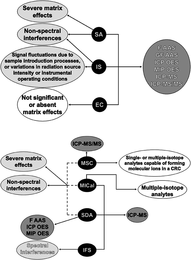
Figure 8. Summary of the most adequate general applications for EC, IS, SA, IFS, SDA, MICal, and MSC.
Author Contributions
JC and AB performed the general literature review. AB and JN prepared the traditional calibration methods section. JC and GD prepared the non-traditional calibration methods section. JN and GD edited the manuscript.
Conflict of Interest Statement
The authors declare that the research was conducted in the absence of any commercial or financial relationships that could be construed as a potential conflict of interest.
Acknowledgments
The authors are grateful to the Conselho Nacional de Desenvolvimento Científico e Tecnológico and the São Paulo Research Foundation (CNPq, Instituto Nacional de Ciências e Tecnologias Analíticas Avançadas, Grant No. 573894/2008-6, and FAPESP Grant No. 2014/50951-4) for the financial support. This study was also financed in part by the Coordenação de Aperfeiçoamento de Pessoal de Nível Superior – Brasil (CAPES) – Finance Code 001. JN is also thankful to the CNPq (Grant No. 303107/2013-8) for the fellowship. Support from the National Science Foundation's Major Research Instrumentation Program (NSF MRI, grant CHE-1531698), and the Department of Chemistry and Graduate School of Arts and Sciences at Wake Forest University are also greatly appreciated.
References
Abbyad, P., Tromp, J., Lam, J., and Salin, E. (2001). Optimization of the technique of standard additions for inductively coupled plasma mass spectrometry. J. Anal. Atomic Spectrom. 16, 464–469. doi: 10.1039/b100672j
ABNT NBR 15556 (2008). Fat Oil and Derivatives. Fatty Acid Methyl Esters. Determination of the Sodium, Potassium, Calcium and Magnesium Contents by Atomic Absorption Spectrometry. São Paulo.
Aguirre, M. Á., Kovachev, N., Almagro, B., Hidalgo, M., and Canals, A. (2010). Compensation for matrix effects on ICP-OES by on-line calibration methods using a new multi-nebulizer based on Flow Blurring® technology. J. Anal. Atomic Spectrom. 25:1724. doi: 10.1039/c004854b
Alfarraj, B. A., Sanghapi, H. K., Bhatt, C. R., Yueh, F. Y., and Singh, J. P. (2018). Qualitative analysis of dairy and powder milk using laser-induced breakdown spectroscopy (LIBS). Appl. Spectrosc. 72, 89–101. doi: 10.1177/0003702817733264
Almeida, J. S., Brand, C., and Santos, G. L. (2016). Fast sequential determination of manganese and chromium in vegetable oil and biodiesel samples by high-resolution continuum source graphite. Anal. Methods 8, 3249–3254. doi: 10.1039/c6ay00165c
Althoff, A. G., Williams, C. B., McSweeney, T., Gonçalves, D. A., and Donati, G. L. (2017). Microwave-induced plasma optical emission spectrometry (MIP OES) and standard dilution analysis to determine trace elements in pharmaceutical samples. Appl. Spectrosc. 71, 2692–2698. doi: 10.1177/0003702817721750
Amais, R. S., Donati, G. L., and Nóbrega, J. A. (2011). Application of the interference standard method for the determination of sulfur, manganese and iron in foods by inductively coupled plasma mass spectrometry. Anal. Chim. Acta 706, 223–228. doi: 10.1016/j.aca.2011.08.041
Amais, R. S., Donati, G. L., and Nóbrega, J. A. (2012). Interference standard applied to sulfur determination in biodiesel microemulsions by ICP-QMS. J. Braz. Chem. Soc. 23, 797–803. doi: 10.1590/S0103-50532012000500002
Amais, R. S., Donati, G. L., Schiavo, D., and Nóbrega, J. A. (2013). A simple dilute-and-shoot procedure for Si determination in diesel and biodiesel by microwave-induced plasma optical emission spectrometry. Microchem. J. 106, 318–322. doi: 10.1016/j.microc.2012.09.001
Amais, R. S., Nóbrega, J. A., and Donati, G. L. (2014). The interference standard method: evidence of principle, potentialities and limitations. J. Anal. Atomic Spectrom. 29, 1258–1264. doi: 10.1039/C4JA00052H
Amaral, C. D. B., Dionísio, A. G. G., Santos, M. C., Donati, G. L., Nóbrega, J. A., and Nogueira, A. R. A. (2013). Evaluation of sample preparation procedures and krypton as an interference standard probe for arsenic speciation by HPLC-ICP-QMS. J. Anal. Atomic Spectrom. 28, 1303–1310. doi: 10.1039/c3ja50099c
Amaral, C. D. B., Machado, R. C., Virgilio, A., Schiavo, D., Nogueira, A. R. A., and Nóbrega, J. A. (2016). Critical evaluation of internal standardization in ICP tandem mass spectrometry and feasibility of the oxygen reaction for boron determination in plants. J. Anal. Atomic Spectrom. 31, 1179–1184. doi: 10.1039/C6JA00133E
Andersen, J. E. T. (2017). The standard addition method revisited. TrAC - Trends Anal. Chem. 89, 21–33. doi: 10.1016/j.trac.2016.12.013
Andrade, J. M., Terán-Baamonde, J., Soto-Ferreiro, R. M., and Carlosena, A. (2013). Interpolation in the standard additions method. Anal. Chim. Acta 780, 13–19. doi: 10.1016/j.aca.2013.04.015
AOAC International (2002). AOAC Guidelines for Single Laboratory Validation of Chemical Methods for Dietary Supplements and Botanicals. (Arlington: Association of Official Analytical Chemists), 1–38.
Babos, D. V., Barros, A. I., Ferreira, E. C., and Gomes Neto, J. A. (2017). Evaluation of solid sampling for determination of Mo, Ni, Co, and V in soil by high-resolution continuum source graphite furnace atomic absorption spectrometry. Spectrochim. Acta Part B Atomic Spectrosc. 130, 39–44. doi: 10.1016/j.sab.2017.02.005
Babos, D. V., Bechlin, M. A., Barros, A. I., Ferreira, E. C., Gomes Neto, J. A., and Oliveira, S. R. (2016). Cobalt internal standard for Ni to assist the simultaneous determination of Mo and Ni in plant materials by high-resolution continuum source graphite furnace atomic absorption spectrometry employing direct solid sample analysis. Talanta 152, 457–462. doi: 10.1016/j.talanta.2016.02.046
Babos, D. V., Costa, V. C., Sperança, M. A., and Pereira-filho, E. R. (2018). Direct determination of calcium and phosphorus in mineral supplements for cattle by wavelength dispersive X-ray fluorescence (WD-XRF). Microchem. J. 137, 272–276. doi: 10.1016/j.microc.2017.11.002
Bader, M. (1980). A Systematic approach to standard addition methods in instrumental analysis. J. Chem. Educ. 57, 703–706. doi: 10.1021/ed057p703
Barbosa, U. A., dos Santos, I. F., dos Santos, A. M. P., and Ferreira, S. L. C. (2015). Determination of lead in iron supplements by electrothermal atomization atomic absorption spectrometry determination of lead in iron supplements by electrothermal atomization atomic absorption spectrometry. Anal. Lett. 49, 799–807. doi: 10.1080/00032719.2015.1079206
Barker, L. R., Kelly, W. R., and Guthrie, W. F. (2008). Determination of sulfur in biodiesel and petroleum diesel by X-ray fluorescence (XRF) using the gravimetric standard addition method-II. Energy Fuels 22, 2488–2490. doi: 10.1021/ef800165j
Barkonikos, K., Pasias, I. N., and Thomaidis, N. S. (2014). Evaluation of internal standardization for the determination of semivolatile analytes in difficult matrices by simultaneous multielement atomic absorption spectrometry. Talanta 129, 165–170. doi: 10.1016/j.talanta.2014.05.030
Barnett, W. B. (1968). Theoretical principles of internal standardization in analytical emission spectroscopy. Sectrochim. Acta 23, 643–664. doi: 10.1016/0584-8547(68)80045-X
Barnett, W. B., Fassel, V. A., and Kniseley, R. N. (1970). An experimental study of internal standardization in analytical emission spectroscopy. Spectrochim. Acta Part B Atomic Spectrosc. 25, 139–161. doi: 10.1016/0584-8547(70)80017-9
Barros, A. I., Babos, V. D., Ferreira, E. C., and Gomes Neto, J. A. (2016). Effect of different precursors on generation of reference spectra for structural molecular background correction by solid sampling high-resolution continuum source graphite furnace atomic absorption spectrometry: determination of antimony in cosmetics. Talanta 161, 547–553. doi: 10.1016/j.talanta.2016.09.017
Barros, A. I., Miranda, K., Ferreira, E. C., and Gomes Neto, J. A. (2015). Analytical procedures for cadmium determination in facial make-up samples by graphite furnace AAS. Atomic Spectrosc. 36, 102–107.
Barros, A. I., Oliveira, A. P., Gomes Neto, J. A., and Villa, R. D. (2017). Liquid–liquid extraction as a sample preparation procedure for the determination of Na, K, Ca, and Mg in biodiesel. Anal. Methods 9, 5395–5399. doi: 10.1039/C7AY01482A
Barros, A. I., Oliveira, A. P., Magalhães, M. R. L., and Villa, R. D. (2012). Determination of sodium and potassium in biodiesel by flame atomic emission spectrometry, with dissolution in ethanol as a single sample preparation step. Fuel 93, 381–384. doi: 10.1016/j.fuel.2011.08.060
Barros, A. I., Pinheiro, F. C., Amaral, C. D. B., Lorençatto, R., and Nóbrega, J. A. (2018). Aerosol dilution as a simple strategy for analysis of complex samples by ICP-MS. Talanta 178, 805–810. doi: 10.1016/j.talanta.2017.10.024
Barros, A. I., Silva, T. V., Ferreira, E. C., and Gomes Neto, J. A. (2014). Determination of lead in eye shadow and blush by high-resolution continuum source graphite furnace atomic absorption spectrometry employing direct solid sampling. J. Braz. Chem. Soc. 26, 1–7. doi: 10.5935/0103-5053.20140228
Beauchemin, D., McLaren, J. W., and Berman, S. S. (1987). Study of the effects of concomitant elements in inductively coupled plasma mass spectrometry. Spectrochim. Acta Part B 42, 467–490. doi: 10.1016/0584-8547(87)80024-1
Bechlin, M. A., Barros, A. I., Babos, D. V., Ferreira, E. C., and Gomes Neto, J. A. (2016). Determination of cobalt, iron, and nickel in high-purity silicon by high-resolution continuum source graphite furnace atomic absorption spectrometry employing solid sample analysis. Atomic Spectrosc. 38, 62–67.
Bechlin, M. A., Ferreira, E. C., Gomes Neto, J. A., Ramos, J. C., and Borges, D. L. G. (2015). Contributions on the use of bismuth as internal standard for lead determinations using icp-based techniques. J. Braz. Chem. Soc. 26, 1879–1886. doi: 10.5935/0103-5053.20150165
Bergfeld, W. F., Belsito, D. V., Marks, J. G., and Andersen, F. A. (2005). Safety of ingredients used in cosmetics. J. Am. Acad. Dermatol. 52, 125–132. doi: 10.1016/j.jaad.2004.07.066
Bezerra, M. A., Mitihiro do Nascimento Maêda, S., Oliveira, E. P., de Fátima Batista de Carvalho, M., and Santelli, R. (2007). Internal standardization for the determination of cadmium, cobalt, chromium and manganese in saline produced water from petroleum industry by inductively coupled plasma optical emission spectrometry after cloud point extraction. Spectrochim. Acta Part B Atomic Spectrosc. 62, 985–991. doi: 10.1016/j.sab.2007.06.009
Bolea-Fernandez, E., Balcaen, L., Resano, M., and Vanhaecke, F. (2015). Inductively coupled plasma—Tandem mass spectrometry (ICP-MS/MS): a powerful and universal tool for the interference-free determination of (ultra) trace elements—A tutorial review. Anal. Chim. Acta 894, 7–19. doi: 10.1016/j.aca.2015.08.053
Bolea-Fernandez, E., Balcaen, L., Resano, M., and Vanhaecke, F. J. (2017). Overcoming spectral overlap via inductively coupled plasma-tandem mass spectrometry (ICPMS/MS). A tutorial review. J. Anal. Atomic Spectrom. 32, 1660–1679. doi: 10.1039/C7JA00010C
Borno, F., Richter, S., Deiting, D., Jakubowski, N., and Panne, U. (2015). Direct multi-element analysis of plastic materials via solid sampling electrothermal vaporization inductively coupled plasma optical emission. J. Anal. Atomic Spectrom. 30, 1064–1071. doi: 10.1039/C4JA00442F
Boto, K. G., and Murphy, L. J. (2005). Modifications to the standard additions method for components at very high concentrations. Anal. Chim. Acta 552, 36–41. doi: 10.1016/j.aca.2005.07.034
Brandão, G. C., Aureliano, M. O., Sauthier, C., and dos Santos, W. N. L. (2012). Photo-oxidation using UV radiation as a sample preparation procedure for the determination of copper in fruit juices by flame atomic absorption spectrometry. Anal. Methods 4, 855–858. doi: 10.1039/c2ay05438h
Brown, R. J. C. (2009). Systematic error arising from “sequential” standard addition calibrations. 2. Determination of analyte mass fraction in blank solutions. Anal. Chim. Acta 648, 153–156. doi: 10.1016/j.aca.2009.06.061
Brown, R. J. C. (2011). Comparison of the extrapolation precision of sequential and conventional standard addition calibrations. Meas. J. Int. Meas. Confed. 44, 1487–1490. doi: 10.1016/j.measurement.2011.05.005
Brown, R. J. C., Brewer, P. J., and Kim, K. H. (2017). Fixed volume sequential standard addition calibration: value assignment of impurities in zero gas. Chemom. Intell. Lab. Syst. 164, 52–55. doi: 10.1016/j.chemolab.2017.03.012
Brown, R. J. C., and Gillam, T. P. S. (2012a). Comparison of quantification strategies for one-point standard addition calibration: the heteroscedastic case. Measurement 45, 1670–1673. doi: 10.1016/j.measurement.2012.03.020
Brown, R. J. C., and Gillam, T. P. S. (2012b). Comparison of quantification strategies for one-point standard addition calibration: the homoscedastic case. Anal. Chim. Acta 716, 108–111. doi: 10.1016/j.aca.2011.12.041
Brown, R. J. C., Keates, A. C., and Brown, A. S. (2011). Optimised determinations of water in ethanol by encoded photometric near-infrared spectroscopy: a special case of sequential standard addition calibration. Anal. Chim. Acta 690, 47–52. doi: 10.1016/j.aca.2011.02.002
Brown, R. J. C., and Mustoe, C. L. (2014). Demonstration of a standard dilution technique for standard addition calibration. Talanta 122, 97–100. doi: 10.1016/j.talanta.2014.01.014
Brown, R. J. C., Roberts, M. R., and Milton, M. J. T. (2007). Systematic error arising from “sequential” standard addition calibrations: quantification and correction. Anal. Chim. Acta 587, 158–163. doi: 10.1016/j.aca.2007.01.064
Caldas, J. S., and Sanches Filho, P. J. (2013). Determinação de Cu, Pb E Zn no sedimento da região Pontal da Barra, Laranjal (Laguna dos Patos, Pelotas - RS, Brasil). Braz. J. Aquat. Sci. Technol. 17, 13–18. doi: 10.14210/bjast.v17n1.p13-18
Carril, M. P., Corbillón, M. S., and Madariaga, J. M. (1996). The application of a three dimensional calibration model to nickel determination in copper - Based materials. Anal. Lett. 29, 1669–1684. doi: 10.1080/00032719608001512
Castiñeira, M. M., Brandt, R., von Bohlen, A., and Jakubowski, N. (2001). Development of a procedure for the multi-element determination of trace elements in wine by ICP-MS. Fresenius. J. Anal. Chem. 370, 553–558. doi: 10.1007/s002160100862
Chen, X., and Houk, R. S. (1995). Polyatomic ions as internal standards for matrix corrections in inductively coupled plasma mass spectrometry. J. Anal. Atomic Spectrom. 10, 837–841. doi: 10.1039/ja9951000837
Chiweshe, T. T., Purcell, W., and Venter, J. A. (2016). Evaluation of different internal standards for precious metals quantification. Bull. Chem. Soc. Ethiop. 30, 55–70. doi: 10.4314/bcse.v30i1.5
Christopher, S. J., Day, R. D., Bryan, C. E., and Turk, G. C. (2005). Improved calibration strategy for measurement of trace elements in biological and clinical whole blood reference materials via collision-cell inductively coupled plasma mass spectrometry. J. Anal. At Spectrom. 20:1035. doi: 10.1039/b504139b
Coco, J., Bechlin, M. A., Barros, A. I., Ferreira, E. C., Veiga, M. A. M., and Gomes Neto, J. A. (2017). Development of analytical procedures for lead determination in incense by graphite furnace AAS. Atomic Spectrosc. 38, 208–212.
Correia, P. R. M., Oliveira, P. V., Gomes Neto, J. A., and Nobrega, J. A. (2004). Silver as internal standard for simultaneous determination of Cd and Pb in whole blood by electrothermal atomic absorption spectrometry. J. Anal. Atomic Spectrom. 19, 917–922. doi: 10.1039/B400519H
Cuadros-Rodríguez, L., Gámiz-Gracia, L., Almansa-López, E. M., and Bosque-Sendra, J. M. (2001). Calibration in chemical measurement processes. II. A methodological approach. Trends Anal. Chem. 20, 620–636. doi: 10.1016/S0165-9936(01)00111-X
Currie, L. A. (1998). Guidelines for calibration in analytical chemistry guideline for calibration in analytical chemistry- part 1. Pure Appl. Chem. 70, 993–1014.
Da Silva, J. C. J., Cadore, S., Nobrega, J. A., and Baccan, N. (2007). Dilute-and-shoot procedure for the determination of mineral constituents in vinegar samples by axially viewed inductively coupled plasma optical emission spectrometry (ICP OES). Food Addit. Contam. 24, 130–139. doi: 10.1080/02652030600931970
De Giacomo, A., Dell'aglio, M., Colao, F., Fantoni, R., and Lazic, V. (2005). Double-pulse LIBS in bulk water and on submerged bronze samples. Appl. Surf. Sci. 247, 157–162.
Donati, G. L., Amais, R. S., and Nóbrega, J. A. (2011). Interference standard: a new approach to minimizing spectral interferences in inductively coupled plasma mass spectrometry. J. Anal. Atomic Spectrom. 26, 1827–1832. doi: 10.1039/c1ja10136f
Donati, G. L., Amais, R. S., and Nóbrega, J. A. (2012a). Improving accuracy in inductively coupled plasma-quadrupole mass spectrometry: the interference standard method. Spectroscopy 27, 44–49.
Donati, G. L., Amais, R. S., and Nóbrega, J. A. (2012b). Interference standard and oxide ion detection as strategies to determine phosphorus and sulfur in fuel samples by inductively coupled plasma quadrupole mass spectrometry. J. Anal. Atomic Spectrom. 27, 1274–1279. doi: 10.1039/c2ja30038a
Fernandes, K. G., De Moraes, M., Gomes Neto, J. A., Nóbrega, J. A., and Oliveira, P. V. (2003). Padronização interna em espectrometria de absorção atômica. Quim. Nova 26, 249–252. doi: 10.1590/S0100-40422003000200018
Fernandes, K. G., Moraes, M., de Gomes Neto, J. A., Nóbrega, J. A., and Oliveira, P. V. (2002). Evaluation and application of bismuth as an internal standard for the determination of lead in wines by simultaneous electrothermal atomic absorption spectrometry. Analyst 127, 157–162. doi: 10.1039/b105309b
Ferreira, S. L. C., Da Silva, E. G. P., Portugal, L. A., Matos, G. D., De Santana, F. A., Korn, M. G. A., et al. (2008a). Evaluation and application of the internal standard technique for the direct determination of copper in fruit juices employing fast sequential flame atomic absorption spectrometry. Anal. Lett. 41, 1571–1578. doi: 10.1080/00032710802122123
Ferreira, S. L. C., Souza, A. S., Brandao, G. C., Ferreira, H. S., dos Santos, W. N. L., Pimentel, M. F., et al. (2008b). Direct determination of iron and manganese in wine using the reference element technique and fast sequential multi-element flame atomic absorption spectrometry. Talanta 74, 699–702. doi: 10.1016/j.talanta.2007.06.038
Finley-Jones, H. J., Molloy, J. L., and Holcombe, J. A. (2008). Choosing internal standards based on a multivariate analysis approach with ICP(TOF)MS. J. Anal. Atomic Spectrom. 23, 1214–1222. doi: 10.1039/b804048f
Fortunato, F. M., Bechlin, M. A., Gomes Neto, J. A., Virgilio, A., Donati, G. L., and Jones, B. T. (2016). Standard dilution analysis in flow system: sodium determination by flame atomic emission spectrometry. Microchem. J. 124, 662–667. doi: 10.1016/j.microc.2015.10.019
Fortunato, F. M., Vieira, A. L., Gomes Neto, J. A., Donati, G. L., and Jones, B. T. (2017). Expanding the potentialities of standard dilution analysis: determination of ethanol in gasoline by Raman spectroscopy. Microchem. J. 133, 76–80. doi: 10.1016/j.microc.2017.03.015
Froes-Silva, R. E. S., Neto, W. B., Nascentes, C. C., and Silva, J. B. B. (2015). Multivariate optimization and exploratory analysis applied to the internal standardization of complex matrices by inductively coupled plasma optical emission spectrometry. Atomic Spectrosc. 36, 7–14.
Gajek, R., and Choe, K.-Y. (2015). Determination of ultra-trace elements in human plasma or serum by ICP-MS using sodium in the presence of carbon as a single calibration matrix-match component. J. Anal. Atomic Spectrom. 30, 1142–1153. doi: 10.1039/C5JA00011D
Gao, Y., Sturgeon, R. E., Mester, Z., Hou, X., and Yang, L. (2015a). Multivariate optimization of photochemical vapor generation for direct determination of arsenic in seawater by inductively coupled plasma mass spectrometry. Anal. Chim. Acta 901, 34–40. doi: 10.1016/j.aca.2015.10.020
Gao, Y., Sturgeon, R. E., Mester, Z., Hou, X., Zheng, C., and Yang, L. (2015b). Direct determination of trace antimony in natural waters by photochemical vapor generation ICPMS: method optimization and comparison of quantitation strategies. Anal. Chem. 87, 7996–8004. doi: 10.1021/acs.analchem.5b02001
Garavaglia, R. N., Roberti, M. J., Rebagliati, R. J., and Batistoni, D. A. (2002). Matrix effects in the analysis of biological matrices by axial view inductively coupled plasma optical emission spectrometry. Spectrochim. Acta Part B Atomic Spectrosc. 57, 1925–1938. doi: 10.1016/S0584-8547(02)00182-9
García-Poyo, M. C., Grindlay, G., Gras, L., de Loos-Vollebregt, M. T. C., and Mora, J. (2015). Non-spectral interferences due to the presence of sulfuric acid in inductively coupled plasma mass spectrometry. Spectrochim. Acta Part B 105, 71–76. doi: 10.1016/j.sab.2014.11.003
Gerlach, W., and Schweitezer, E. (1929). Foundations and Methods of Chemical Analysis by Emission Spectrometry. London: Adam Hilger.
Gonçalves, D. A., Jones, B. T., and Donati, G. L. (2016a). The reversed-axis method to estimate precision in standard additions analysis. Microchem. J. 124, 155–158. doi: 10.1016/j.microc.2015.08.006
Gonçalves, D. A., McSweeney, T., Santos, M. C., Jones, B. T., and Donati, G. L. (2016b). Standard dilution analysis of beverages by microwave-induced plasma optical emission spectrometry. Anal. Chim. Acta 909, 24–29. doi: 10.1016/j.aca.2015.12.046
Goossens, J., Moens, L., and Dams, R. (1994). A mathematical correction method for spectral interferences on selenium in inductively coupled plasma mass spectrometry. Talanta 41, 187–193. doi: 10.1016/0039-9140(94)80106-1
Grégoire, D. C., Miller-Ihli, N. J., and Sturgeon, R. E. (1994). Direct analysis of solids by ultrasonic slurry electrothermal vaporization inductively coupled plasma mass spectrometry. J. Anal. Atomic Spectrom. 9, 605–610. doi: 10.1039/JA9940900605
Grotti, M., and Frache, R. (2003). Reduction of acid effects in inductively coupled plasma optical emission spectrometry using internal standards selected by principal component analysis. J. Anal. Atomic Spectrom. 18, 1192–1197. doi: 10.1039/b304215d
Grotti, M., Lagomarsino, C., and Frache, R. (2005). Multivariate study in chemical vapor generation for simultaneous determination of arsenic, antimony, bismuth, germanium, tin, selenium, tellurium and mercury by inductively coupled plasma optical emission spectrometry. J. Anal. Atomic Spectrom. 20, 1365–1373. doi: 10.1039/b510803a
Gupta, G. P., Suri, B. M., Verma, A., Sundararaman, M., Unnikrishnan, V. K., Alti, K., et al. (2011). Quantitative elemental analysis of nickel alloys using calibration-based laser-induced breakdown spectroscopy. J. Alloys Compd. 509, 3740–3745. doi: 10.1016/j.jallcom.2010.12.189
Harmse, M. J., and McCrindle, R. I. (2002). The determination of antimony in lead–antimony alloys using ICP-OES and internal standardisation. J. Anal. Atomic Spectrom. 17, 1411–1414. doi: 10.1039/B204023A
Jones, W. B., Donati, G. L., Calloway, C. P., and Jones, B. T. (2015). Standard dilution analysis. Anal. Chem. 87, 2321–2327. doi: 10.1021/ac504152x
Kelly, W. R., MacDonald, B. S., and Guthrie, W. F. (2008). Gravimetric approach to the standard addition method in instrumental analysis. 1. Anal. Chem. 80, 6154–6158. doi: 10.1021/ac702437f
Kelly, W. R., Pratt, K. W., Guthrie, W. F., and Martin, K. R. (2011). Origin and early history of die methode des eichzusatzes or the method of standard addition with primary emphasis on its origin, early design, dissemination, and usage of terms. Anal. Bioanal. Chem. 400, 1805–1812. doi: 10.1007/s00216-011-4908-4
Kiera, A. F., Schmidt-Lehr, S., Song, M., Bings, N. H., and Broekaert, J. A. C. (2008). Direct multielement trace analyses of silicon carbide powders by spark ablation simultaneous inductively coupled plasma optical emission spectrometry. Spectrochim. Acta Part B Atomic Spectrosc. 63, 287–292. doi: 10.1016/j.sab.2007.11.016
Kim, G., Kwak, J., Choi, J., and Park, K. (2012). Detection of nutrient elements and contamination by pesticides in spinach and rice samples using laser-induced breakdown spectroscopy (LIBS). J. Agric. Food Chem. 60, 718–724. doi: 10.1021/jf203518f
Kim, G., Kwak, J., Kim, K.-R., Lee, H., Kim, K.-W., Yang, H., et al. (2013). Rapid detection of soils contaminated with heavy metals and oils by laser induced breakdown spectroscopy (LIBS). J. Hazard. Mater. 263 (Pt 2), 754–760. doi: 10.1016/j.jhazmat.2013.10.041
Kim, Y. S., Han, B. Y., Shin, H. S., Kim, H. D., Jung, E. C., Jung, J. H., et al. (2012). Determination of uranium concentration in an ore sample using laser-induced breakdown spectroscopy. Spectrochim. Acta Part B Atomic Spectrosc. 74–75, 190–193. doi: 10.1016/j.sab.2012.06.029
Kolthoff, I. M., and Lingane, J. J. (1939). The fundamental principles and applications of electrolysis with the dropping mercury electrode and heyrovsky's polarographic method of chemical analysis. Chem. Rev. 24, 1–94.
Koppenaal, D. W., Eiden, G. C., and Barinaga, C. J. (2004). Collision and reaction cells in atomic mass spectrometry: development, status, and applications. J. Anal. Atomic Spectrom. 19, 561–570. doi: 10.1039/b403510k
Kościelniak, P. (2003). “Calibration methods – nomenclature and classification,” in New Horizons and Challenges in Environmental Analysis and Monitoring: Plenary Lectures and Major Contributions to the Workshop, eds J. Namieśnik, W. Chrzanowski, and P. Szpinek (Gdańsk: Centre of Excellence in Environmental Analysis and Monitoring), 110–129.
Kwak, J., Lenth, C., Salb, C., Ko, E. J., Kim, K. W., and Park, K. (2009). Quantitative analysis of arsenic in mine tailing soils using double pulse-laser induced breakdown spectroscopy. Spectrochim. Acta Part B Atomic Spectrosc. 64, 1105–1110. doi: 10.1016/j.sab.2009.07.008
Latkoczy, C., and Ghislain, T. (2006). Simultaneous LIBS and LA-ICP-MS analysis of industrial samples. J. Anal. Atomic Spectrom. 21:1152. doi: 10.1039/b607697c
Latorre, M. P., Vidal, R. A., Gonzalez, E., Castillo, R., Pena-Farfal, C., Bennun, L. D., et al. (2015). Analytical testing of the interference standard method (IFS) for metals in wines by inductively coupled plasma mass spectrometry. J. Chil. Chem. Soc. 60, 3083–3087. doi: 10.4067/S0717-97072015000300023
Leao, D. J., Silva Junior, M. M., Brandao, G. C., and Ferreira, S. L. C. (2016a). Simultaneous determination of cadmium, iron and tin in canned foods using high-resolution continuum source graphite furnace atomic absorption spectrometry. Talanta 153, 45–50. doi: 10.1016/j.talanta.2016.02.023
Leao, D. J., Silva Junior, M. M., Silva Junior, J. B., Oliveira, D. A. F., de Queiroz, A. F. S., and Ferreira, S. L. C. (2016b). Ultrasound assisted extraction for the determination of mercury in sediment samples employing cold vapour atomic absorption spectrometry. Anal. Methods 8, 6554–6559. doi: 10.1039/C6AY01810F
Leclercq, A., Nonell, A., Todolí Torró, J. L., Bresson, C., Vio, L., Vercouter, T., et al. (2015). Introduction of organic/hydro-organic matrices in inductively coupled plasma optical emission spectrometry and mass spectrometry: a tutorial review. Part II. Practical considerations. Anal. Chim. Acta 885, 57–91. doi: 10.1016/j.aca.2015.04.039
Li, Y., Jiang, S., and Sahayam, A. C. (2016). Electrothermal vaporization inductively coupled plasma mass spectrometry for the determination of Cr, Cd, Hg, and Pb in honeys. Food Anal. Methods 10, 434–441. doi: 10.1007/s12161-016-0601-8
Lucena, P., Cabalín, L. M., Pardo, E., Martín, F., Alemany, L. J., and Laserna, J. J. (1998). Laser induced breakdown spectrometry of vanadium in titania supported silica catalysts. Talanta 47, 143–151. doi: 10.1016/S0039-9140(98)00063-0
Lum, T.-S., and Sze-Yin Leung, K. (2016). Strategies to overcome spectral interference in ICP-MS detection. J. Anal. Atomic Spectrom. 31, 1078–1088. doi: 10.1039/C5JA00497G
Magalhães, M. R. L., Barros, A. I., Oliveira, A. P. A. P., Villa, R. D. R. D., Silva, A. S., and Villa, R. D. R. D. (2014). Dissolution in ethanol as a sample preparation procedure for determination of metals in biodiesel by FAAS. Curr. Anal. Chem. 10, 166–171. doi: 10.2174/1573411011410010015
Mermet, J. M. (2010). Calibration in atomic spectrometry: a tutorial review dealing with quality criteria, weighting procedures and possible curvatures. Spectrochim. Acta - Part B Atomic Spectrosc. 65, 509–523. doi: 10.1016/j.sab.2010.05.007
Miller, J. C., and Miller, J. N. (1984). Statistics for Analytical Chemistry. Chichester: Ellyp Horwood.
Miranda, K., Dionísio, A. G. G., and Pereira-Filho, E. R. (2010). Copper determination in sugar cane spirits by fast sequential flame atomic absorption spectrometry using internal standardization. Microchem. J. 96, 99–101. doi: 10.1016/j.microc.2010.02.011
Mohamed, W. T. Y. (2008). Improved LIBS limit of detection of Be, Mg, Si, Mn, Fe and Cu in aluminum alloy samples using a portable Echelle spectrometer with ICCD camera. Opt. Laser Technol. 40, 30–38. doi: 10.1016/j.optlastec.2007.04.004
Morais, P. C., Barros, A. I., Santos Junior, D., Ribeiro, C. A., Crespi, M. S., Senesi, G. S., et al. (2017). Calcium determination in biochar-based fertilizers by laser-induced breakdown spectroscopy using sodium as internal standard. Microchem. J. 134, 370–373. doi: 10.1016/j.microc.2017.07.005
Mutic, J., Manojlovic, D., Kovacevic, R., Trifunovic, J., Amaizah, N. R., and Ignjatovic, L. (2011). Feasibility of the internal standardization in direct determination of arsenic in wine samples by inductively coupled plasma atomic emission spectrometry. Microchem. J. 98, 11–14. doi: 10.1016/j.microc.2010.10.004
Myers, S. A., and Tracy, D. H. (1983). Improved performance using internal standardization in inductively-coupled plasma emission spectroscopy. Spectrochim. Acta Part B Atomic Spectrosc. 38, 1227–1253. doi: 10.1016/0584-8547(83)80066-4
Neubauer, K. (2010). Reducing the effects of interferences in quadrupole ICP-MS. Spectroscopy 25, 30–36.
Nora, F. M. D., Cruza, S. M., Giesbrecht, C. K., Knapp, G., Wiltscheb, H., Bizzi, C. A., et al. (2017). A new approach for digestion of diesel oil by microwave-induced combustion and determination of inorganic impurities by ICP-MS. J. Anal. Atomic Spectrom. 32, 408–414. doi: 10.1039/C6JA00399K
Nunes, M. A. G., Voss, M., Corazza, G., Flores, E. M. M., Dressler, V. L., and Nunes, M. A. G. (2016). External calibration strategy for trace element quanti fi cation in botanical samples by LA-ICP-MS using fi lter paper. Anal. Chim. Acta 905, 51–57. doi: 10.1016/j.aca.2015.11.049
Olesik, J. W., and Jiao, S. (2017). Matrix effects using an ICP-MS with a single positive ion lens and grounded stop: analyte mass dependent? J. Anal. Atomic Spectrom. 32, 951–966. doi: 10.1039/C7JA00043J
Oliveira, A. P., Gomes Neto, J. A., Nóbrega, J. A., Correia, P. R. M., and Oliveira, P. V. (2005). Determination of selenium in nutritionally relevant foods by graphite furnace atomic absorption spectrometry using arsenic as internal standard. Food Chem. 93, 355–360. doi: 10.1016/j.foodchem.2004.11.024
Oliveira, A. P., Gomes Neto, J. A., Nóbrega, J. A., and Oliveira, P. V. (2004). Use of the internal standardization for difficult sampling by graphite furnace atomic absorption spectrometry. Talanta 64, 334–337. doi: 10.1016/j.talanta.2004.02.032
Oliveira, S. R., and Gomes Neto, J. A. (2007). Evaluation of Bi as internal standard to minimize matrix effects on the direct determination of Pb in vinegar by graphite furnace atomic absorption spectrometry using Ru permanent modifier with co-injection of Pd/Mg(NO3)2. Spectrochim. Acta Part B Atomic Spectrosc. 62, 1046–1050. doi: 10.1016/j.sab.2007.06.007
Oliveira, T. M., Augusto Peres, J., Lurdes Felsner, M., and Cristiane Justi, K. (2017). Direct determination of Pb in raw milk by graphite furnace atomic absorption spectrometry (GF AAS) with electrothermal atomization sampling from slurries. Food Chem. 229, 721–725. doi: 10.1016/j.foodchem.2017.02.143
Papai, R., Sato, R. H., Nunes, L. C., Krug, F. J., and Gaubeur, I. (2017). Melted paraffin wax as an innovativeliquid and solid extractant forelemental analysis by laser-induced breakdown spectroscopy. Anal. Chem. 89, 2807–2815. doi: 10.1021/acs.analchem.6b03766
Pasias, I. N., Pappa, C., Katsarou, V., Thomaidis, N. S., and Piperaki, E. A. (2014). Alternative approaches to correct interferences in the determination of boron in shrimps by electrothermal atomic absorption spectrometry. Spectrochim. Acta Part B Atomic Spectrosc. 92, 23–28. doi: 10.1016/j.sab.2013.11.005
Pereira, F. M., Brum, D. M., Lepri, F. G., and Cassella, R. J. (2014). Extraction induced by emulsion breaking as a tool for Ca and Mg determination in biodiesel by fast sequential flame atomic absorption spectrometry (FS-FAAS) using Co as internal standard. Microchem. J. 117, 172–177. doi: 10.1016/j.microc.2014.06.026
Pessanha, S., Fonseca, C., Santos, J. P., Carvalho, M. L., and Dias, A. A. (2018). Comparison of standard - based and standardless methods of quantification used in X - ray fluorescence analysis: application to the exoskeleton of clams. X Ray Spectrom. 47, 108–115. doi: 10.1002/xrs.2819
Radziuk, B., Romanova, N. P., and Thomassen, Y. (1999). Evaluation of internal standardisation in electrothermal atomic absorption spectrometry. J. Anal. Atomic Spectrom. 36, 13–16.
Ramsey, M. H., and Thompson, M. (1985). Correlated variance in simultaneous inductively coupled plasma atomic-emission spectrometry: its causes and correction by a parameter-related internal standard method. Analyst 110, 519–530. doi: 10.1039/an9851000519
Raposo, F. (2016). Evaluation of analytical calibration based on least-squares linear regression for instrumental techniques: a tutorial review. TrAC Trends Anal. Chem. 77, 167–185. doi: 10.1016/j.trac.2015.12.006
Raposo, J. L., Oliveira, A. P., de Jones, B. T., and Gomes Neto, J. A. (2012). Internal standardization combined with dilute-and-shoot preparation of distilled alcoholic beverages for Cu determination by high-resolution continuum source flame atomic absorption spectrometry. Talanta 92, 53–57. doi: 10.1016/j.talanta.2012.01.035
Raposo, J. L., Oliveira, S. R., Nóbrega, J. A., and Gomes Neto, J. A. (2008). Internal standardization and least-squares background correction in high-resolution continuum source flame atomic absorption spectrometry to eliminate interferences on determination of Pb in phosphoric acid. Spectrochim. Acta Part B Atomic Spectrosc. 63, 992–995. doi: 10.1016/j.sab.2008.05.003
Rietig, A., and Acker, J. (2017). Development and validation of a new method for the precise and accurate determination of trace elements in silicon by ICP-OES in high silicon matrices. J. Anal. Atomic Spectrom. 32, 322–333. doi: 10.1039/C6JA00241B
Salazar, R. F. S., Guerra, M. B. B., Pereira-Filho, E. R., and Nóbrega, J. A. (2011). Performance evaluation of collision-reaction interface and internal standardization in quadrupole ICP-MS measurements. Talanta 86, 241–247. doi: 10.1016/j.talanta.2011.09.009
Sánchez, C., Lienemann, C., and Todolí, J. (2016). Analysis of bioethanol samples through Inductively Coupled Plasma Mass Spectrometry with a total sample consumption system. Spectrochim. Acta Part B Atomic Spectrosc. 124, 99–108. doi: 10.1016/j.sab.2016.08.018
Santos, E. J., Herrmann, A. B., Chaves, E. S., Vechiatto, W. W. D., Schoemberger, A. C., Frescura, V. L. A., et al. (2007). Simultaneous determination of Ca, P, Mg, K and Na in biodiesel by axial view inductively coupled plasma optical emission spectrometry with internal standardization after multivariate optimization. J. Anal. Atomic Spectrom. 22:1300. doi: 10.1039/b702563g
Scheffler, G. L., Brooks, A. J., Yao, Z., and Daymond, M. R. (2016). Direct determination of trace elements in austenitic stainless steel samples by ETV-ICPOES. J. Anal. Atom. Spectrometr. 31, 2434–2440. doi: 10.1039/c6ja00369a
Scheffler, G. L., Makonnen, Y., Pozebon, D., and Beauchemin, D. (2017). Solid sampling analysis of a Mg alloy using electrothermal vaporization inductively coupled plasma optical emission spectrometry. J. Anal. Atomic Spectrom. 32, 2041–2045. doi: 10.1039/C7JA00203C
Scheffler, G. L., and Pozebon, D. (2013). Internal standardization in axially viewed inductively coupled plasma optical emission spectrometry (ICP OES) combined with pneumatic nebulization and aerosol desolvation. Anal. Methods 5:4371. doi: 10.1039/c3ay40723c
Schmidt, G. J., and Slavln, W. (1982). Inductively coupled plasma emission spectrometry with internal standardization and subtraction of Plasma background fluctuations. Anal. Chem. 54, 2491–2495. doi: 10.1021/ac00251a020
Silva Junior, M. M., Bastos Silva, L. O., Leao, D. J., dos Santos, W. N. L., Welz, B., and Ferreira, S. L. C. (2015). Determination of mercury in alcohol vinegar samples from Salvador, Bahia, Brazil. Food Control 47, 623–627. doi: 10.1016/j.foodcont.2014.07.043
Sousa, R. A., Silva, J. C. J., Baccan, N., and Cadore, S. (2005). Determination of metals in bottled coconut water using an inductively coupled plasma optical emission spectrometer. J. Food Compos. Anal. 18, 399–408. doi: 10.1016/j.jfca.2004.02.012
Souza, R. M., Leocádio, L. G., and Silveira, C. L. P. (2008). ICP OES simultaneous determination of Ca, Cu, Fe, Mg, Mn, Na, and P in biodiesel by axial and radial inductively coupled plasma-optical emission spectrometry. Anal. Lett. 41, 1615–1622. doi: 10.1080/00032710802122248
Souza, S. O., Luiza, L. L., Borges, A. R., Vale, M. G. R., and Araujo, R. (2015). Determination of copper and mercury in phosphate fertilizers employing direct solid sampling analysis and high resolution continuum source graphite furnace atomic absorption spectrometry. Spectrochim. Acta Part B Atomic Spectrosc. 114, 58–64. doi: 10.1016/j.sab.2015.10.003
Štěpánková, K., Novotný, K., Vašinová Galiová, M., and Kanický, V. (2013). Laser ablation methods for analysis of urinary calculi: comparison study based on calibration pellets. Spectrochim. Acta - Part B Atomic Spectrosc. 81, 43–49. doi: 10.1016/j.sab.2012.12.009
Sugiyama, I., and Williams-Jones, A. E. (2018). An approach to determining nickel, vanadium and other metal concentrations in crude oil. Anal. Chim. Acta 1002, 18–25. doi: 10.1016/j.aca.2017.11.040
Takada, T., and Nakano, K. (1981). Internal standard method in flame atomic absorption spectrometry. Spectrochim. Acta 36, 735–745. doi: 10.1016/0584-8547(81)80125-5
Tanner, S. D., Baranov, V. I., and Bandura, D. R. (2002). Reaction cells and collision cells for ICP-MS: a tutorial review. Spectrochim. Acta Part B 57, 1361–1452. doi: 10.1016/S0584-8547(02)00069-1
Taylor, P. D. P., and Schutyser, P. (1986). Weighted linear regression applied in inductively coupled plasma-atomic emission spectrometry — a review of the statistical considerations involved. Spectrochim. Acta Part B Atomic Spectrosc. 41, 1055–1061. doi: 10.1016/0584-8547(86)80126-4
Thomas, R. (2013). Practical Guide to ICP-MS: a Tutorial for Beginners, 3rd Edn. Boca Raton, FL: CRC Press.
Tinas, H., Ozbek, N., and Akman, S. (2017). Direct solid sampling determination of lead in cheese varieties by high resolution continuum source graphite furnace atomic absorption spectrometry. Anal. Methods 9, 6365–6370. doi: 10.1039/C7AY02029E
Tormen, L., Gil, R. A., Frescura, V. L. A., Martinez, L. D., and Curtius, A. J. (2012). The use of electrothermal vaporizer coupled to the inductively coupled plasma mass spectrometry for the determination of arsenic, selenium and transition metals in biological samples treated with formic acid. Anal. Chim. Acta 717, 21–27. doi: 10.1016/j.aca.2011.12.030
Trevelin, A. M., Marotto, R. E. S., Castro, E. V. R., De Brandão, G. P., Cassella, R. J., Tereza, M., et al. (2016). Extraction induced by emulsion breaking for determination of Ba, Ca, Mg and Na in crude oil by inductively coupled plasma optical emission spectrometry. Microchem. J. 124, 338–343. doi: 10.1016/j.microc.2015.09.014
Unnikrishnan, V. K., Nayak, R., Devangad, P., Tamboli, M. M., Santhosh, C., Kumar, G. A., et al. (2013). Calibration based laser-induced breakdown spectroscopy (LIBS) for quantitative analysis of doped rare earth elements in phosphors. Mater. Lett. 107, 322–324. doi: 10.1016/j.matlet.2013.06.036
Vanhaecke, F., Vanhoe, H., Dams, R., and Vandecasteele, C. (1992). The use of internal standards in ICP-MS. Talanta 39, 737–742. doi: 10.1016/0039-9140(92)80088-U
Vanhaecke, F., Vanhoe, H., Vandecasteele, C., and Dams, R. (1991). Precise determination of boron in titanium by inductively coupled plasma mass spectrometry. Anal. Chim. Acta 244, 115–122. doi: 10.1016/S0003-2670(00)82486-1
Vanhecke, F. G., Galbács, G., Boonen, S., Moens, L., and Dams, R. J. (1995). Use of the signal as a diagnostic tool in solid sampling electrothermal vaporization inductively coupled plasma mass spectrometry. J. Anal. Atomic Spectrom. 10, 1047–1052. doi: 10.1039/JA9951001047
Veguería, S. F. J., Godoy, J. M., de Campos, R. C., and Gonçalves, R. A. (2013). Trace element determination in seawater by ICP-MS using online, offline and bath procedures of preconcentration and matrix elimination. Microchem. J. 106, 121–128. doi: 10.1016/j.microc.2012.05.032
Virgilio, A., Gonçalves, D. A., McSweeney, T., Gomes Neto, J. A., Nóbrega, J. A., and Donati, G. L. (2017). Multi-energy calibration applied to atomic spectrometry. Anal. Chim. Acta 982, 31–36. doi: 10.1016/j.aca.2017.06.040
Virgilio, A., Nóbrega, J. A., and Donati, G. L. (2018). Multi-isotope calibration for inductively coupled plasma mass spectrometry. Anal. Bioanal. Chem. 410, 1157–1162. doi: 10.1007/s00216-017-0753-4
Virgilio, A., Rêgo, J. F., Barros, A. I., and Gomes Neto, J. A. G. (2015). Determination of Cd, Ni and V in spices by solid sampling high-resolution continuum source graphite furnace atomic absorption spectrometry. J. Braz. Chem. Soc. 26, 1988–1993. doi: 10.5935/0103-5053.20150178
Virgilio, A., Schiavo, D., Costa, L. M., Nóbrega, J. A., Jones, B. T., and Donati, G. L. (2016a). Inductively coupled plasma mass spectrometry and standard dilution analysis applied to concentrated acids. Talanta 161, 826–829. doi: 10.1016/j.talanta.2016.09.047
Virgilio, A., Schiavo, D., Nóbrega, J. A., and Donati, G. L. (2016b). Evaluation of standard dilution analysis (SDA) of beverages and foodstuffs by ICP OES. J. Anal. Atomic Spectrom. 31, 1216–1222. doi: 10.1039/C6JA00040A
Walsh, J. N. (1992). Use of multiple internal standards for high-precision, routine analysis of geological samples by inductively coupled plasma-atomic emission spectrometry. Chem. Geol. 95, 113–121. doi: 10.1016/0009-2541(92)90048-A
Welz, B., and Sperling, M. (1998). Atomic Absorption Spectrometry. 3rd Edn. Weinheim: Wiley-VCH. doi: 10.1002/9783527611690
Whitehouse, A. I. U., Young, J., Botheroyd, I. M., Lawson, S., Evans, C. P., and Wright, J. (2001). Remote material analysis of nuclear power station steam generator tubes by laser-induced breakdown. Spectrochim. Acta Part B Atomic Spectr. 56, 821–830. doi: 10.1016/s0584-8547(01)00232-4
Williams, C. B., and Donati, G. L. (2018). Multispecies calibration: a novel application for inductively coupled plasma tandem mass spectrometry. J. Anal. Atomic Spectrom. 33, 762–767. doi: 10.1039/C8JA00034D
Xie, H., Huang, K., Liu, J., Nie, X., and Fu, L. (2009). Determination of trace elements in residual oil by high-resolution inductively coupled plasma mass spectrometry. Anal. Bioanal. Chem. 393, 2075–2080. doi: 10.1007/s00216-009-2658-3
Yi, R. X., Guo, L. B., Zou, X. H., Li, J. M., Hao, Z. Q., Yang, X. Y., et al. (2016). Background removal in soil analysis using laser- induced breakdown spectroscopy combined with standard addition method. Opt. Express 24, 2607–2618. doi: 10.1364/OE.24.002607
Zeiner, M., Cindric, I. J., Kandler, W., and Stingeder, G. (2018). Trace determination of skin-irritating metals in tea tree oil by GFAAS. Microchem. J. 136, 101–105. doi: 10.1016/j.microc.2016.12.016
Zhang, X., Li, H., and Yang, Y. (1995). Determination of impurities in highly pure platinum by inductively coupled plasma-atomic emission spectrometry. Talanta 42, 1959–1963. doi: 10.1016/0039-9140(95)01675-9
Zhu, Y., and Chiba, K. (2012). Internal standard method coupled with a gravimetric standard addition method for elemental measurements by ICP-MS. J. Anal. Atomic Spectrom. 27, 1000–1006. doi: 10.1039/c2ja30048f
Zhuravlev, A., Zacharia, A., Arabadzhi, M., Turetta, C., Cozzi, G., and Barbante, C. (2016). Comparison of analytical methods: ICP-QMS, ICP- SFMS and FF-ET-AAS for the determination of V, Mn, Ni, Cu, As, Sr, Mo, Cd and Pb in ground natural waters. Int. J. Environ. Anal. Chem. 96, 332–352. doi: 10.1080/03067319.2016.1160380
Keywords: matrix-matched calibration, internal standardization, standard additions, interference standard method, standard dilution analysis, multi-isotope calibration, multispecies calibration
Citation: Carter JA, Barros AI, Nóbrega JA and Donati GL (2018) Traditional Calibration Methods in Atomic Spectrometry and New Calibration Strategies for Inductively Coupled Plasma Mass Spectrometry. Front. Chem. 6:504. doi: 10.3389/fchem.2018.00504
Received: 24 July 2018; Accepted: 03 October 2018;
Published: 13 November 2018.
Edited by:
Huan-Tsung Chang, National Taiwan University, TaiwanReviewed by:
Cheng-Kuan Su, National Taiwan Ocean University, TaiwanCho-Chun Hu, National Taitung University, Taiwan
Copyright © 2018 Carter, Barros, Nóbrega and Donati. This is an open-access article distributed under the terms of the Creative Commons Attribution License (CC BY). The use, distribution or reproduction in other forums is permitted, provided the original author(s) and the copyright owner(s) are credited and that the original publication in this journal is cited, in accordance with accepted academic practice. No use, distribution or reproduction is permitted which does not comply with these terms.
*Correspondence: George L. Donati, donatigl@wfu.edu