Component-based estimation of recovery time and time-related expenses after hurricane events

1 Introduction

Time-related expenses (TRE), also referred to as additional living expenses (ALE), reimburse insurance policy holders for extra expenses that they incur if they cannot live in their home due to disruption from a hurricane. The covered expenses include lodging, meals, and incidental expenses (Kasperowicz, 2023). For apartment building owners, TRE, also referred to as extra expense coverage (EEC) or business income insurance or business interruption insurance (BIC), reimburse policy holders for loss of rent from tenants due to disruption from a hurricane (Insurance Associates Agency Inc, 2015; Embroker, 2020; van Eyk, 2022).

TRE are difficult to model and predict since they depend on the degree of exterior, interior, and content damage, the recovery time necessary to repair the damage, and various external factors such as the availability of labor and materials, administrative delays, and downtime due to lifeline disruption to transportation and utility infrastructure (Pinelli et al., 2008; CoreLogic, 2021; KCC (Karen Clark & Company), 2021). Recovery times and associated TRE are a measure of resilience, since the lower their values, the more resilient is a community (Wang and Reed, 2017; Reed et al., 2010a; Reed et al., 2010b).

This paper focuses on TRE for the case of mid/high-rise buildings (MHRB) of four or more stories where the insureds are apartment building owners. It combines estimates of 1) repair times for different exterior components (windows, sliders/sliding doors, and doors) and interior components (ceilings, partitions, floorings, cabinets, and utilities); 2) delay times due to post-hurricane inspection, engineering mobilization, financing, contractor mobilization, and permitting; and 3) downtimes due to lifeline disruption.

The TRE model described in this paper is integrated into a component-based probabilistic vulnerability model named the WHIP-MHRB (Wei et al., 2023), funded by the Wind and Hazard and Infrastructure Performance Center (WHIP-C). The WHIP-MHRB model combines estimates of opening defects and breaches, water ingress, and water distribution and propagation to produce realistic estimates of damage to exterior, interior, and contents of mid/high-rise commercial residential buildings. The authors expanded the WHIP-MHRB model to project the recovery time and TRE of MHRB after hurricane events. This new component of the WHIP-MHRB model is named the WHIP-TRE model. Although the WHIP-TRE model applies to the case of mid/high-rise buildings, it can be extended to low-rise buildings as well.

The remainder of the paper is organized as follows: Section 2 summarizes previous research on TRE projections. Section 3 describes the WHIP-TRE model including the estimation of repair time, delay time, recovery time, and TRE. Section 4 discusses the outputs of the WHIP-TRE model. Section 5 covers the verification of the model’s logical relationship to risks. Section 6 compares the results of the WHIP-TRE model with those of a widely used catastrophe model, the HAZUS-MH model.

2 Current state of the art for TRE projections

Catastrophe models that project insured losses have four main components: a component which models the hazard, in our case hurricane wind; a component that categorizes the exposure into generic classes, in our case residential buildings; a component which models the effects of the hazard on the exposure to define vulnerability functions for each building class; and a component which utilizes outputs from the hazard, exposure, and vulnerability components to quantify the actuarial risk in terms of insured losses. Examples of catastrophe models include Dong (2002), Barbato et al. (2013), Michel-Kerjan et al. (2013), Chian (2016), Hatzikyriakou and Lin (2016), Biasi et al. (2017), Ma et al. (2021), and RMS (Risk Management Solutions) (2021). Most hurricane risk models project TRE in addition to building and content losses, as these are all important contributors to insured losses.

The Florida Commission on Hurricane Loss Projection Methodology (FCHLPM) publishes a Hurricane Standards Report of Activities (ROA) every 2 years (FCHLPM, 2021). The ROA defines the criteria of acceptability for hurricane catastrophe models for use in the Florida insurance market. Several commercial modelers, such as AIR Worldwide Corporation (AIR), Applied Research Associates (ARA), CoreLogic, Impact Forecasting (IF), Karen Clark & Company (KCC), and Risk Management Solutions (RMS) (AIR AIR Worldwide Corporation, 2021; ARA Applied Research Associates, 2021; CoreLogic, 2021; IF Impact Forecasting, 2021; KCC Karen Clark and Company, 2021; RMS Risk Management Solutions, 2021), file submission documents in response to the ROA. These documents provide a basic understanding of how each modeling organization develops its insured loss predictions, including TRE.

The modelers named above have different TRE estimation strategies. These models estimate TRE primarily as a function of building damage. AIR also considers time to repair or reconstruct and estimated TRE per time period. CoreLogic considers content damage and occupancy. RMS defines effective downtime as an input parameter for different physical damage states. With the exception of CoreLogic, all the models calculate the time to repair a damaged building, which is translated into TRE explicitly. ARA includes a component for claims arising from indirect causes such as infrastructure damage, while other models deal with the effects of damage to infrastructure implicitly through calibration and validation against claim data.

In addition to the commercial models, there are two public hurricane loss models: the HAZUS-MH Hurricane Model and the Florida Public Hurricane Loss Model (FPHLM). HAZUS-MH (FEMA, 2022b) is sponsored by the Federal Emergency Management Agency (FEMA). The HAZUS-MH model is not submitted to the FCHLPM for acceptability and therefore is not necessarily in compliance with State of Florida requirements. Nonetheless, its outputs are available for public access and therefore is a non-proprietary source of comparison for the WHIP-TRE model being introduced.

The HAZUS-MH model estimates the recovery time for single-family dwellings, as well as the duration of business interruption for apartment buildings and other commercial buildings. HAZUS-MH assesses the loss of use (expected number of days needed to restore utility) as a function of the mean building damage ratio, DR_Bldg, which in turn is a function of maximum 3-s gust wind speed (WS_max) (at 10 m over open terrain). The damage ratio relates the value of the building damage to the building replacement value.

The resulting loss-of-use functions are therefore conditional on WS_max. They are derived from the approach used in the HAZUS-MH Earthquake Model, where the recovery (reconstruction) time is a function of damage states (None, Slight, Moderate, Extensive, and Complete) (FEMA, 2001). To estimate the loss of use due to hurricanes, these damage states are translated into mean building loss ratio thresholds of 0%, 2%, 10%, 50%, and 100%, respectively.

For single-family dwellings, the expected recovery times corresponding to the five building loss ratios are 0, 5, 120, 360, and 720 days. The model uses linear interpolation to obtain recovery times for buildings with mean building loss ratios between these thresholds.

To reflect the fact that the residents will not be relocated when the buildings have slight or moderate damage, the model applies a loss-of-use multiplier to the expected recovery time as 0, 0, 0.5, 1, and 1, respectively for these five mean building loss ratio thresholds. Again, linear interpolation is used to obtain the multipliers for loss ratios between these thresholds.

To estimate the duration of business interruption for apartment buildings, HAZUS-MH follows the same general approach as for the single-family dwellings. However, instead of 0, 5, 120, 360, and 720 days, the duration times of business interruption are 0, 10, 120, 480, and 960 days, respectively (FEMA, 2022a; FEMA, 2022b).

The Florida Office of Insurance Regulation (OIR) sponsors the FPHLM (Hamid et al., 2010; Hamid et al., 2011; Pinelli et al., 2011). The FPHLM does not project the recovery time explicitly. Instead, Eqs 1, 2 are the FPHLM empirical equations to estimate TRE for both commercial residential low-rise buildings (CR-LRB) and mid/high-rise buildings (CR-MHRB). TRE are estimated as a function of the building damage ratio (DR_Bldg) for low-rise buildings and the expected interior damage ratio (EIDR) for mid/high-rise buildings (FPHLM, 2021). These are based on engineering judgment validated against claim data.

For CR-LRB:

For CR-MHRB:

where TRE represent time-related expenses and TV is the total value of the coverage for TRE.

The WHIP-TRE model leverages impeding curves, which are utility disruption functions, and other assumptions related to time prediction from the Resilience-based Earthquake Design Initiative (REDi^TM) Rating System developed by Almufti and Willford (2013). REDi^TM proposes a methodology to assess downtime due to repairs, delays, and utility disruption after seismic events. The methodology is based on realistic labor allocation and repair sequence logic. The methodologies of their research were adopted by previous research on wind engineering, such as Chuang and Spence (2017), which considers repair time calculations including impeding factors for high-rise structures against winds.

To produce realistic estimates of repair times, the model considers the sequence of repairs that will be undertaken, the number of workers that are available to work on the same component type on each floor and simultaneously across multiple floors, and the total number of workers that are able to work on-site simultaneously. In addition, REDi^TM projects the delay times for the following impeding factors: inspection, engineering mobilization and review/redesign, financing, contractor mobilization, and permitting.

The proposed impeding curves are lognormal cumulative distribution functions giving the non-exceedance probability of a specific delay time due to specific impeding factors. The system assigns delay time for a user-defined probability based on the impeding curves. Moreover, based on research on utility system performance during large magnitude earthquakes, Almufti and Willford (2013) proposed utility disruption functions for the electrical system, natural gas system, and water system, which provide the likelihood that the utility will be restored to a building within a corresponding timeframe.

The repair of damaged buildings starts after impeding factors and utility disruption are resolved. Total recovery time is then the sum of repair time and the maximum value between delay time (due to impeding factors) and downtime (due to utility disruption).

3 WHIP-TRE model

3.1 Summary of the WHIP-TRE model

A TRE model complements a building vulnerability model for MHRB. The model assumes that the MHRB only suffer damage to openings (windows, doors, and sliding glass balcony doors), building contents, and interior components (ceiling, partitions, flooring, cabinets, and electrical components) without structural damage (for example, damage to roof and exterior wall). Monte Carlo (MC) simulations produce estimates of damage which are then converted into recovery time and time-related expenses. The TRE model is coupled with the WHIP-MHRB model, but the methodology could be implemented into other vulnerability models and for other types of buildings such as low-rise buildings.

Figure 1 describes how the WHIP-TRE model is integrated into the WHIP-MHRB model. The WHIP-MHRB model defines building classes based on building layout (open and closed), number of units per story, number of stories, presence or absence of sliders (sliding glass balcony doors), window protection (impact resistant, with shutter, and without shutter), and flooring type (ceramic tile and carpet). For any given building class, the WHIP-MHRB model loads the building exposure parameters defined by the user and runs MC simulations over all combinations of 41 intervals of maximum 3-s gust wind speed (WS_max) (at 10 m over actual terrain) and eight wind directions (WD). The WHIP-TRE model processes the physical damage ratios of building exterior and interior components to produce estimates of repair time, delay time, downtime, and recovery time.

FIGURE 1. Relationships of the WHIP-MHRB and WHIP-TRE models and generic flowcharts.

The outputs of the model are time vulnerability matrices for any specific building class. The matrices yield probabilities of Trepair, Tdelay, Tdown, Treco, and TRE ratio (TRER) conditional on either WS_max or overall building damage ratio (DR_Bldg). An additional output is the corresponding vulnerability curves which provide the mean times and mean TRER as functions of either WS_max or DR_Bldg. The TRER represents the ratio of TRE to the insured TRE limit. Insurers can use the TRE matrices and curves to project TRE, and emergency managers and planners can use them to quantify resiliency through recovery times.

The methodologies incorporated in the model are illustrated in Sections 3.2–3.6, and the outputs of the model are detailed in Section 4.

3.2 Estimate of repair time

The methodology estimates the amount of work necessary to repair the damaged components (for example, area of damaged partitions and the number of damaged windows) based on physical damage ratios of building components from the WHIP-MHRB model. Sources such as RSMeans (Plotner, 2008; Plotner, 2015) provide the required number of workers and estimated repair time for specific size of repairs. The amount of repair work is converted to a repair time based on the definition of the maximum number of workers on site needed to repair the building, according to Almufti and Willford (2013). Details are provided below.

3.2.1 Quantification of damaged components

The WHIP-MHRB vulnerability model Monte Carlo simulations result in an exterior damage ratio array, DR_open, and an interior damage ratio array, DR_int. The arrays contain the physical damage ratios of each exterior and interior component for each apartment of the building, at each story, for each simulation, for all the combinations of wind speed and wind direction.

The damage to building contents is not used to calculate the repair times. Damaged content removal is included in the demolition, removal, and cleanup processes (see Section 3.2.2). The content renewal is not considered since different owners may have different ways to buy or replace damaged contents resulting in variable content renewal times.

The model defines the quantities of each component for each apartment, such as the number of external openings, QU_open, and the size of interior components, QU_int. For example, the model assumes 12 feet of cabinets in each apartment and, based on engineering judgment, uses the number of light fixtures as a proxy for the quantity of electrical components. Mitnick (2016) reported that there are 67 bulbs on average in a home. If there are four bulbs for one light fixture, it results in 17 (67/4 rounded up to 17) light fixtures per apartment unit.

Table 1 summarizes the quantities of various components in each apartment unit.

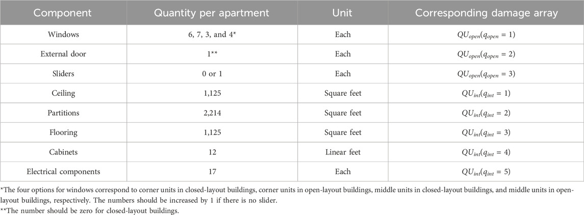
TABLE 1. Quantity of exterior and interior components in an apartment unit.

The repair quantities of exterior and interior components, Q_repair, are the Hadamard product or element-wise product of DR_open and QU_open or DR_int and QU_int, respectively.

where

• ws is the maximum wind speed interval, which ranges from 1 to 41, representing 50 mph to 250 mph with 5 mph width.

• wd is the direction of the maximum wind speed, which ranges from 1 to 8, representing 0 to 315 with 45 width.

• n is the simulation number from 1 to maximum number of simulations. In this study, the maximum number of simulations is 1,000.

• s is the story number, which ranges from 1 to maximum number of stories of the building, S.

• u is the unit number, which ranges from 1 to maximum number of units per story, Us.

• q is the component number: qopen is the exterior component number. qint is the interior component number. q = 1 and q_open = 1 for windows. q = 2 and q_open = 2 for doors. q = 3 and q_open = 3 for sliders. q = 4 and q_int = 1 for ceiling. q = 5 and q_int = 2 for partitions. q = 6 and q_int = 3 for flooring. q = 7 and q_int = 4 for cabinets. q = 8 and q_int = 5 for electrical components.

3.2.2 Definition of repair sequences

Almufti and Willford (2013) defined repair sequences in the REDi^TM Rating System. Figure 2 shows the repair sequences of the components in the WHIP-MHRB vulnerability model, which include demolition and removal, repairs of exterior components (windows, doors, and sliders), and interior components (ceiling, partitions, flooring, cabinets, and electrical components). Here, demolition includes removal based on Plotner (2015).

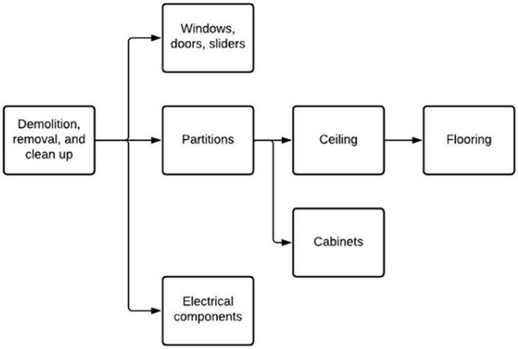
FIGURE 2. Repair sequences per floor.

The demolitions of all damaged components are assumed to start simultaneously. The repairs of exterior components, partitions, and electrical components start simultaneously after the demolition is finished. The repairs of ceilings and cabinets start following the repair of partitions. The repair of flooring follows the repair of ceilings.

The repair of the building starts at the first floor. A specific repair sequence on the sth floor can start after both its predecessor on sth floor and the same repair sequence on (s−1)th floor are finished.

3.2.3 Conversion of repair quantities into unit repair time

Plotner (2008) provided labor hours for different types of construction systems. The labor hours represent the amount of time it takes to install the system per unit of measure. For example, it takes 3.85 h to install a sliding window system (metal clad wood window, 6’×5’, sliding). We assume that a worker works 8 h per day, and the daily output (DO) is the amount of repairs one worker can do in 1 day, which is 8 h divided by the labor hours.

Similarly, Plotner (2015) provided the labor hours for demolition of different components. These are translated to daily output for one worker.

Table 2 provides a summary of the repair daily output and demolition daily output.

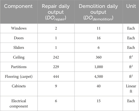
TABLE 2. Repair daily output and demolition daily output for all components.

The unit repair time, TU_repair, for each component is the quantity of damaged component, Q_repair (Eq. 3), divided by the repair daily output, DO_repair, of a specific component (Eq. 4).

The unit demolition and removal time, TUdemolition, for each component is the quantity of damaged component, Q_repair, divided by the demolition daily output, DO_demolition, of a specific component (Eq. 5).

3.2.4 Number of workers needed for repairs

Almufti and Willford (2013) defined the maximum number of simultaneous on-site workers in charge of building repairs, N_max, as a function of total floor area, A_total (Eq. 6). Almufti and Willford (2013) also provided the maximum number of workers per component type as constants for buildings less than 6 stories, between 6 and 20 stories, and greater than 20 stories.

The authors followed the definition of N_max and made adjustments to match the number of workers in repair sequences in this study to those in Almufti and Willford (2013). This study distinguishes the maximum number of workers for windows, doors, and sliders between four different building types: closed-layout buildings with sliders or without sliders and open-layout buildings with sliders or without sliders.

Table 3 shows, as an example, the number of workers for all components in an S-story building for an open-layout building with sliders. The numbers for buildings between 6 and 20 stories come from linear interpolation.

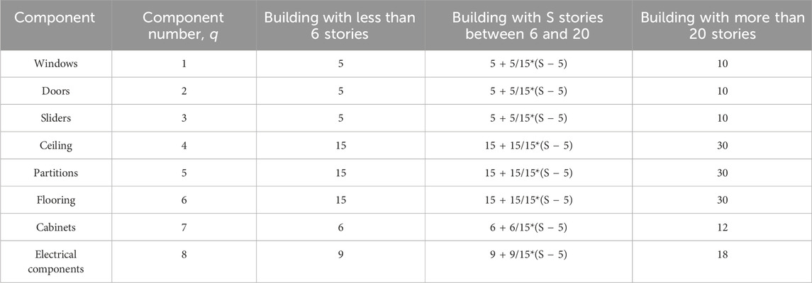
TABLE 3. Maximum number of workers for all components (N_q,max) in an S-story building.

The number of workers for a specific component, N_q, is first set to be the maximum number of workers for that component, N_q,max, as shown in Table 3. q = 1 to 8 represents windows, doors, sliders, ceiling, partitions, flooring, cabinets, and electrical components, respectively. The authors assume that the sum of the numbers of workers for components with the same predecessor (see Figure 2) should be smaller than N_max as a proxy for the number of workers working on site at the same time less than N_max. That is, N₆ (flooring), the sum of N₁ (windows), N₂ (doors), N₃ (sliders), N₅ (partitions), and N₈ (electrical components), and the sum of N₄ (ceiling), and N₇ (cabinets) should each be smaller than N_max. If the sum of N_q is greater than N_max, then N_q should be reduced based on the ratio of N_q,max to the summation. Take windows as an example.

• Assume the summation sum = (N₁ + N₂ + N₃ + N₅ + N₈) is greater than N_max.

• Difference between sum and N_max, Diff = sum − N_max.

• Adjusted N₁, N₁ = N₁ − Diff*(N₁/sum).

The number of workers for the demolition of each component is set to be the same as the number of workers to repair that component.

3.2.5 Critical path concept to the estimate of building repair time

Seal (2001) proposed a spreadsheet-based methodology to implement the program evaluation and review technique/critical path method (PERT/CPM) algorithm (Kelley and Walkerf 1959; Malcolm et al. 1959). PERT/CPM finds the critical path in a project network. The methodology incorporates a matrix (PR_ij) representing the project network (same as the repair sequences, see Figure 2) and the predecessor relationships (for example, partition repair is the predecessor of ceiling repair and cabinet repair). The matrix and relationships are used to produce estimates of Earliest Start (EST), Earliest Finish Time (EFT), Latest Start (LST), and Latest Finish Time (LFT) of the activities and also find the critical path. The WHIP-TRE model takes the maximum EFT of all activities as a proxy for the total repair time of a project.

The repair could start at the first floor or simultaneously on each floor. Due to the limitation of the total number of workers, modeling simultaneous repair would be complicated. To simplify the calculation, the repair of a building is assumed to start at the first story and follow the repair sequences (Figure 2) based on experience and judgment. For the upper stories (story s), due to the limit of the maximum number of workers for a specific repair sequence (sequence t), a predecessor sequence (sequence t) on the lower story (story s−1) should be incorporated. The resulting matrix, denoted as PR₁, illustrates the project network and the predecessor relationships of all repair sequences as shown in Table 4. The predecessor column lists the predecessor sequence of a specific sequence. For example, for sequence 3 (door repair), the predecessor sequence is sequence 1 (demolition). For sequence 6 (ceiling repair), the predecessor sequence is sequence 5 (partitions).

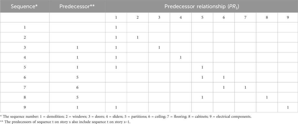
TABLE 4. Matrix of the project network and predecessor relationships of all repair sequences.

The meaning of each repair sequence t = 1 to 9 is explained below the table. Since the predecessor sequence should have a smaller index based on Seal (2001), we exchange the index of ceiling (q = 4 to q = 5) and partitions (q = 5 to q = 4). For the first story, the relationship matrix, denoted as PR₀, should be the PR₁ minus an identity matrix to replace the diagonal entries to 0.

The repair time (T_repair) of repair sequence t on story s is the sum of repair time (TU_repair) of sequence t for each apartment u on story s divided by the number of workers for sequence t (N_q = t − 1). We assume that the demolition of all damaged components for a given story start at the same time; therefore, the repair time of demolition (t = 1) is the maximum of the sum of demolition time (TU_demolition) for each apartment u and then divided by the number of demolition (N_q = t − 1).

Equations 7 and 8 provide the estimate of the repair time of repair sequence t on story s given a combination of ws, wd, and simulation (T_repair).

This methodology estimates the EST and EFT in sequence from the first repair sequence (t = 1) on the first story (s = 1) to the last repair sequence (t = 9) on the first story (s = 1), then to t = 1 and s = 2, so on and so forth, to calculate the repair time of the building (Trepair_building).

First, the arrays EST(ws, wd, n, t) and EFT(ws, wd, n, t) are initialized with all zeros. Equation 9 illustrates the estimate of EST of repair sequence t on the first story, which is the maximum value of the products of EFT given t = j and the element in the tth row and jth column with j ranging from 1 to 9.

Equation 10 illustrates the estimate of EFT of repair sequence t on story s, which is the EST of repair sequence t plus the repair time of that repair sequence on story s.

Equation 11 describes the estimate of EST for the repair sequences above the first story.

The repair time of the building equals the EFT of the last repair sequence (t = 9) on the highest story (s = S) (Eq. 12):

3.3 Estimate of delay time

The WHIP-TRE model estimates delay time due to the inspection, engineering mobilization and review, financing, contractor mobilization, and permitting after hurricane events. This method leverages the impeding curves (see Section 2) from Almufti and Willford (2013) combined with certain assumptions based on engineering judgment to produce reasonable estimates of delay time.

The mean delay time is a function of the physical damage ratio of interior (DR_int) or exterior (DR_ext) components of the building after DR_int or DR_ext exceeds a threshold DR0. Observations and engineering judgment result in a wind damage ratio threshold equivalent to the seismic repair class (RC) threshold in the REDi^TM system. Simply speaking, RC = 1, 2, and 3 represent minor, medium, and severe damage, respectively. This lowest damage ratio DR0 triggers a non-zero delay time. The computation of the delay times in the WHIP-TRE model works as follows:

1. Convert the seismic RC into an equivalent wind $(\overline{DR})$ based on detailed description of damage conditions of RC (Almufti and Willford, 2013) and authors’ judgment: seismic threshold RC = 1 corresponds to wind DR0 = 30%; seismic threshold RC = 3 corresponds to wind DR0 = 70%. When DR > DR0, the delay time is greater than zero. If not, the delay time is zero.

2. Define the maximum mean delay time T_max based on the selected impeding curve. Almufti and Willford (2013) provided impeding curves for different building types and other conditions. Researchers can choose the curves of interest. Assume on the impeding curve that the time with the probability of exceedance of 100% (for inspection) or 95% (for others) is T_max. Then, assume that when $\overline{DR}=1$, the mean delay time is T_max. Figure 3 shows an impeding curve, for example, for delay time of inspection, where the probability of non-exceedance refers to the probability that inspection will exceed the time value on the abscissa.

3. Use Eq. 13, derived from engineering judgment, to calculate mean delay time as a function of $\overline{DR}$.

4. Assign delay time for each MC simulation based on a Poisson distribution with a mean value equal to the calculated mean delay time from Eq. 13. Table 5 lists the values of the variables for different delay factors in this equation.

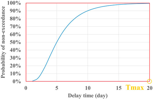
FIGURE 3. Impeding curve for inspection.

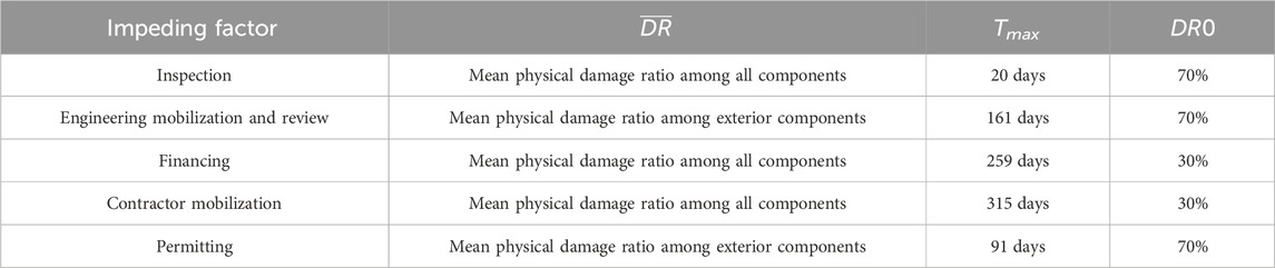
TABLE 5. Values of key variables in delay time estimation.

Based on Almufti and Willford (2013), impeding curves of engineering mobilization and review and permitting are applied when structural damage, for example, floor damage or external wall damage, is greater than a certain threshold. In addition, the WHIP-MHRB model assumes that there is no structural damage in MHRB during hurricane events (all damage occurs to openings and from water ingress), so the WHIP-TRE model does not incorporate the delay due to engineering mobilization and review or permitting for MHRB.

Similar to repair sequences, this method also leverages the delay time sequences from Almufti and Willford (2013). The delay due to inspection will come first after a hurricane event. The delay due to financing, engineering mobilization and review, and contractor mobilization come simultaneously after the delay due to inspection. The delay due to permitting will come after the delay due to engineering mobilization and review.

Based on this delay time sequences, the program computes the total delay time (Tdelay) for each MC simulation as follows:

Currently, in the WHIP-TRE model, Tdelay_engineering and Tdelay_permitting are set to 0 for MHRB.

3.4 Estimate of downtime

The methodology addresses the downtime due to the disruption of electrical power networks and is a function of WS_max. Downtimes due to disruptions of other utilities such as communication systems (for example, cellular phone network and internet) and transportation (bridges, roads, signs, and gas stations) will be added to the model later based on further research studies.

Reed et al. (2010b), Reed et al. (2010a), and Powell et al. (2010) proposed a quality function Q(t) for Hurricane Rita and Hurricane Katrina. The quality function quantifies the time for electric power restoration after an event and is equal to 100% for a fully functioning system. It took 20 and 48 days for the power grid to be totally restored after Hurricane Rita and Hurricane Katrina, respectively.

Knabb et al. (2005) and Knabb et al. (2006) recorded the maximum surface wind speeds for several power stations during the two hurricanes. The maximum 3-s gust wind at 10 m height over open terrain was 116 mph and 135 mph for Hurricane Rita and Hurricane Katrina, respectively. This research assumes that the most serious damage, which results in the longest outage, occurs at the highest wind speed. The results are combinations of actual terrain 3-s wind speed at 10 m and downtime due to disruption of power grids: 116 mph leading to 20 days downtime (Hurricane Rita) and 135 mph leading to 48 days downtime (Hurricane Katrina). Moreover, 50 mph corresponds to 0 days downtime.

Figure 4 shows the polynomial regression through these three points that leads to Eq. 15, which gives the mean downtime of the power grid $(\stackrel{̄}{T_{dow{n}_{\mathit{electricity}}}})$. $\stackrel{̄}{T_{dow{n}_{\mathit{electricity}}}}$ is assumed to be a constant 48 days when WS_max is greater than 135 mph (60.35 m/s). Matched hazard intensities and downtimes due to disruption of power grids will be collected to improve this function.

where a₀ = 8.15937247, a₁ = −0.50520292, a₂ = 0.01220515, a₃ = −0.00014306, and a₄ = 0.00000072. The unit of WS_max is mph in this function.

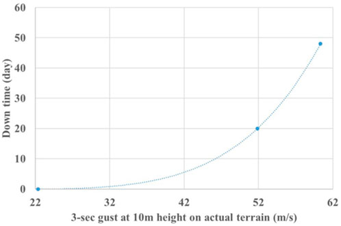
FIGURE 4. Power grid downtime as a function of WS_max.

Although the estimate of downtimes due to other utility system disruptions is not currently available, we assume that the restoration of all utility systems occurs simultaneously after a hurricane event. Therefore, the total downtime (Tdown) would be the maximum of the downtimes due to the disruption of each utility network.

3.5 Estimate of recovery time

The authors converted the time framework proposed by Almufti and Willford (2013) for full recovery after an earthquake into the one for full recovery after a hurricane event. Based on this time framework, Eq. 16 defines the recovery time (Treco) as follows:

3.6 TRE conversion

The TRE of apartment building owners are covered by business income insurance (BIC) policies.

For BIC, the model assumes that the policy will cover up to 365 days of the loss of the rent for an apartment building owner based on the FCHLPM actuarial standard (FCHLPM, 2021). Equation 17 defines the TRER for BIC:

Since condo unit owners or renters can reoccupy their apartments after the whole building is repaired, the WHIP-TRE model can be expanded to two different types of TRE for MHRB: ALE of condominium owners (HO-6 policy in the US insurance market) and ALE of renters (HO-4 policy).

Different insurance companies may determine their own daily expenses TRE_daily and overall TRE coverage TRE_total. For HO-4 and HO-6, the insurance covers the cost of lodging, meals, and incidental expenses (M&IE) if the residents need to be relocated after a hurricane event. Federal agencies use per diem rates (PDR) to reimburse their employees for subsistence expenses incurred while on official travel. The General Services Administration (2023) provides the PDR for different states and counties. Since most of the continental United States (CONUS) is covered by the standard per diem rate of $157 ($98 lodging and $59 M&IE), the model adopts the following for HO-4 and HO-6 (Eq. 18):

Typically, the coverage limits of ALE for HO-4 and HO-6 are 30% and 50% of the personal property limit, respectively (Avner Gat Inc, 2019). Personal property coverage protects the contents inside the apartment. The personal property is usually 50%–70% of the dwelling limit (Moon, 2023), assumed to be 60% of an apartment unit cost in the model. The cost of an apartment unit equals the unit cost multiplied by the apartment area (1125 sf). We assume that the unit cost of a property is $137 per square foot derived from the RSMeans dataset. The resulting TRE_total are calculated from (Eq. 19)

Equation 20 defines the TRER for HO-4 and HO-6:

4 WHIP-TRE model outputs

For each building class, the outputs of the WHIP-TRE model include the time and TRE vulnerability matrices (for the repair times, delay times, downtimes, and recovery times) conditional on either WS_max or DR_Bldg [see (Wei et al., 2023) for more details]. The model also produces time and TRE vulnerability curves, which represent the mean times and TRER conditional on WS_max or DR_Bldg, derived from the time and TRE vulnerability matrices. These outputs are discussed below.

4.1 Time vulnerability matrices

In the time vulnerability matrices V(TIME, WS_max) and V(TIME, DR_Bldg), each cell is the probability that the duration for a certain process, conditional on either WS_max or DR_Bldg, will be in a given interval, to shown in Eqs 21, 22:

We simplify the notation to shown in Eqs 23a, 23b:

where

• [time_k, time_k+1] is the kth time interval, represented as TIME = time_k. We define 53 7-day time intervals from 0 days to 364 days. In this research, we assume that the insurance policy will cover up to 365 days of the loss of the rent for an apartment building owner (see Section 3.6).

• [ws_i, ws_i+1] is the ith WS_max interval, represented as WS_max = ws_i. We define 41 wind speed intervals from 50 mph (22.35 m/s) to 250 mph (111.76 m/s) with a 5 mph (2.24 m/s) width.

• [dr_l, dr_l+1] is the lth DR_Bldg interval, represented as DR_Bldg = dr_l. We define 21 damage ratio intervals from 0% to 100% with a 4.76% width.

• $n_{tim{e}_k,w{s}_i}$ is the number of simulations in the time interval TIME = time_k, with WS_max in the interval WS_max = ws_i.

• $n_{w{s}_i}$ is the number of simulations in the WS_max interval WS_max = ws_i.

• $n_{tim{e}_k,d{r}_l}$ is the number of simulations in the time interval TIME = time_k, with DRBldg in the interval DR_Bldg = dr_l.

• $n_{d{r}_l}$ is the number of simulations in the DR_Bldg interval DR_Bldg = dr_l.

Each column of the matrices provides the discretized probability distribution function of time conditional on WS_max or DR_Bldg, where

• TIME ranges from 0 day to 364 days at a 7-day interval, with each row of the matrices representing the minimum value of the time interval.

• WS_max ranges from 50 mph to 250 mph at a 5-mph interval, with each column of the matrices representing the middle point of the wind speed interval.

• DR_Bldg ranges from 0% to 100% at a 4.76% interval, with each column of the matrices representing the minimum value of the wind speed interval.

4.2 Time vulnerability curves

The matrices V(TIME, WS_max) and V(TIME, DR_Bldg) yield the time vulnerability curves for recovery time, repair time, delay time, or downtime $\overline{TIME}(W{S}_{\mathit{max}})$ and $\overline{TIME}(D{R}_{\mathit{Bldg}})$. The vulnerability curve represents the mean duration for a given process conditional on WS_max or DR_Bldg calculated with Eqs 24 and 25, respectively, where treco representing recovery time can be replaced by trepair, tdelay, and tdown for repair time, delay time, and downtime, respectively.

Figure 5A shows three examples of $\overline{treco}(W{S}_{\mathit{max}})$ and Figure 5B shows three examples of $\overline{treco}(D{R}_{\mathit{Bldg}})$ for the building classes:

• ABTI_open_U6_S6_YSD_Nsh_C

• ABTI_open_U6_S11_YSD_Nsh_C

• ABTI_open_U6_S16_YSD_Nsh_C

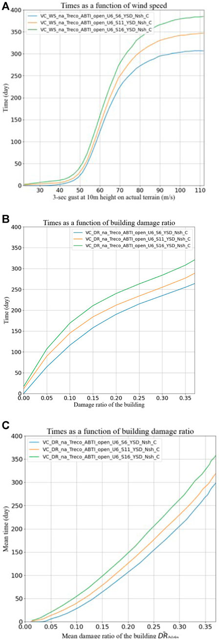
FIGURE 5. Examples of $\overline{treco}(W{S}_{\mathit{max}})$ (A), $\overline{treco}(D{R}_{\mathit{Bldg}})$ (B), and $\overline{treco}(\overline{D{R}_{\mathit{Bldg}}})$ (C).

These building classes represent 6/11/16-story apartment buildings with six apartments per story, open layout (apartment accessed externally), with slider, standard glass windows without shutters, and carpet flooring. The only different building parameter among these building classes is the number of stories. The taller a building, the more the apartments, resulting in longer repair times.

The first DR_Bldg interval contains points with damage ratios ranging from 0% to 4.76%. In this interval, when the damage ratio of an apartment is greater than 0%, the repair time for this apartment is small but greater than 0 day resulting in non-zero recovery time. In the same way, the aggregation repair time for tall buildings is greater than that for short buildings. The mean recovery time of these points is plotted in Figure 5B at DR_Bldg equal to 0%, so the mean recovery time does not start from 0 days.

Alternatively, this study also adapted the methodology proposed by Barbato et al. (2013) for the conversion of time vulnerability as a function of WS_max, $\overline{TIME}(W{S}_{\mathit{max}})$, into time vulnerability as a function of the mean building damage ratio $\overline{D{R}_{\mathit{Bldg}}}$, $\overline{TIME}(\overline{D{R}_{\mathit{Bldg}}})$ [see also (Paleo-Torres et al., 2020)]. The building vulnerability curve $\overline{D{R}_{\mathit{Bldg}}}$ is derived from the building vulnerability matrix [where each cell represents the probability of having DR_Bldg given WS_max; see (Wei et al., 2023) for more information]. For each value of WS_max, the corresponding pair of $\overline{TIME}(W{S}_{\mathit{max}})$ and $\overline{D{R}_{\mathit{Bldg}}}(W{S}_{\mathit{max}})$ results in the function $\overline{TIME}(\overline{D{R}_{\mathit{Bldg}}})$. Figure 5C shows examples of $\overline{treco}(\overline{D{R}_{\mathit{Bldg}}})$ for the same building classes shown in Figure 5B.

It is clear from the figures that $\overline{treco}(\overline{D{R}_{\mathit{Bldg}}})$ is different from $\overline{treco}(D{R}_{\mathit{Bldg}})$. $\overline{treco}(D{R}_{\mathit{Bldg}})$ represents the mean recovery time for any possible damage ratio of the building. $\overline{treco}(\overline{D{R}_{\mathit{Bldg}}})$ is the mean recovery time for the expected damage ratio of the building at every WS_max. If a building suffers damage equal to DR_Bldg during a hurricane, $\overline{treco}(D{R}_{\mathit{Bldg}})$ shall provide an estimate of its expected recovery time, regardless of the wind speed that caused the damage. However, if the damage to a building subjected to a known WS_max is unknown, the building vulnerability curve can provide a value for the expected damage ratio, and $\overline{treco}(\overline{D{R}_{\mathit{Bldg}}})$ shall provide an estimate of its expected recovery time. For validation purposes, both curves can be used depending on the circumstances.

4.3 TRE vulnerability matrices and curves

Section 3.6 shows how the different duration times can be converted into corresponding TRE. Consequently, the matrices V(TIME, WS_max) and V(TIME, DR_Bldg) can be converted into TRE vulnerability matrices V(TRER, WS_max) and V(TRER, DR_Bldg), which yield the TRE vulnerability curves $\overline{TRE}(W{S}_{\mathit{max}})$ and $\overline{TRE}(D{R}_{\mathit{Bldg}})$, respectively.

V(TRER, WS_max) or V(TRER, DR_Bldg) are identical to V(TIME, WS_max) or V(TIME, DR_Bldg), respectively, except that each row time interval in the TIME matrices is translated into a row TRE interval in TRER matrices based on Eq. 17 in Section 3.5.

The TRE vulnerability curves $\overline{TRE}(W{S}_{\mathit{max}})$ and $\overline{TRE}(D{R}_{\mathit{Bldg}})$ are also identical to $\overline{TIME}(W{S}_{\mathit{max}})$ and $\overline{TIME}(D{R}_{\mathit{Bldg}})$, respectively, except for the scaling of the vertical axis from TIME into TRE. The vulnerability curve is the mean TRER conditional on WS_max or DR_Bldg calculated with Eqs 26 and 27, respectively.

where trer_k is the kth TRER interval transformed from the kth TIME interval based on Section 3.6.

Figures 6A, B show examples of $\overline{TRE}(W{S}_{\mathit{max}})$ and $\overline{TRE}(D{R}_{\mathit{Bldg}})$ for building classes:

• VC_WS_na_TRE_ABTI_open_U6_S11_YSD_Nsh_C

• VC_DR_na_TRE_ABTI_open_U6_S11_YSD_Nsh_C

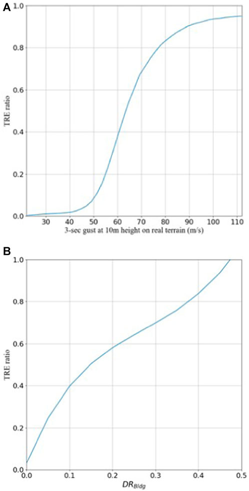
FIGURE 6. Examples of $\overline{TRE}(W{S}_{\mathit{max}})$ (A) and $\overline{TRE}(D{R}_{\mathit{Bldg}})$ (B).

These building classes represent 11-story apartment buildings with six apartments per unit, open layout (apartment accessed externally), with slider, standard glass windows without shutters, and carpet flooring. TRER and treco are linearly related (see Section 3.6).

5 Logical relationships to risk

This section produces sample results from the WHIP-TRE model and displays them in pairs to test the logical relationships to risk (LRR) of this model’s output.

The Florida Commission on Hurricane Loss Projection Methodology (FCHLPM), standard A-6 (FCHLPM, 2021) requirements which apply to actuarial loss can be extended to vulnerability as follows: “Modeled hurricane vulnerabilities should vary according to risk. If the risk of damage due to hurricanes is higher for one building class, then the hurricane vulnerability should also be higher. Likewise, if there is no difference in risk, there should be no difference in hurricane vulnerability. Hurricane vulnerabilities not having these properties do not have a logical relationship to risk.” We can further extend this concept to the recovery time due to hurricane damage.

The expected logical relationships to risk as they apply to the duration of different processes and TRE are listed as follows: the increase in wind speed leads to more serious damage to a building, resulting in longer recovery time. Similarly, a higher level of window protection and a change from open layout to closed layout leads to less water ingress and interior damage, resulting in shorter recovery time. A taller building has more damaged apartments to be repaired, which requires a longer recovery time.

Several building classes were selected to verify the logical relationships to risk of the model vulnerability outputs. The building classes are shown in Table 6. The building class ABTI_open_U6_S10_YSD_Nsh_C (insurance for funding, open layout, 6 units per story, 10 stories, with slider, no shutter, and carpet floor) was selected as a benchmark building class. Five other building classes were chosen to investigate the impact of the selected key parameters (window protections, building layouts, and number of stories). The parameters include the window protection (Nsh for no shutter and Ysh for with metal shutter), layout (open and closed for apartment units accessed externally and internally), and number of stories (S5, S10, and S15 for 5/10/15-story buildings).

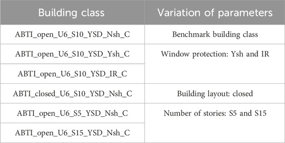
TABLE 6. Selected time building classes for the LRR test of the WHIP-TRE model.

The WHIP-TRE model generates $\overline{TIME}(W{S}_{\mathit{max}})$, where time can be treco, trepair, tdelay, and tdown (based on 1,000 MC simulations) for each of the six building classes of Table 6. Due to space limitation, this section only illustrates vulnerability curves for treco and the selected parameters. These are plotted in Figure 7.

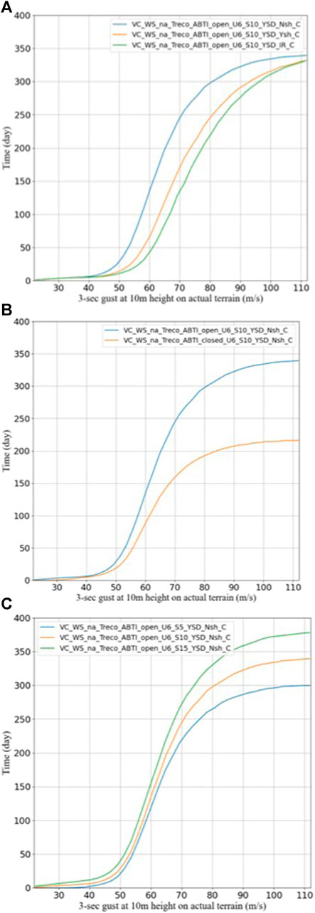
FIGURE 7. Comparisons of vulnerability curves for recovery times with different window protections (A), building layouts (B), and number of stories (C).

These figures show that a higher level of window protection results in a decrease in treco; that open buildings are more vulnerable than closed buildings resulting in longer recovery times (recall open buildings have entry doors to the individual units that are directly exposed to the outside, while closed buildings have units with entry doors exposed to an interior common space); and that higher buildings with more damaged apartments require longer recovery time. These results of the WHIP-TRE model satisfy the logical relationship to risk requirement.

Although the model replicates the expected relationships to risk, claims data are still needed to evaluate the accuracy of these risk-consistent outputs.

6 Comparison between the WHIP-TRE model and HAZUS-MH Hurricane Model

The scarcity of quality claims data is a problem for all modelers who develop MHRB catastrophe models since it hinders validation and calibration. In that context, all models contain a substantial amount of engineering judgment. For example, the widely used catastrophe model, HAZUS-MH Hurricane Model, developed its economic loss module for commercial buildings (including MHRB) primarily based on experience and judgment, with limited calibration (FEMA, 2022b).

Assuming that all models are based on sound engineering science, judgment, and experience, it is difficult to evaluate whether one model is superior to another, given the degree of uncertainty present in each model and the absence of actual claims data. However, it is useful for model developers and users to compare the results from different models to gauge the range of uncertainty of the projected losses and the influence of assumptions, interpretations, strategies, and parameter settings that differ between models. In this section, the results of the WHIP-TRE model are compared to those of the HAZUS-MH Hurricane Model.

The HAZUS-MH Hurricane Model provides the expected number of days needed to restore the utility of each building type as a function of peak gust wind speed at 10 m height over open terrain. These loss-of-use functions vary according to the type of terrain, roof cover type, window area, opening protection, and wind debris.

The authors extracted certain loss-of-use functions from HAZUS-MH Hurricane Models and compared these to the equivalent time vulnerability curves from the WHIP-TRE model. The comparisons are shown in Figure 8.

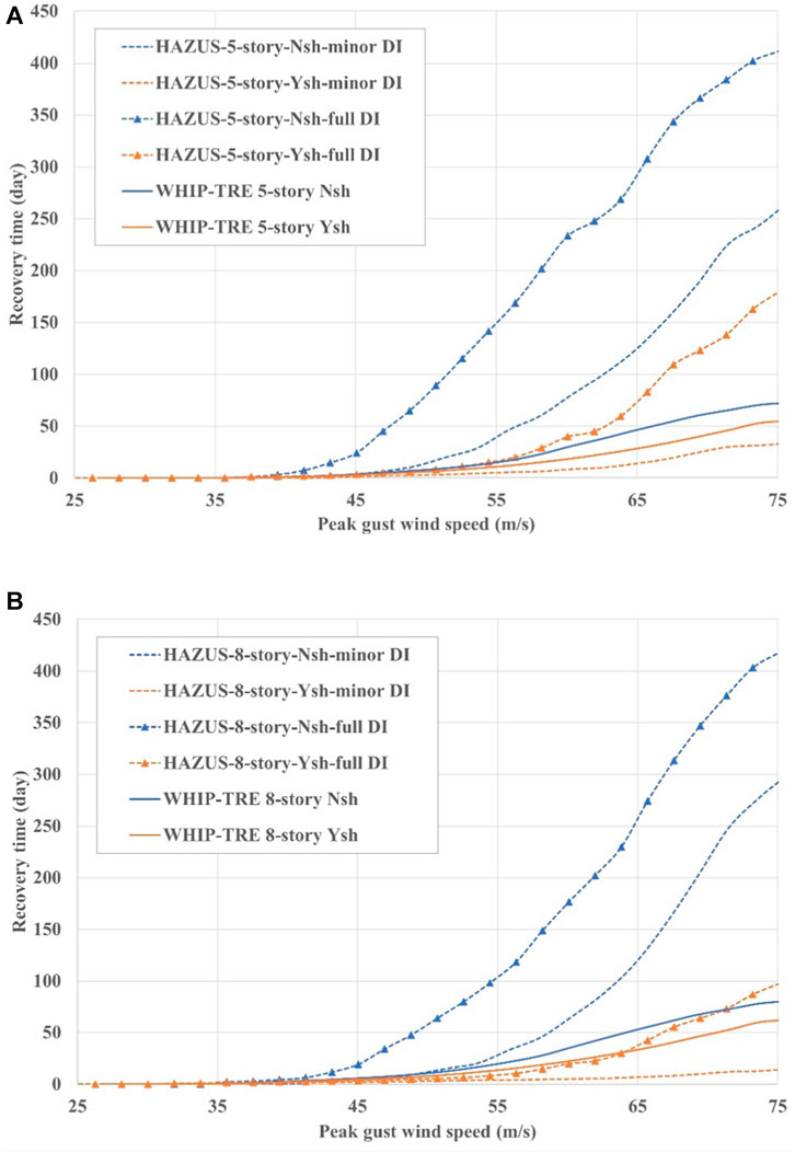
FIGURE 8. Comparisons of recovery time vulnerability curves for 5-story buildings (A) and 8-story buildings (B).

The key parameters of the selected loss-of-use functions and time vulnerability curves are listed in Table 7. For the HAZUS-MH loss-of-use functions, regardless of the actual terrain, the independent variable is peak gust wind speed at 10 m height over open terrain. In the WHIP-TRE model, the recovery time is a function of peak gust wind speed at 10 m height over the actual terrain where the building is located. For compatibility purposes, for the case of the HAZUS-MH loss-of-use functions for suburban buildings, the authors converted the wind speeds over open terrain into wind speeds over suburban terrain based on the wind speed conversion factors from FEMA (2022b).

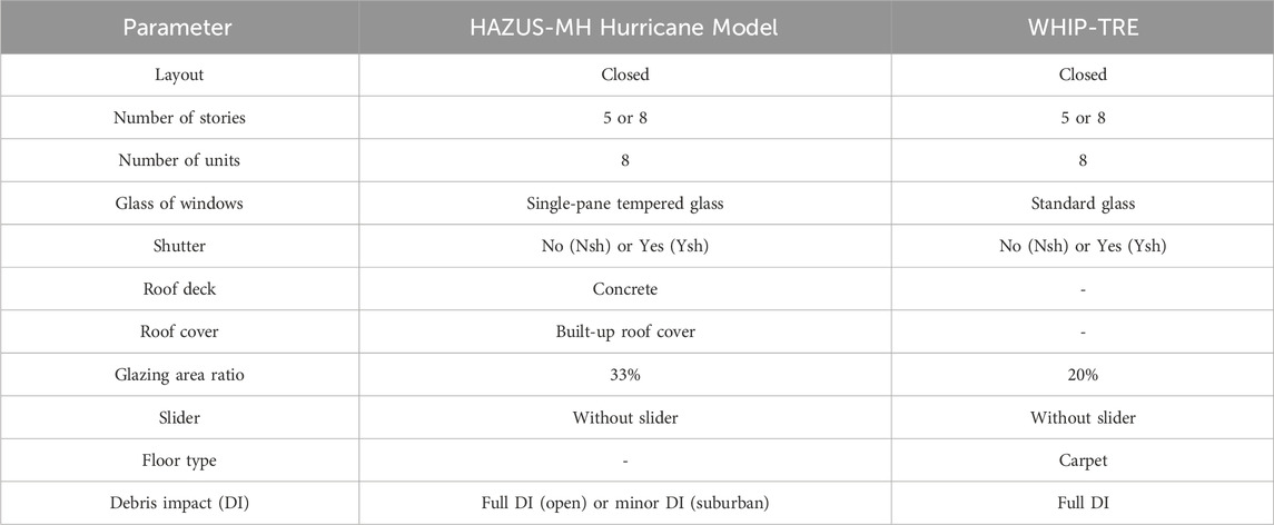
TABLE 7. Key parameters for loss-of-use functions from the HAZUS-MH Hurricane Model and time vulnerability curves from WHIP-TRE.

There is an obvious difference between the HAZUS loss-of-use functions with full debris impact (DI) and minor DI. The WHIP-TRE time vulnerability curves are in the range of the loss-of-use functions with minor DI for 5-story and 8-story buildings with and without shutters.

Shutters have a greater impact on the results of HAZUS-MH than on the WHIP-TRE model.

The recovery times from HAZUS-MH is a function of damage ratio of the building, so for some given wind speeds, the recovery time for a 5-story building is greater than that for an 8-story building where the damage ratio of the building is the same (Wei et al., 2023).

Due to the absence of claims data, it is not possible to evaluate the relative accuracy of the models, other than to say they both exhibit a logical relationship with the additional vulnerability associated with a high debris impact environment and the use of opening protection. The impact of DI and shutters on the recovery time for MHRB is an obvious target for further investigation and a topic of claims data analysis when available.

7 Conclusion

The WHIP-TRE model combines building damage estimates from the WHIP-MHRB vulnerability model with explicit estimates of repair times, delay times, and downtimes, leading to a realistic TRE model for MHRB. This WHIP-TRE methodology can be extended to estimate TRE for low-rise buildings and possibly to hazards other than hurricanes.

The WHIP-TRE model outputs the mean estimate of recovery time as a function of the wind speed or damage ratio of the building. The model also converts different times into TRE ratio. These results should be more realistic than results of many existing TRE models since they include repair sequences, delay due to different factors (such as post hurricane inspection, financing, contractor mobilization, and permitting), and downtimes due to disruption of utilities.

Insurers can convert the outputs into TRE ratios based on their own specification in terms of daily TRE and total TRE coverage. Modelers or insurers can replace the impeding curves for delay factors or utility disruption functions to test the impact on the recovery time of different scenarios with varying delay assumptions, or more or less vulnerable utilities. Due to the event-based nature of the combined WHIP-MHRB and WHIP-TRE models, modelers can also test the impact of mitigation measures on recovery times and TRE. The model can be used for resilience studies since recovery times are a good measure of community resilience.

The authors verified that the model outputs follow logical relationships to risk, but a remaining issue in TRE model validation and calibration for MHRB is a lack of quality insurance claims data. This is a problem for all MHRB TRE models. Claims data usually do not include recovery times, making validation even more challenging. Surveys for MHRB after hurricanes are necessary to gather actual recovery times.

Considering the lack of claims data for validation, the paper compares curves of recovery times from the HAZUS-MH Hurricane Model and the WHIP-TRE model. The HAZUS-MH model is much more sensitive to debris impact and the existence of window protection than the WHIP-TRE model. The WHIP-TRE model tends to predict similar recovery times compared to the HAZUS-MH model for low and medium wind speeds and relatively less recovery time at high wind speeds.

In this research, the authors made some assumptions in prediction of repair times. For example, the repair of damaged buildings is currently assumed to start from the first floor. Other options could be considered. The methodology to estimate delay time and downtime is extrapolated from a seismic model. Delay time and downtime functions derived from hurricane data are needed to improve the model. Finally, current deterministic variables of the TRE model and their contribution to the overall uncertainty of the model evaluated could be treated stochastically.

Data availability statement

The data are not publicly available because the research was funded by WHIP Center and any data distribution requires the pre-approval of the Center’s Leadership Team.

Author contributions

ZW: Conceptualization, Formal Analysis, Investigation, Software, Writing–original draft. J-PP: Funding acquisition, Supervision, Writing–original draft, Writing–review and editing. KG: Supervision, Writing–original draft, Writing–review and editing. SH: Project administration, Validation, Writing–review and editing. GF: Validation, Writing–review and editing.

Funding

The author(s) declare financial support was received for the research, authorship, and/or publication of this article. The National Science Foundation supports the Center for Wind Hazard and Infrastructure Performance (WHIP-C) through grant numbers IIP 1841503 and 1841523, and the Industrial Advisory Board of the WHIP-C supported this work through grant number WHIP2021_P05. The Florida Office of Insurance Regulation (FOIR) also supported part of this work through grant number 000429.

Acknowledgments

The opinions, findings, and conclusions presented in this paper are those of the author alone and do not necessarily represent the views of the NSF or the WHIP-C or the FOIR.

Conflict of interest

Author GF was employed by AMI Risk Consultants, Inc.

The remaining authors declare that the research was conducted in the absence of any commercial or financial relationships that could be construed as a potential conflict of interest.

The author(s) declared that they were an editorial board member of Frontiers, at the time of submission. This had no impact on the peer review process and the final decision.

Publisher’s note

All claims expressed in this article are solely those of the authors and do not necessarily represent those of their affiliated organizations, or those of the publisher, the editors, and the reviewers. Any product that may be evaluated in this article, or claim that may be made by its manufacturer, is not guaranteed or endorsed by the publisher.

References

AIR (AIR Worldwide Corporation) (2021). Standards of the Florida commission on hurricane loss projection methodology.
ARA (Applied Research Associates) (2021). HurLoss version 10.0 Florida commission on hurricane loss projection methodology 2019 hurricane standards. 10.0.
Barbato, M., Petrini, F., Unnikrishnan, V. U., and Ciampoli, M. (2013). Performance-based hurricane engineering (PBHE) framework. Struct. Saf. 45, 24–35. doi:10.1016/J.STRUSAFE.2013.07.002
Biasi, G., Eeri, M., Mohammed, M. S., and Sanders, D. H. (2017). Earthquake damage estimations: ShakeCast case study on Nevada bridges. Earthq. Spectra 33, 45–62. doi:10.1193/121815EQS185M
Chian, S. C. (2016). A complementary engineering-based building damage estimation for earthquakes in catastrophe modeling. Int. J. Disaster Risk Sci. 7, 88–107. doi:10.1007/s13753-016-0078-5
Chuang, W. C., and Spence, S. M. (2017). A performance-based design framework for the integrated collapse and non-collapse assessment of wind excited buildings. Eng. Struct. 150, 746–758. doi:10.1016/j.engstruct.2017.07.030
CoreLogic (2021). Florida hurricane model 2021a A component of the CoreLogic north atlantic hurricane model in risk quantification and engineering tm v21 Florida commission on hurricane loss projection methodology. Tech. rep.
Dong, W. (2002). Engineering models for catastrophe risk and their application to insurance. Earthq. Eng. Eng. Vib. 1, 145–151. doi:10.1007/s11803-002-0018-9
FCHLPM (2021). Hurricane standards Report of activities as of november 1, 2021 Florida commission on hurricane loss projection methodology. Tech. rep.
Hamid, S., Golam Kibria, B. M., Gulati, S., Powell, M., Annane, B., Cocke, S., et al. (2010). Predicting losses of residential structures in the state of Florida by the public hurricane loss evaluation model. Stat. Methodol. 7, 552–573. doi:10.1016/j.stamet.2010.02.004
Hamid, S. S., Pinelli, J. P., Chen, S. C., and Gurley, K. (2011). Catastrophe model-based assessment of hurricane risk and estimates of potential insured losses for the State of Florida. Nat. Hazards Rev. 12, 171–176. doi:10.1061/(ASCE)NH.1527-6996.0000050
Hatzikyriakou, A., and Lin, N. (2016). Impact of performance interdependencies on structural vulnerability: a systems perspective of storm surge risk to coastal residential communities. Reliab. Eng. Syst. Saf. 158, 106–116. doi:10.1016/j.ress.2016.10.011
IF (Impact Forecasting) (2021). Impact forecasting Florida hurricane model version 1.0 ELEMENTS version 15.0. Tech. rep.
Kelley, J. E., and Walkerf, M. R. (1959). “Critical-path planning and scheduling”, in PROCEEDINGS OF THE EASTERN JOINT COMPUTER CONFERENCE.
Knabb, R. D., Brown, D. P., and Rhome, J. R. (2006). Tropical cyclone Report hurricane Rita. Tech. rep.
Knabb, R. D., Rhome, J. R., and Brown, D. P. (2005). Tropical cyclone Report hurricane Katrina. Tech. rep.
Ma, L., Christou, V., and Bocchini, P. (2021). Framework for probabilistic simulation of power transmission network performance under hurricanes. Reliab. Eng. Syst. Saf. 217, 108072. doi:10.1016/j.ress.2021.108072
Malcolm, D. G., Roseboom, J. H., Clark, C. E., and Fazar, W. (1959). Application of a technique for research and development program evaluation. Operations Res. 7, 646–669. doi:10.1287/OPRE.7.5.646
Michel-Kerjan, E., Hochrainer-Stigler, S., Kunreuther, H., Linnerooth-Bayer, J., Mechler, R., Muir-Wood, R., et al. (2013). Catastrophe risk models for evaluating disaster risk reduction investments in developing countries. Risk Anal. 33, 984–999. doi:10.1111/j.1539-6924.2012.01928.x
Paleo-Torres, A., Gurley, K., Pinelli, J. P., Baradaranshoraka, M., Zhao, M., Suppasri, A., et al. (2020). Vulnerability of Florida residential structures to hurricane induced coastal flood. Eng. Struct. 220, 111004. doi:10.1016/J.ENGSTRUCT.2020.111004
Pinelli, J. P., Gurley, K. R., Subramanian, C. S., Hamid, S. S., and Pita, G. L. (2008). Validation of a probabilistic model for hurricane insurance loss projections in Florida. Reliab. Eng. Syst. Saf. 93, 1896–1905. doi:10.1016/J.RESS.2008.03.017
Pinelli, J.-P., Pita, G., Gurley, K., Torkian, B., Hamid, S., and Subramanian, C. (2011). Damage characterization: application to Florida public hurricane loss model. Nat. Hazards Rev. 12, 190–195. doi:10.1061/(ASCE)NH.1527-6996.0000051
Powell, M. D., Murillo, S., Dodge, P., Uhlhorn, E., Gamache, J., Cardone, V., et al. (2010). Reconstruction of Hurricane Katrina’s wind fields for storm surge and wave hindcasting. Ocean. Eng. 37, 26–36. doi:10.1016/J.OCEANENG.2009.08.014
Reed, D. A., Asce, M., Powell, M. D., and Westerman, J. M. (2010a). Energy supply system performance for hurricane Katrina. J. Energy Eng. 136, 95–102. doi:10.1061/ASCEEY.1943-7897.0000028
Reed, D. A., Powell, M. D., and Westerman, J. M. (2010b). Energy infrastructure damage analysis for hurricane Rita. Nat. Hazards Rev. 11, 102–109. doi:10.1061/(ASCE)NH.1527-6996.0000012
Seal, K. C. (2001). A generalized PERT/CPM implementation in a spreadsheet. Inf. Trans. Educ. 2, 16–26. doi:10.1287/ited.2.1.16
Wang, S., and Reed, D. A. (2017). Vulnerability and robustness of civil infrastructure systems to hurricanes. Front. Built Environ. 3. doi:10.3389/fbuil.2017.00060
Keywords: time-related expenses, hurricane damage, probabilistic vulnerability model, recovery time, additional living expenses, business interruption insurances, resilience
Citation: Wei Z, Pinelli J-P, Gurley K, Hamid S and Flannery G (2024) Component-based estimation of recovery time and time-related expenses after hurricane events. Front. Built Environ. 9:1295619. doi: 10.3389/fbuil.2023.1295619
Received: 16 September 2023; Accepted: 18 December 2023;
Published: 12 January 2024.
Edited by:
Pedro L. Fernández-Cabán, Florida A&M University—Florida State University College of Engineering, United StatesReviewed by:
Wanting (Lisa) Wang, Colorado State University, United StatesSeymour M. J. Spence, University of Michigan, United States
Copyright © 2024 Wei, Pinelli, Gurley, Hamid and Flannery. This is an open-access article distributed under the terms of the Creative Commons Attribution License (CC BY). The use, distribution or reproduction in other forums is permitted, provided the original author(s) and the copyright owner(s) are credited and that the original publication in this journal is cited, in accordance with accepted academic practice. No use, distribution or reproduction is permitted which does not comply with these terms.
*Correspondence: Zhuoxuan Wei, weiz2018@my.fit.edu