Semi-Stochastic Gradient Descent Methods
 Jakub Konečný
 Peter Richtárik
- School of Mathematics, University of Edinburgh, Edinburgh, United Kingdom
In this paper we study the problem of minimizing the average of a large number of smooth convex loss functions. We propose a new method, S2GD (Semi-Stochastic Gradient Descent), which runs for one or several epochs in each of which a single full gradient and a random number of stochastic gradients is computed, following a geometric law. For strongly convex objectives, the method converges linearly. The total work needed for the method to output an epsilon-accurate solution in expectation, measured in the number of passes over data, is proportional to the condition number of the problem and inversely proportional to the number of functions forming the average. This is achieved by running the method with number of stochastic gradient evaluations per epoch proportional to conditioning of the problem. The SVRG method of Johnson and Zhang arises as a special case. To illustrate our theoretical results, S2GD only needs the workload equivalent to about 2.1 full gradient evaluations to find a 10e-6 accurate solution for a problem with 10e9 functions and a condition number of 10e3.
1. Introduction
Many problems in data science (e.g., machine learning, optimization, and statistics) can be cast as loss minimization problems of the form
where
Here d typically denotes the number of features / coordinates, n the number of examples, and fi(x) is the loss incurred on example i. That is, we are seeking to find a predictor x ∈ ℝd minimizing the average loss f(x). In big data applications, n is typically very large; in particular, n ≫ d.
Note that this formulation includes more typical formulation of L2-regularized objectives— We hide the regularizer into the function fi(x) for the sake of simplicity of resulting analysis.
1.1. Motivation
Let us now briefly review two basic approaches to solving problem (1).
1. Gradient Descent. Given , the gradient descent (GD) method sets
where h is a stepsize parameter and is the gradient of f at xk. We will refer to f′(x) by the name full gradient. In order to compute , we need to compute the gradients of n functions. Since n is big, it is prohibitive to do this at every iteration.
2. Stochastic Gradient Descent (SGD). Unlike gradient descent, stochastic gradient descent [1, 2] instead picks a random i (uniformly) and updates
Note that this strategy drastically reduces the amount of work that needs to be done in each iteration (by the factor of n). Since
we have an unbiased estimator of the full gradient. Hence, the gradients of the component functions f1, …, fn will be referred to as stochastic gradients. A practical issue with SGD is that consecutive stochastic gradients may vary a lot or even point in opposite directions. This slows down the performance of SGD. On balance, however, SGD is preferable to GD in applications where low accuracy solutions are sufficient. In such cases usually only a small number of passes through the data (i.e., work equivalent to a small number of full gradient evaluations) are needed to find an acceptable x. For this reason, SGD is extremely popular in fields such as machine learning.
In order to improve upon GD, one needs to reduce the cost of computing a gradient. In order to improve upon SGD, one has to reduce the variance of the stochastic gradients. In this paper we propose and analyze a Semi-Stochastic Gradient Descent (S2GD) method. Our method combines GD and SGD steps and reaps the benefits of both algorithms: it inherits the stability and speed of GD and at the same time retains the work-efficiency of SGD.
1.2. Brief Literature Review
Several recent papers, e.g., Richtárik and Takáč [3], Roux et al. [4], Schmidt et al. [5], Shalev-Shwartz and Zhang [6], and Johnson and Zhang [7] proposed methods which achieve similar variance-reduction effect, directly or indirectly. These methods enjoy linear convergence rates when applied to minimizing smooth strongly convex loss functions.
The method in Richtárik and Takáč [3] is known as Random Coordinate Descent for Composite functions (RCDC), and can be either applied directly to Equation (1), or to a dual version of Equation (1). Unless specific conditions on the problem structure are met, application to the primal directly is not as computationally efficient as its dual version1. Application of a coordinate descent method to the dual formulation of Equation (1) is generally referred to as Stochastic Dual Coordinate Ascent (SDCA) [9]. The algorithm in Shalev-Shwartz [6] exhibits this duality, and the method in Takáč et al. [10] extends the primal-dual framework to the parallel/mini-batch setting. Parallel and distributed stochastic coordinate descent methods were studied in Richtárik and Takáč [11], Fercoq and Richtárik [12], and Richtárik and Takáč [13].
Stochastic Average Gradient (SAG) by Roux et al. [4], is one of the first SGD-type methods, other than coordinate descent methods, which were shown to exhibit linear convergence. The method of Johnson and Zhang [7], called Stochastic Variance Reduced Gradient (SVRG), arises as a special case in our setting for a suboptimal choice of a single parameter of our method. The Epoch Mixed Gradient Descent (EMGD) method, Zhang et al. [14], is similar in spirit to SVRG, but achieves a quadratic dependence on the condition number instead of a linear dependence, as is the case with SDCA, SAG, SVRG and with our method.
Earlier works of Friedlander and Schmidt [15], Deng and Ferris [16], and Bastin et al. [17] attempt to interpolate between GD and SGD and decrease variance by varying the sample size. These methods however do not realize the kind of improvements as the recent methods above. For partially related classical work on semi-stochastic approximation methods we refer2 the reader to the papers of Marti and Fuchs [18, 19], which focus on general stochastic optimization.
1.3. Outline
We start in Section 2 by describing two algorithms: S2GD, which we analyze, and S2GD+, which we do not analyze, but which exhibits superior performance in practice. We then move to summarizing some of the main contributions of this paper in Section 3. Section 4 is devoted to establishing expectation and high probability complexity results for S2GD in the case of a strongly convex loss. The results are generic in that the parameters of the method are set arbitrarily. Hence, in Section 5 we study the problem of choosing the parameters optimally, with the goal of minimizing the total workload (# of processed examples) sufficient to produce a result of specified accuracy. In Section 6 we establish high probability complexity bounds for S2GD applied to a non-strongly convex loss function. Discussion of efficient implementation for sparse data is in Section 7. Finally, in Section 8 we perform very encouraging numerical experiments on real and artificial problem instances. A brief conclusion can be found in Section 9.
2. Semi-Stochastic Gradient Descent
In this section we describe two novel algorithms: S2GD and S2GD+. We analyze the former only. The latter, however, has superior convergence properties in our experiments.
These following two assumption are regarded as basic setting for smooth convex optimization, under which analysis of methods is typically presented first3. We assume throughout the paper that the functions fi are convex and L-smooth.
Assumption 1. The functions f1, …, fn have Lipschitz continuous gradients with constant L > 0 (in other words, they are L-smooth). That is, for all x, z ∈ ℝd and all i = 1, 2, …, n,
(This implies that the gradient of f is Lipschitz with constant L, and hence f satisfies the same inequality.)
In one part of the paper (Section 4) we also make the following additional assumption:
Assumption 2. The average loss f is μ-strongly convex, μ > 0. That is, for all x, z ∈ ℝd,
(Note that, necessarily, μ ≤ L.)
2.1. S2GD
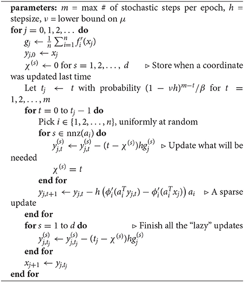
Algorithm 1 (S2GD) depends on three parameters: stepsize h, constant m limiting the number of stochastic gradients computed in a single epoch, and a ν ∈ [0, μ], where μ is the strong convexity constant of f. In practice, ν would be a known lower bound on μ. Note that the algorithm works also without any knowledge of the strong convexity parameter—the case of ν = 0.
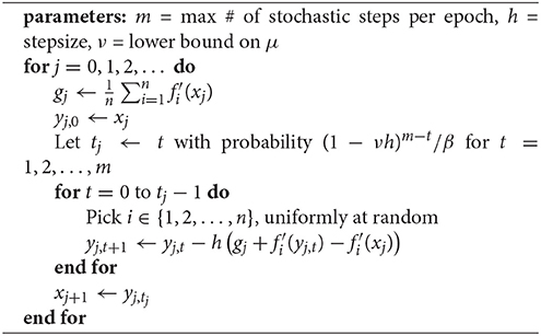
Algorithm 1. Semi-Stochastic Gradient Descent (S2GD)
The method has an outer loop, indexed by epoch counter j, and an inner loop, indexed by t. In each epoch j, the method first computes gj—the full gradient of f at xj. Subsequently, the method produces a random number tj ∈ [1, m] of steps, following a geometric law, where
with only two stochastic gradients computed in each step4. For each t = 0, …, tj − 1, the stochastic gradient is subtracted from gj, and is added to gj, which ensures that, one has
where the expectation is with respect to the random variable i.
Hence, the algorithm is stochastic gradient descent—albeit executed in a nonstandard way (compared to the traditional implementation described in the introduction).
Note that for all j, the expected number of iterations of the inner loop, E(tj), is equal to
Also note that , with the lower bound attained for ν = 0, and the upper bound for νh → 1.
2.2. S2GD+
We also implement Algorithm 2, which we call S2GD+. In our experiments, the performance of this method is superior to all methods we tested, including S2GD. However, we do not analyze the complexity of this method and leave this as an open problem.
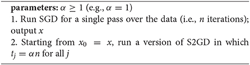
Algorithm 2. S2GD+
In brief, S2GD+ starts by running SGD for 1 epoch (1 pass over the data) and then switches to a variant of S2GD in which the number of the inner iterations, tj, is not random, but fixed to be n or a small multiple of n.
The motivation for this method is the following. It is common knowledge that SGD is able to progress much more in one pass over the data than GD (where this would correspond to a single gradient step). However, the very first step of S2GD is the computation of the full gradient of f. Hence, by starting with a single pass over data using SGD and then switching to S2GD, we obtain a superior method in practice5.
3. Summary of Results
In this section we summarize some of the main results and contributions of this work.
1. Complexity for strongly convex f. If f is strongly convex, S2GD needs
work (measured as the total number of evaluations of the stochastic gradient, accounting for the full gradient evaluations as well) to output an ε-approximate solution (in expectation or in high probability), where κ = L/μ is the condition number. This is achieved by running S2GD with stepsize h = O(1/L), j = O(log(1/ε)) epochs (this is also equal to the number of full gradient evaluations) and m = O(κ) (this is also roughly equal to the number of stochastic gradient evaluations in a single epoch). The complexity results are stated in detail in Sections 4 and 5 (see Theorems 4, 5 and 6; see also Equations 26 and 27).
2. Comparison with existing results. This complexity result (Equation 6) matches the best-known results obtained for strongly convex losses in recent work such as Roux et al. [4], Johnson and Zhang [7], and Zhang and Mahdavi [14]. Our treatment is most closely related to Johnson and Zhang [7], and contains their method (SVRG) as a special case. In Table 1 we summarize our results in the strongly convex case with other existing results for different algorithms.
We should note that the rate of convergence of Nesterov's algorithm [21] is a deterministic result. EMGD and S2GD results hold with high probability (see Theorem 5 for precise statement). Complexity results for stochastic coordinate descent methods are also typically analyzed in the high probability regime [3]. The remaining results hold in expectation. Notion of κ is slightly different for SDCA, which requires explicit knowledge of the strong convexity parameter μ to run the algorithm. In contrast, other methods do not algorithmically depend on this, and thus their convergence rate can adapt to any additional strong convexity locally.
3. Complexity for convex f. If f is not strongly convex, then we propose that S2GD be applied to a perturbed version of the problem, with strong convexity constant μ = O(L/ε). An ε-accurate solution of the original problem is recovered with arbitrarily high probability (see Theorem 8 in Section 6). The total work in this case is
that is, Õ(1/ϵ), which is better than the standard rate of SGD.
4. Optimal parameters. We derive formulas for optimal parameters of the method which (approximately) minimize the total workload, measured in the number of stochastic gradients computed (counting a single full gradient evaluation as n evaluations of the stochastic gradient). In particular, we show that the method should be run for O(log(1/ε)) epochs, with stepsize h = O(1/L) and m = O(κ). No such results were derived for SVRG in Johnson and Zhang [7].
5. One epoch. Consider the case when S2GD is run for 1 epoch only, effectively limiting the number of full gradient evaluations to 1, while choosing a target accuracy ϵ. We show that S2GD with ν = μ needs
work only (see Table 2). This compares favorably with the optimal complexity in the ν = 0 case (which reduces to SVRG), where the work needed is
For two epochs one could just say that we need decrease in each epoch, thus having complexity of . This is already better than general rate of SGD (O(1/ε)).
6. Special cases. GD and SVRG arise as special cases of S2GD, for m = 1 and ν = 0, respectively6.
7. Low memory requirements. Note that SDCA and SAG, unlike SVRG and S2GD, need to store all gradients (or dual variables) throughout the iterative process. While this may not be a problem for a modest sized optimization task, this requirement makes such methods less suitable for problems with very large n.
8. S2GD+. We propose a “boosted” version of S2GD, called S2GD+, which we do not analyze. In our experiments, however, it performs vastly superior to all other methods we tested, including GD, SGD, SAG and S2GD. S2GD alone is better than both GD and SGD if a highly accurate solution is required. The performance of S2GD and SAG is roughly comparable, even though in our experiments S2GD turned to have an edge.
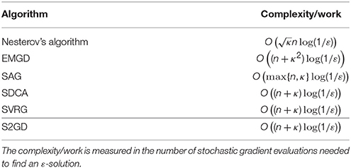
Table 1. Comparison of performance of selected methods suitable for solving Equation (1).
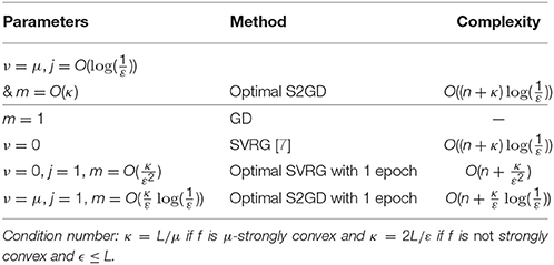
Table 2. Summary of complexity results and special cases.
4. Complexity Analysis: Strongly Convex Loss
For the purpose of the analysis, let
be the σ-algebra generated by the relevant history of S2GD. We first isolate an auxiliary result.
Lemma 3. Consider the S2GD algorithm. For any fixed epoch number j, the following identity holds:
Proof. By the tower law of conditional expectations and the definition of xj+1 in the algorithm, we obtain
□
We now state and prove the main result of this section.
Theorem 4. Let Assumptions 1 and 2 be satisfied. Consider the S2GD algorithm applied to solving problem (1). Choose 0 ≤ ν ≤ μ, , and let m be sufficiently large so that
Then we have the following convergence in expectation:
Before we proceed to proving the theorem, note that in the special case with ν = 0, we recover the result of Johnson and Zhang [7] (with a minor improvement in the second term of c where L is replaced by L − μ), namely
If we set ν = μ, then c can be written in the form (see Equation 4)
Clearly, the latter c is a major improvement on the former one. We shall elaborate on this further later.
Proof. It is well-known [21, Theorem 2.1.5] that since the functions fi are L-smooth, they necessarily satisfy the following inequality:
By summing these inequalities for i = 1, …, n, and using we get
Let be the direction of update at jth iteration in the outer loop and tth iteration in the inner loop. Taking expectation with respect to i, conditioned on the σ-algebra Equation (7), we obtain7
Above we have used the bound ||x′ + x″||2 ≤ 2||x′||2 + 2||x″||2 and the fact that
We now study the expected distance to the optimal solution (a standard approach in the analysis of gradient methods):
By rearranging the terms in Equation (16) and taking expectation over the σ-algebra , we get the following inequality:
Finally, we can analyze what happens after one iteration of the outer loop of S2GD, i.e., between two computations of the full gradient. By summing up inequalities Equation (17) for t = 1, …, m, with inequality t multiplied by (1 − νh)m−t, we get the left-hand side
and the right-hand side
Since LHS ≤ RHS, we finally conclude with
□
Since we have established linear convergence of expected values, a high probability result can be obtained in a straightforward way using Markov inequality.
Theorem 5. Consider the setting of Theorem 4. Then, for any 0 < ρ <1, 0 < ε <1 and
we have
Proof. This follows directly from Markov inequality and Theorem 4:
□
This result will be also useful when treating the non-strongly convex case.
5. Optimal Choice of Parameters
The goal of this section is to provide insight into the choice of parameters of S2GD; that is, the number of epochs (equivalently, full gradient evaluations) j, the maximal number of steps in each epoch m, and the stepsize h. The remaining parameters (L, μ, n) are inherent in the problem and we will hence treat them in this section as given.
In particular, ideally we wish to find parameters j, m and h solving the following optimization problem:
subject to
Note that is the expected work, measured by the number number of stochastic gradient evaluations, performed by S2GD when running for j epochs. Indeed, the evaluation of gj is equivalent to n stochastic gradient evaluations, and each epoch further computes on average 2ξ(m, h) stochastic gradients (see Equation 5). Since , we can simplify and solve the problem with ξ set to the conservative upper estimate ξ = m.
In view of Equation (10), accuracy constraint Equation (21) is satisfied if c (which depends on h and m) and j satisfy
We therefore instead consider the parameter fine-tuning problem:
In the following we (approximately) solve this problem in two steps. First, we fix j and find (nearly) optimal h = h(j) and m = m(j). The problem reduces to minimizing m subject to c ≤ ε1/j by fine-tuning h. While in the ν = 0 case it is possible to obtain closed form solution, this is not possible for ν > μ.
However, it is still possible to obtain a good formula for h(j) leading to expression for good m(j) which depends on ε in the correct way. We then plug the formula for m(j) obtained this way back into Equation (23), and study the quantity as a function of j, over which we optimize optimize at the end.
Theorem 6 (Choice of parameters). Fix the number of epochs j ≥ 1, error tolerance 0 < ε < 1, and let Δ = ε1/j. If we run S2GD with the stepsize
and
then E(f(xj) − f(x*)) ≤ ε(f(x0) − f(x*)).
In particular, if we choose j* = ⌈ log (1/ε)⌉, then , and hence m(j*) = O(κ), leading to the workload
Proof. We only need to show that c ≤ Δ, where c is given by Equation (12) for ν = μ and by Equation (11) for ν = 0. We denote the two summands in expressions for c as c1 and c2. We choose the h and m so that both c1 and c2 are smaller than Δ/2, resulting in c1+c2 = c ≤ Δ.
The stepsize h is chosen so that
and hence it only remains to verify that . In the ν = 0 case, m(j) is chosen so that . In the ν = μ case, holds for , where . We only need to observe that c decreases as m increases, and apply the inequality .
□
We now comment on the above result:
1. Workload. Notice that for the choice of parameters j*, h = h(j*), m = m(j*) and any ν ∈ [0, μ], the method needs log(1/ε) computations of the full gradient (note this is independent of κ), and O(κ log (1/ε)) computations of the stochastic gradient. This result, and special cases thereof, are summarized in Table 2.
2. Simpler formulas for m. If κ ≥ 2, we can instead of Equation (25) use the following (slightly worse but) simpler expressions for m(j), obtained from Equation (25) by using the bounds 1 ≤ κ − 1, κ − 1 ≤ κ and Δ <1 in appropriate places (e.g., , ):
3. Optimal stepsize in the ν = 0 case. Theorem 6 does not claim to have solved problem (23); the problem in general does not have a closed form solution. However, in the ν = 0 case a closed-form formula can easily be obtained:
Indeed, for fixed j, Equation (23) is equivalent to finding h that minimizes m subject to the constraint c ≤ Δ. In view of Equation (11), this is equivalent to searching for h > 0 maximizing the quadratic h → h(Δ − 2(ΔL+L − μ)h), which leads to Equation (28).
Note that both the stepsize h(j) and the resulting m(j) are slightly larger in Theorem 6 than in Equation (28). This is because in the theorem the stepsize was for simplicity chosen to satisfy , and hence is (slightly) suboptimal. Nevertheless, the dependence of m(j) on Δ is of the correct (optimal) order in both cases. That is, for ν = μ and for ν = 0.
4. Stepsize choice. In cases when one does not have a good estimate of the strong convexity constant μ to determine the stepsize via Equation (24), one may choose suboptimal stepsize that does not depend on μ and derive similar results to those above. For instance, one may choose .
In Table 3 we provide comparison of work needed for small values of j, and different values of κ and ε. Note, for instance, that for any problem with n = 109 and κ = 103, S2GD outputs a highly accurate solution (ε = 10− 6) in the amount of work equivalent to 2.12 evaluations of the full gradient of f!
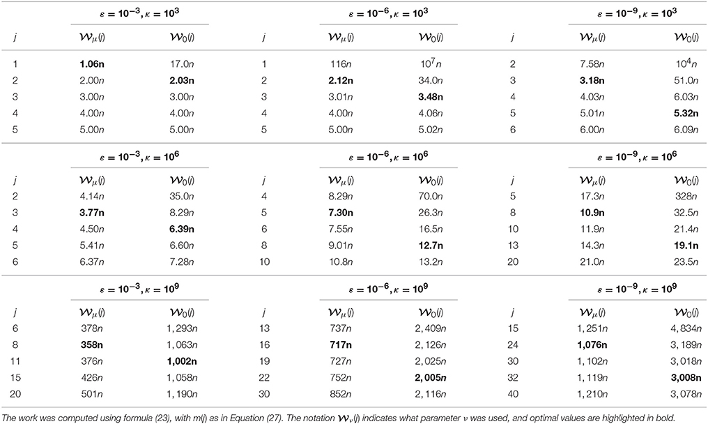
Table 3. Comparison of work sufficient to solve a problem with n = 109, and various values of κ and ε.
6. Complexity Analysis: Convex Loss
If f is convex but not strongly convex, we define , for small enough μ > 0 (we shall see below how the choice of μ affects the results), and consider the perturbed problem
where
Note that is μ-strongly convex and (L + μ)-smooth. In particular, the theory developed in the previous section applies. We propose that S2GD be instead applied to the perturbed problem, and show that an approximate solution of Equation (29) is also an approximate solution of Equation (1) (we will assume that this problem has a minimizer).
Let be the (necessarily unique) solution of the perturbed problem (29). The following result describes an important connection between the original problem and the perturbed problem.
Lemma 7. If satisfies , where δ > 0, then
Proof. The statement is almost identical to Lemma 9 in Richtárik and Takáč [3]; its proof follows the same steps with only minor adjustments. □
We are now ready to establish a complexity result for non-strongly convex losses.
Theorem 8. Let Assumption 1 be satisfied. Choose μ > 0, 0 ≤ ν ≤ μ, stepsize , and let m be sufficiently large so that
Pick and let be the sequence of iterates produced by S2GD as applied to problem (29). Then, for any 0 < ρ < 1, 0 < ε < 1 and
we have
In particular, if we choose μ = ϵ < L and parameters j*, h(j*), m(j*) as in Theorem 6, the amount of work performed by S2GD to guarantee Equation (33) is
which consists of full gradient evaluations and stochastic gradient evaluations.
Proof. We first note that
where the first inequality follows from , and the second one from optimality of x*. Hence, by first applying Lemma 7 with and δ = ε(f(x0)−f(x*)), and then Theorem 5, with c ← ĉ, , , , we obtain
The second statement follows directly from the second part of Theorem 6 and the fact that the condition number of the perturbed problem is . □
7. Implementation for Sparse Data
In our sparse implementation of Algorithm 1, described in this section and formally stated as Algorithm 3, we make the following structural assumption:
Assumption 9. The loss functions arise as the composition of a univariate smooth loss function ϕi, and an inner product with a data point/example :
In this case, .
This is the structure in many cases of interest, including linear or logistic regression.
Algorithm 3 Semi-Stochastic Gradient Descent (S2GD) for sparse data; “lazy” updates
A natural question one might want to ask is whether S2GD can be implemented efficiently for sparse data.
Let us first take a brief detour and look at SGD, which performs iterations of the type:
Let ωi be the number of nonzero features in example ai, i.e., . Assuming that the computation of the derivative of the univariate function ϕi takes O(1) amount of work, the computation of ∇fi(x) will take O(ωi) work. Hence, the update step Equation (35) will cost O(ωi), too, which means the method can naturally speed up its iterations on sparse data.
The situation is not as simple with S2GD, which for loss functions of the type described in Assumption 9 performs inner iterations as follows:
Indeed, note that is in general be fully dense even for sparse data {ai}. As a consequence, the update in Equation (36) might be as costly as d operations, irrespective of the sparsity level ωi of the active example ai. However, we can use the following “lazy/delayed” update trick. We split the update to the y vector into two parts: immediate, and delayed. Assume index i = it was chosen at inner iteration t. We immediately perform the update
which costs O(ait). Note that we have not computed the yj,t+1. However, we “know” that
without having to actually compute the difference. At the next iteration, we are supposed to perform update Equation (36) for i = it+1:
However, notice that we can't compute
as we never computed yj,t+1. However, here lies the trick: as ait+1 is sparse, we only need to know those coordinates s of yj,t+1 for which is nonzero. So, just before we compute the (sparse part of) of the update Equation (37), we perform the update
for coordinates s for which is nonzero. This way we know that the inner product appearing in Equation (38) is computed correctly (despite the fact that yj,t+1 potentially is not!). In turn, this means that we can compute the sparse part of the update in Equation (37).
We now continue as before, again only computing ỹj,t+3. However, this time we have to be more careful as it is no longer true that
We need to remember, for each coordinate s, the last iteration counter t for which . This way we will know how many times did we “forget” to apply the dense update . We do it in a just-in-time fashion, just before it is needed.
Algorithm 3 (sparse S2GD) performs these lazy updates as described above. It produces exactly the same result as Algorithm 1 (S2GD), but is much more efficient for sparse data as iteration picking example i only costs O(ωi). This is done with a memory overhead of only O(d) (as represented by vector χ ∈ ℝd).
8. Numerical Experiments
In this section we conduct computational experiments to illustrate some aspects of the performance of our algorithm. In Section 8.1 we consider the least squares problem with synthetic data to compare the practical performance and the theoretical bound on convergence in expectations. We demonstrate that for both SVRG and S2GD, the practical rate is substantially better than the theoretical one. In Section 8.2 we compare the S2GD algorithm on several real datasets with other algorithms suitable for this task. We also provide efficient implementation of the algorithm, as described in Section 7, for the case of logistic regression in the MLOSS repository8.
8.1. Comparison with Theory
Figure 1 presents a comparison of the theoretical rate and practical performance on a larger problem with artificial data, with a condition number we can control (and choose it to be poor). In particular, we consider the L2-regularized least squares with
for some , bi ∈ ℝ and λ > 0 is the regularization parameter.
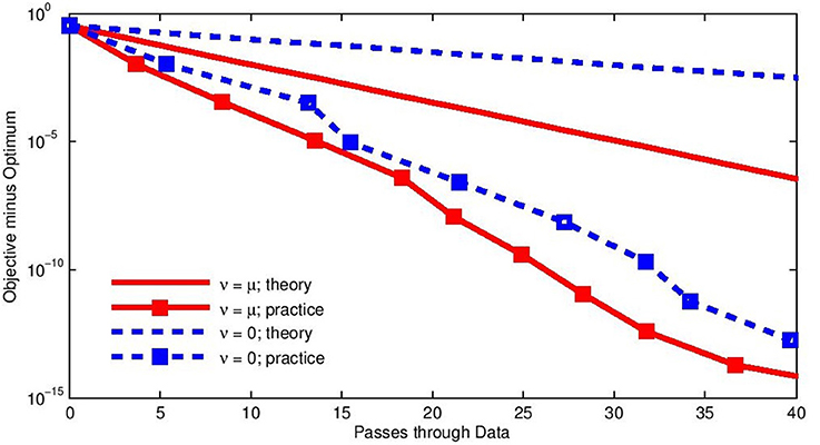
Figure 1. Least squares with n = 105, κ = 104. Comparison of theoretical result and practical performance for cases ν = μ (full red line) and ν = 0 (dashed blue line).
We consider an instance with n = 100, 000, d = 1, 000 and κ = 10, 000. We run the algorithm with both parameters ν = λ (our best estimate of μ) and ν = 0. Recall that the latter choice leads to the SVRG method of [7]. We chose parameters m and h as a (numerical) solution of the work-minimization problem (20), obtaining m = 261, 063 and h = 1/11.4L for ν = λ and m = 426, 660 and h = 1/12.7L for ν = 0. The practical performance is obtained after a single run of the S2GD algorithm.
The figure demonstrates linear convergence of S2GD in practice, with the convergence rate being significantly better than the already strong theoretical result. Recall that the bound is on the expected function values. We can observe a rather strong convergence to machine precision in work equivalent to evaluating the full gradient only 40 times. Needless to say, neither SGD nor GD have such speed. Our method is also an improvement over [7], both in theory and practice.
8.2. Comparison with other Methods
The S2GD algorithm can be applied to several classes of problems. We perform experiments on an important and in many applications used L2-regularized logistic regression for binary classification on several datasets. The functions fi in this case are:
where li is the label of ith training exapmle ai. In our experiments we set the regularization parameter λ = O(1/n) so that the condition number κ = O(n), which is about the most ill-conditioned problem used in practice. We added a (regularized) bias term to all datasets.
All the datasets we used, listed in Table 4, are freely available9 benchmark binary classification datasets.
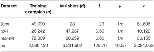
Table 4. Datasets used in the experiments.
In the experiment, we compared the following algorithms:
• SGD: Stochastic Gradient Descent. After various experiments, we decided to use a variant with constant step-size that gave the best practical performance in hindsight.
• L-BFGS: A publicly-available limited-memory quasi-Newton method that is suitable for broader classes of problems. We used a popular implementation by Mark Schmidt10.
• SAG: Stochastic Average Gradient, Schmidt et al. [5]. This is the most important method to compare to, as it also achieves linear convergence using only stochastic gradient evaluations. Although the methods has been analyzed for stepsize h = 1/16L, we experimented with various stepsizes and chose the one that gave the best performance for each problem individually.
• SDCA: Stochastic Dual Coordinate Ascent, where we used approximate solution to the one-dimensional dual step, as in Section 6.2 of Shalev-Shwartz and Zhang [6].
• S2GDcon: The S2GD algorithm with conservative stepsize choice, i.e., following the theory. We set m = O(κ) and h = 1/10L, which is approximately the value you would get from Equation (24).
• S2GD: The S2GD algorithm, with stepsize that gave the best performance in hindsight. The best value of m was between n and 2n in all cases, but optimal h varied from 1/2L to 1/10L.
Note that SAG needs to store n gradients in memory in order to run. In case of relatively simple functions, one can store only n scalars, as the gradient of fi is always a multiple of ai. If we are comparing with SAG, we are implicitly assuming that our memory limitations allow us to do so. Although not included in Algorithm (1), we could also store these gradients we used to compute the full gradient, which would mean we would only have to compute a single stochastic gradient per inner iteration (instead of two).
We plot the results of these methods, as applied to various different, in the Figure 2 for first 15–30 passes through the data (i.e., amount of work work equivalent to 15–30 full gradient evaluations).
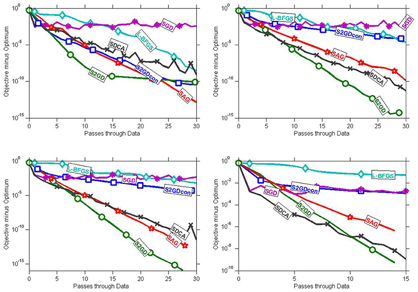
Figure 2. Practical performance for logistic regression and the following datasets: ijcnn, rcv (first row), realsim, url (second row).
There are several remarks we would like to make. First, our experiments confirm the insight from Schmidt et al. [5] that for this types of problems, reduced-variance methods consistently exhibit substantially better performance than the popular L-BFGS algorithm.
The performance gap between S2GDcon and S2GD differs from dataset to dataset. A possible explanation for this can be found in an extension of SVRG to proximal setting Xiao and Zhang [22], released after the first version of this paper was put onto arXiv (i.e., after December 2013). Instead Assumption 1, where all loss functions are assumed to be associated with the same constant L, the authors of Xiao and Zhang [22] instead assume that each loss function fi has its own constant Li. Subsequently, they sample proportionally to these quantities as opposed to the uniform sampling. In our case, . This weighted sampling has an impact on the convergence: one gets dependence on the average of the quantities Li and not in their maximum.
The number of passes through data seems a reasonable way to compare performance, but some algorithms could need more time to do the same amount of passes through data than others. In this sense, S2GD should be in fact faster than SAG due to the following property. While SAG updates the test point after each evaluation of a stochastic gradient, S2GD does not always make the update—during the evaluation of the full gradient. This claim is supported by computational evidence: SAG needed about 20–40% more time than S2GD to do the same amount of passes through data.
Finally, in Table 5 we provide the time it took the algorithm to produce these plots on a desktop computer with Intel Core i7 3610QM processor, with 2 × 4 GB DDR3 1,600 MHz memory. The numbers for the url dataset is are not representative, as the algorithm needed extra memory, which slightly exceeded the memory limit of our computer.
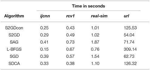
Table 5. Time required to produce plots in Figure 2.
8.3. Boosted variants of S2GD and SAG
In this section we study the practical performance of boosted methods, namely S2GD+ (Algorithm 2) and variant of SAG suggested by its authors [5, Section 4.2].
SAG+ is a simple modification of SAG, where one does not divide the sum of the stochastic gradients by n, but by the number of training examples seen during the run of the algorithm, which has the effect of producing larger steps at the beginning. The authors claim that this method performed better in practice than a hybrid SG/SAG algorithm.
We have observed that, in practice, starting SAG from a point close to the optimum, leads to an initial “away jump.” Eventually, the method exhibits linear convergence. In contrast, S2GD converges linearly from the start, regardless of the starting position.
Figure 3 shows that S2GD+ consistently improves over S2GD, while SAG+ does not improve always: sometimes it performs essentially the same as SAG. Although S2GD+ is overall a superior algorithm, one should note that this comes at the cost of having to choose stepsize parameter for SGD initialization. If one chooses these parameters poorly, then S2GD+ could perform worse than S2GD. The other three algorithms can work well without any parameter tuning.
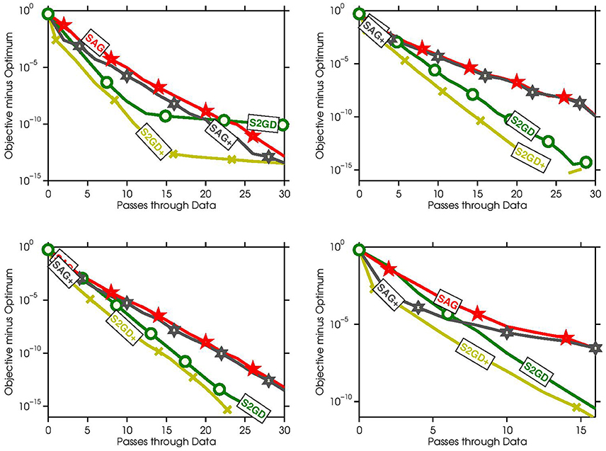
Figure 3. Practical performance of boosted methods on datasets ijcnn, rcv (first row), realsim, url (second row).
9. Conclusion
We have developed a new semi-stochastic gradient descent method (S2GD) and analyzed its complexity for smooth convex and strongly convex loss functions. Our methods need O((κ/n) log(1/ε)) work only, measured in units equivalent to the evaluation of the full gradient of the loss function, where κ = L/μ if the loss is L-smooth and μ-strongly convex, and κ ≤ 2L/ε if the loss is merely L-smooth.
Our results in the strongly convex case match or improve on a few very recent results, while at the same time generalizing and simplifying the analysis. Additionally, we proposed S2GD+—a method which equips S2GD with an SGD pre-processing step—which in our experiments exhibits superior performance to all methods we tested. We leave the analysis of this method as an open problem.
Author Contributions
All authors listed, have made substantial, direct and intellectual contribution to the work, and approved it for publication.
Funding
The work of both authors was supported by the Centre for Numerical Algorithms and Intelligent Software (funded by EPSRC grant EP/G036136/1 and the Scottish Funding Council). Both authors also thank the Simons Institute for the Theory of Computing, UC Berkeley, where this work was conceived and finalized. The work of PR was also supported by the EPSRC grant EP/I017127/1 (Mathematics for Vast Digital Resources) and EPSRC grant EP/K02325X/1 (Accelerated Coordinate Descent Methods for Big Data Problems).
Conflict of Interest Statement
The authors declare that the research was conducted in the absence of any commercial or financial relationships that could be construed as a potential conflict of interest.
Footnotes
1. ^The question of whether or when primal or dual version is better has recently been studied in Csiba and Richtárik [8] to which we refer the reader for further details.
2. ^We thank Zaid Harchaoui who pointed us to these papers a few days before we posted our work to arXiv.
3. ^Since the first version of our work, our proposed algorithm has been extended to apply to a more broader class functions in Konečný et al. [20].
4. ^It is possible to get away with computing only a single stochastic gradient per inner iteration, namely , at the cost of having to store in memory for i = 1, 2, …, n. This, however, can be impractical for big n.
5. ^Using a single pass of SGD as an initialization strategy was already considered in Roux et al. [4]. However, the authors claim that their implementation of vanilla SAG did not benefit from it. S2GD does benefit from such an initialization due to it starting, in theory, with a (heavy) full gradient computation.
6. ^While S2GD reduces to GD for m = 1, our analysis does not say anything meaningful in the m = 1 case—it is too coarse to cover this case. This is also the reason behind the empty space in the “Complexity” box column for GD in Table 2.
7. ^For simplicity, we supress the notation here.
8. ^http://mloss.org/software/view/556/
9. ^Available at http://www.csie.ntu.edu.tw/~cjlin/libsvmtools/datasets/.
References
1. Nemirovski A, Juditsky A, Lan G, Shapiro A. Robust stochastic approximation approach to stochastic programming. SIAM J Optim. (2009) 19:1574–609. doi: 10.1137/070704277
2. Zhang T. Solving large scale linear prediction problems using stochastic gradient descent algorithms. In: The International Conference on Machine Learning. Banff, AB (2004).
3. Richtárik P, Takáč M. Iteration complexity of randomized block-coordinate descent methods for minimizing a composite function. Math Progr. (2014) 144:1–38. doi: 10.1007/s10107-012-0614-z
4. Roux NL, Schmidt M, Bach FR. A stochastic gradient method with an exponential convergence _rate for finite training sets. In: Advances in Neural Information Processing Systems. Lake Tahoe (2012) p. 2663–71.
5. Schmidt M, Le Roux N, Bach F. Minimizing finite sums with the stochastic average gradient. Math Progr. (2017) 162:83–112. doi: 10.1007/s10107-016-1030-6
6. Shalev-Shwartz S, Zhang T. Stochastic dual coordinate ascent methods for regularized loss minimization. J Mach Learn Res. (2013) 14:567–99. Available online at: http://www.jmlr.org/papers/v14/shalev-shwartz13a.html
7. Johnson R, Zhang T. Accelerating stochastic gradient descent using predictive variance reduction. In: Advances in Neural Information Processing Systems. Lake Tahoe (2013).
8. Csiba D, Richtárik P. Coordinate descent face-off: primal or dual? arXiv preprint arXiv:160508982 (2016).
9. Hsieh CJ, Chang KW, Lin CJ, Keerthi SS, Sundarajan S. A dual coordinate descent method for large-scale linear SVM. In: International Conference on Machine Learning. Helsinki (2008). doi: 10.1145/1390156.1390208
10. Takáč M, Bijral A, Richtárik P, Srebro N. Mini-batch primal and dual methods for SVMs. In: International Conference on Machine Learning (2013).
11. Richtárik P, Takáč M. Parallel coordinate descent methods for big data optimization. Math Progr. (2016) 156:433–84. doi: 10.1007/s10107-015-0901-6
12. Fercoq O, Richtárik P. Smooth minimization of nonsmooth functions with parallel coordinate descent methods. arXiv:13095885 (2013).
13. Richtárik P, Takáč M. Distributed coordinate descent method for learning with big data. J Mach Learn Res. (2016) 17:1–25. Available online at: http://www.jmlr.org/papers/v17/15-001.html
14. Zhang L, Mahdavi M, Jin R. Linear convergence with condition number independent access of full gradients. In: Advances in Neural Information Processing Systems. Lake Tahoe (2013).
15. Friedlander MP, Schmidt M. Hybrid deterministic-stochastic methods for data fitting. SIAM J Sci Comput. (2012) 34:A1380–405. doi: 10.1137/110830629
16. Deng G, Ferris MC. Variable-number sample-path optimization. Math Progr. (2009) 117:81–109. doi: 10.1007/s10107-007-0164-y
17. Bastin F, Cirillo C, Toint PL. Convergence theory for nonconvex stochastic programming with an application to mixed logit. Math Progr. (2006) 108:207–34. doi: 10.1007/s10107-006-0708-6
18. Marti K, Fuchs E. On solutions of stochastic programming problems by descent procedures with stochastic and deterministic directions. Methods Operat Res. (1979) 33:281–93.
19. Marti K, Fuchs E. Rates of convergence of semi-stochastic approximation procedures for solving stochastic optimization problems. Optimization (1986) 17:243–65. doi: 10.1080/02331938608843124
20. Konečný J, Liu J, Richtárik P, Takáč M. Mini-batch semi-stochastic gradient descent in the proximal setting. IEEE J Select Top Signal Process. (2016) 10:242–55. doi: 10.1109/JSTSP.2015.2505682
21. Nesterov Y. Introductory Lectures on Convex Optimization: A Basic Course. Vol. 87. Springer (2004).
Keywords: stochastic gradient, variance reduction, empirical risk minimization, linear convergence, convex optimization
Citation: Konečný J and Richtárik P (2017) Semi-Stochastic Gradient Descent Methods. Front. Appl. Math. Stat. 3:9. doi: 10.3389/fams.2017.00009
Received: 24 October 2016; Accepted: 08 May 2017;
Published: 23 May 2017.
Edited by:
Darinka Dentcheva, Stevens Institute of Technology, United StatesReviewed by:
Yu Du, Rutgers University, United StatesVladimir Shikhman, Technische Universität Chemnitz, Germany
Uday V. Shanbhag, Pennsylvania State University, United States
Copyright © 2017 Konečný and Richtárik. This is an open-access article distributed under the terms of the Creative Commons Attribution License (CC BY). The use, distribution or reproduction in other forums is permitted, provided the original author(s) or licensor are credited and that the original publication in this journal is cited, in accordance with accepted academic practice. No use, distribution or reproduction is permitted which does not comply with these terms.
*Correspondence: Jakub Konečný, kubo.konecny@gmail.com