1
Program in Neurosciences and Mental Health, The Hospital for Sick Children, Toronto, ON, Canada
2
Department of Physiology, University of Toronto, Toronto, ON, Canada
3
Institute of Medical Science, University of Toronto, Toronto, ON, Canada
In the water maze, mice are trained to navigate to an escape platform located below the water’s surface, and spatial learning is most commonly evaluated in a probe test in which the platform is removed from the pool. While contemporary tracking software provides precise positional information of mice for the duration of the probe test, existing performance measures (e.g., percent quadrant time, platform crossings) fail to exploit fully the richness of this positional data. Using the concept of entropy (H), here we develop a new measure that considers both how focused the search is and the degree to which searching is centered on the former platform location. To evaluate how H performs compared to existing measures of water maze performance we compiled five separate databases, containing more than 1600 mouse probe tests. Random selection of individual trials from respective databases then allowed us to simulate experiments with varying sample and effect sizes. Using this Monte Carlo-based method, we found that H outperformed existing measures in its ability to detect group differences over a range of sample or effect sizes. Additionally, we validated the new measure using three models of experimentally induced hippocampal dysfunction: (1) complete hippocampal lesions, (2) genetic deletion of αCaMKII, a gene implicated in hippocampal behavioral and synaptic plasticity, and (3) a mouse model of Alzheimer’s disease. Together, these data indicate that H offers greater sensitivity than existing measures, most likely because it exploits the richness of the precise positional information of the mouse throughout the probe test.
A fundamental goal in neuroscience is to understand how genes (or networks of genes) contribute to learning and memory. In this regard, one key advance has been the development of molecular genetic tools that allow the expression of individual genes to be manipulated in a spatially and temporally specific manner. Perhaps less appreciated, however, is the importance of developing behavioral assays that can detect learning phenotypes with greater sensitivity (Tecott and Nestler, 2004
).
Presently, a wide variety of tasks may be used to assess learning and memory in mice (Crawley, 2008
). For forms of learning that depend primarily upon the hippocampus, the water maze is perhaps the most pervasive (Morris, 1981
, 1984
; Morris et al., 1982
). In this task, mice are placed in a circular tank filled with opaque water and learn to escape from the water by navigating to a platform submerged below the water’s surface. Typically, over the course of training, mice learn to search more focally and, as a result, their escape latencies decline. The shift toward more focal searching is most commonly evaluated by measuring where mice search in a probe test where the escape platform is removed from the pool (Morris, 1984
; Wolfer et al., 2001
; Clapcote and Roder, 2004
; Vorhees and Williams, 2006
; Kee et al., 2007a
).
Tracking software provides precise positional information of mice for the duration of the probe test. While existing measures of probe test performance – such as the percent time spent in a virtual quadrant or zone centered on the former platform location – may readily distinguish different treatment groups, they fail to exploit fully the richness of this positional data. This leaves open the possibility that measures that more fully exploit this richness may offer greater sensitivity in detecting learning phenotypes.
Accordingly, here we use the concept of entropy (H) – a measure of the disorder of a system – to develop a new water maze performance metric. Entropy provides a potentially useful framework, since the shift toward more focal searching that might occur over the course of learning can be considered as a transition from a high (or disordered) to a low (or ordered) state of entropy. In order to evaluate how our new H measure compares with existing measures, we conducted a series of Monte Carlo simulations using five separate databases containing more than 1600 probe tests. These analyses revealed that H outperforms existing measures over a range of sample or effect sizes, and using both parametric and non-parametric statistical tests. Finally, we validated H using three models of experimentally induced hippocampal dysfunction [complete hippocampal lesions (Logue et al., 1997
; Cho et al., 1999
), a mouse model of Alzheimer’s disease (Janus et al., 2000
), and a genetic deletion of αCaMKII (Elgersma et al., 2002
)].
Derivation of New Entropy (H) Measure
Here we use the concept of entropy – a measure of the disorder of a system – to quantify water maze probe test performance. Over the course of training mice typically learn to search more focally (i.e., searching that is centered on the former platform location with little variance). This shift in search strategy can then be considered as a transition from a high (or disordered) to a low (or ordered) state of entropy. Therefore, we can start from the definition of entropy. In the context of information theory, entropy describes the uncertainty associated with a random variable. For a continuous one-dimensional random variable x with probability density function p(x), its information entropy H is:

If X follows a normal distribution, it can be shown that:

Because 1/2 ln(2πe) is a constant, it can be dropped to further simplify the measure as:

It can be further shown that if X is a two-dimensional variable, then

where σa and σb are the radii of each major axis of the error ellipse. For a detailed derivation, please see Li et al. (2003
).
For any given search, we can consider two types of entropy: First, error entropy (or the variance of the mouse’s position with respect to the target, Herror); Second, path entropy (or the variance of the mouse’s position with respect to the focus of its path; Hpath). Because each of these components is computed over 2-D space, where the x and y coordinates of each point are random variables, we can use Eq. 4 to describe them. Accordingly, error variance or Herror (Figure 1
A) may be represented by:
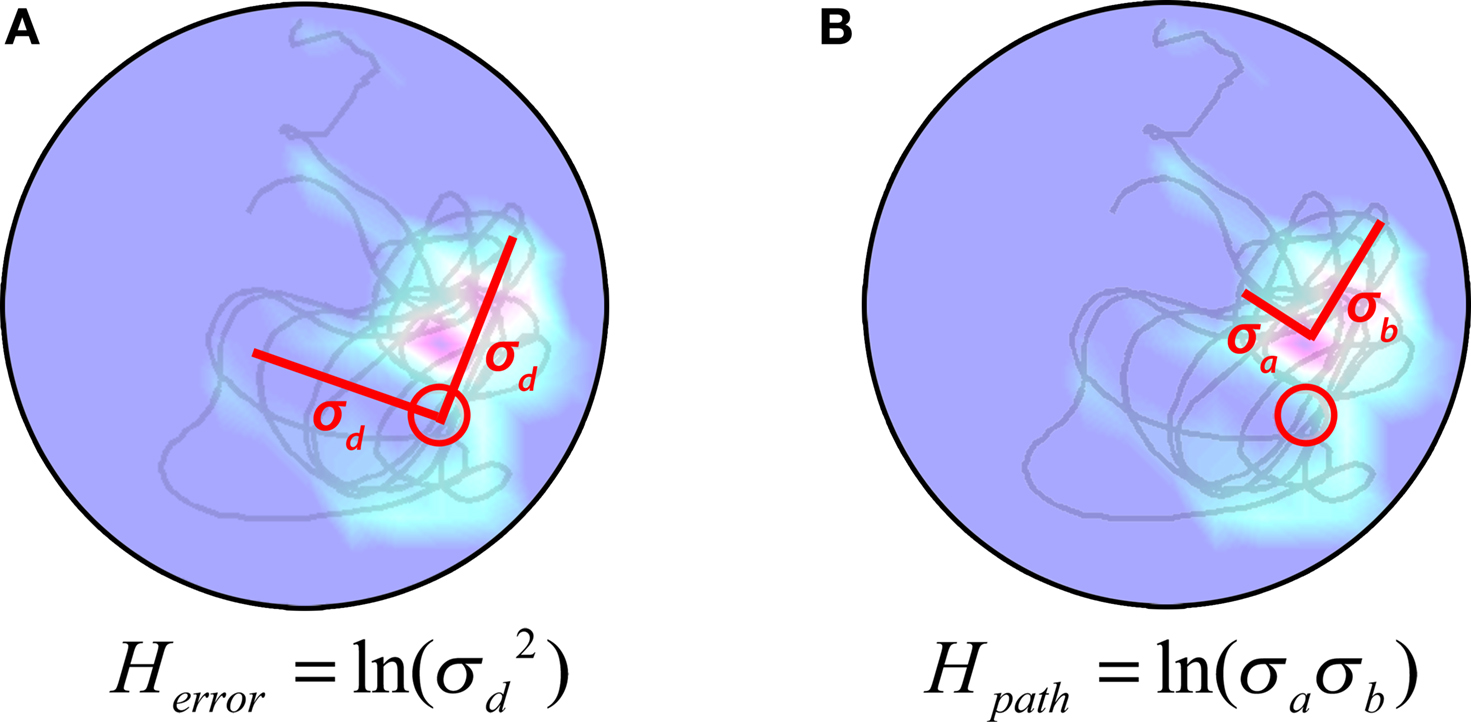
Figure 1. The H measure. (A) The Herror component, centered on platform location and varying in two dimensions by σd and σd. (B) The Hpath component, centered on the mean location of the animal’s trajectory and varying in two dimensions by σa and σb.
Because in the case of Herror, we are concerned with the distance of each point from the platform, we can simplify the expression and the corresponding ellipse to a circle by calculating the distance of each point from the platform given the two coordinates:

Similarly, path variance or Hpath (Figure 1
B) may be represented by:

Because entropy is additive (Li et al., 2003
), the total entropy of the search is then the sum of the two equations:

where the first term is the entropy of the error and the second term is the entropy of the path.
Data Sets and Behavioral Procedures
Probe test data were pooled from experiments conducted in the laboratory between June 2004 and June 2008. All experiments were conducted using identical apparatus, training and probe test procedures, as described below.
Apparatus
Water maze experiments were conducted in a circular tank (120 cm in diameter, 50 cm deep), located in a dimly-lit room (Teixeira et al., 2006
; Kee et al., 2007a
,b
; Wang et al., 2009
). The pool was filled to a depth of 40 cm with water made opaque by adding white non-toxic paint. Water temperature was maintained at 28 ± 1°C by a heating pad located beneath the pool. A circular escape platform (5 cm radius) was submerged 0.5 cm below the water surface and located in the south-east quadrant. The pool was surrounded by curtains, at least 1 m from the perimeter of the pool. The curtains were white, and had distinct cues painted on them.
Training procedures
Prior to the commencement of training, mice were individually handled for 2 min each day for 1 week. On each training day, mice received six training trials (presented in two blocks of three trials; inter-block interval of ∼1 h, inter-trial interval was ∼15 s). On each trial they were placed into the pool, facing the wall, in one of four start locations (north, south, east, west). The order of these start locations was pseudo-randomly varied throughout training. The trial was complete once the mouse found the platform or 60 s had elapsed. If the mouse failed to find the platform on a given trial, the experimenter guided the mouse onto the platform.
Probe test procedures
During the probe test, mice were placed into the pool facing the wall, in the north location. The probe test was 60 s in duration.
Quantification of probe test performance
Behavioral data from the probe tests were acquired and analyzed using an automated tracking system (Actimetrics, Wilmette, IL, USA). Using this software, the precise mouse location (in x, y coordinates) was recorded throughout the probe test (capture rate 10 frames/s). In addition to computing the new entropy-based measure, the following existing measures of probe test performance were computed:
1) Percent quadrant time (Q). Amount of time mice searched virtual quadrant (i.e., 25% of total pool surface area), centered on the location of the platform during training (Morris, 1981
, 1984
; Morris et al., 1982
).
2) Percent zone (Z). Amount of time mice searched a virtual target zone 20 cm in radius, centered on the location of the platform during training during the 60 s test (Moser et al., 1993
; Moser and Moser, 1998
; de Hoz et al., 2004
). This zone represents 1/9th (∼11.1%) of the total pool surface area.
3) Crossings (X). Number of times mice cross the exact location of the platform (5 cm in radius) during the 60 s test (Morris, 1981
, 1984
; Morris et al., 1982
).
4) Proximity (P) measure (Gallagher’s measure) (Gallagher et al., 1993
). Average distance in cm of mice from center of the platform location across the 60 s test.
These measures (or combinations thereof) are used to quantify probe test performance in more than 98% of published papers (Maei et al., 2009
).
Analysis A. In the first analysis, probe test data were pooled from experiments where mice were initially trained for 5 days (six trials per day) and then given a probe test at variable delays following the completion of training
1
. These experiments examined the impact of different genetic, pharmacological and neuroanatomical lesion manipulations on water maze performance (for details see Teixeira et al., 2006
; Kee et al., 2007b
; Wang et al., 2009
). For these analyses, probe test data were divided into two data sets. First, a control data set (N = 370 probe tests) that included data from control mice in the genetic [i.e., wild-type (WT) mice], pharmacological (i.e., mice received control infusions of phosphate-buffered saline) and neuroanatomical lesion (i.e., sham surgery) experiments. Second, an experimental data set (N = 388 probe tests) that included data from experimental mice in the genetic [e.g., α-CaMKIIT286A knockin mice (Giese et al., 1998
; Kee et al., 2007b
)], pharmacological [e.g., mice received lidocaine infusion into the dorsal hippocampus prior to testing (Teixeira et al., 2006
)] and neuroanatomical lesion [i.e., NMDA-induced complete hippocampal lesion (Wang et al., 2009
)] experiments
2
.
Analysis B. In the second analysis, probe test data were pooled from experiments where WT mice (N = 282) were trained for 5 days with six trials per day. At variable delays following the completion of training, they received a series of three consecutive probe tests. Performance declined across probe tests, most likely reflecting extinction of spatial memory (Lattal et al., 2003
). The decline in performance therefore provides three datasets with three distinct levels of performance (see Figure 6
A).
Quantitative and Statistical Analyses
Datasets used for Analyses A and B were exported to Matlab
3
and the new H measure, as well as Q, Z, X and P measures were computed for each individual trajectory. For each dataset, descriptive statistics (mean, standard deviation) were computed for all measures. Additionally, the Lilliefors [Kolmogorov–Smirnov (K–S)] test was used to evaluate whether H, as well as existing, measures were normally distributed (see also Maei et al., 2009
). Finally, Pearson’s r was computed to evaluate how H and existing measures were correlated.
In order to compare the sensitivity of H vs. existing measures a series of simulated experiments were conducted (see Maei et al., 2009
). For Analysis A, N (range 5–40 for each group) probe tests were randomly selected (without replacement) from the control and experimental datasets, respectively. Whether the two samples differed was then evaluated using both parametric (t-test) or non-parametric (K–S) tests. For each N, 1000 simulations were conducted and, to compute the rate of rejection of the null hypothesis, 10 replications were performed. In order to evaluate the false-positive rate, the above analyses were repeated, but both samples were drawn from the control dataset. All analyses were conducted with α set at 0.05, 0.01 and 0.005, respectively. For Analysis B, a similar series of simulations were conducted to compare the probes 1, 2 and 3 datasets.
In the H measure, error and path variance contribute equally (i.e., Htotal = Herror + Hpath). In order to assess the relative contribution of these two components to the sensitivity of the measure, we conducted an additional series of simulations for both Analyses A and B. In these simulations, for different sample sizes (range 5–25), the relative weighting of Herror(λ) and Hpath(1 − λ) was varied (range 0 → 1.0, 0.1 increments).
Validation of H Measure in Mice with Experimentally Induced Hippocampal Dysfunction
Hippocampal lesions
Male offspring from a cross between C57Bl/6NTacfBr [C57B6] and 129Svev [129] mice (Taconic, Germantown, NY, USA) were used to examine the impact of complete hippocampal lesions on water maze learning
4
. Mice were treated with atropine (5 mg/kg, ip) and anesthetized with chloral hydrate (20 mg/kg, ip), as previously described (Wang et al., 2009
). In order to prevent seizure activity associated with neurotoxic lesions, mice were additionally pretreated with diazepam (5 mg/kg, ip, Sigma, St. Louis, MO, USA). Using standard stereotaxic procedures, N-methyl-d-aspartic acid (10 mg/ml; NMDA, Sigma, St. Louis, MO, USA) was infused into the following eight sites with respect to bregma: −1.8 mm (posterior), ±1.2 mm (lateral), 2.0 mm (ventral) (volume 0.1 μl); −2.3 mm (posterior), ±1.5 mm (lateral), 2.0 mm (ventral) (volume 0.1 μl); −3.0 mm (posterior), ±2.0 mm (lateral), 2.0 mm (ventral) (volume 0.1 μl); and −3.0 mm (posterior), ±2.75 mm (lateral), 3.0 mm (ventral) (volume 0.25 μl). NMDA was delivered via a 32-guage injection needle connected to a Hamilton microsyringe (Hamilton, Reno, NV, USA). An infusion pump maintained the rate of infusion at 0.1 μl/min and the injection needle was left in place for 5 min following the completion of the infusion. For sham surgeries, mice were treated identically except no NMDA was infused. Mice were treated post-operatively with the analgesic ketoprofen (5 mg/kg, ip, Sigma, St. Louis, MO, USA) and allowed to recover for at least 1 week prior to the commencement of training.
After the completion of experiments, lesion extent was characterized using histological procedures described in detail elsewhere (Wang et al., 2009
). In particular, two inclusion criteria were used: (1) the lesion should be largely confined to the hippocampus, with minimal damage to surrounding tissue; and (2) neuronal loss in both the dorsal and ventral hippocampus should be minimally 80%.
αCaMKIIΔ mice
αCaMKIIΔ+/− mice, maintained in a C57Bl/6NTacfBr [C57B6] background, were crossed with 129Svev [129] mice (Taconic, Germantown, NY, USA). F2 homozygous offspring and WT controls used for behavioral analysis were obtained by crossing these F1 αCaMKIIΔ+/− mice (Elgersma et al., 2002
).
Tg-CRND8 mice
Tg-CRND8+/− mice were maintained in a 129Svev [129] background. To obtain F1 heterozygous and WT control mice for behavioral analysis these mice were crossed with C57Bl/6NTacfBr [C57B6] mice. Mice were 10 weeks of age at the start of training.
Behavioral protocols
Two behavioral procedures were used in these studies. First, one group of hippocampal-lesioned (N = 10) and sham-operated control (N = 9) mice were trained in the water maze for 11 days (three trials per day, with an inter-trial interval ∼15 s). Probe tests were conducted prior to training on days 1, 3, 5, 7, 9 and 11. Second, an additional group of hippocampal-lesioned mice (sham, N = 8, lesion, N = 9), as well as the αCaMKIIΔ (WT, N = 7, mutant, N = 10) and tg-CRND8 (WT, N = 9, mutant, N = 9) mice, were trained for 3 days (six trials per day) and a single probe test was given at the completion of training.
Descriptive Statistics for H Index
In order to examine the behavior of the new measure in experimental situations we compiled two datasets from probe tests conducted in our behavioral laboratory at The Hospital for Sick Children, Toronto, between 2004 and 2008. These data sets comprised probe tests from control (N = 370) and experimental (N = 388) mice. Representative probe test trajectories are illustrated in Figure 2
, along with corresponding H scores. These scores range from >15 for poor performers to <12 for the most accurate search trajectories. Overall, the control group searched more selectively compared to the experimental group, according to the H measure, as well as existing measures (Q, Z, X, P) (Figure 3
A). Consistent with the idea that, in general, the H measure behaved similarly to existing measures, H was significantly correlated with Q, Z, X and P (all P-values <0.01), with Pearson’s r ranging from 0.66 (H vs. X) to 0.97 (H vs. P) (Figure 3
B).
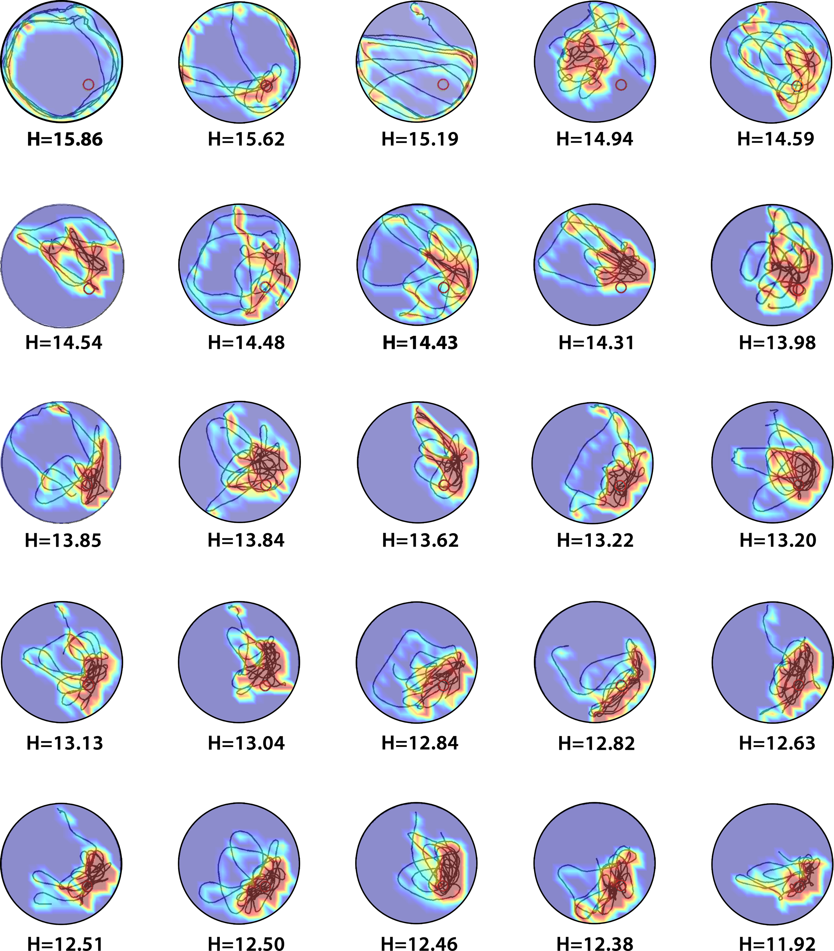
Figure 2. Sample H-scores for a range of probe test performances. The density plot generated from an individual trial is overlaid on top of the animal’s trajectory during that trial, showing where the mice concentrated their search.
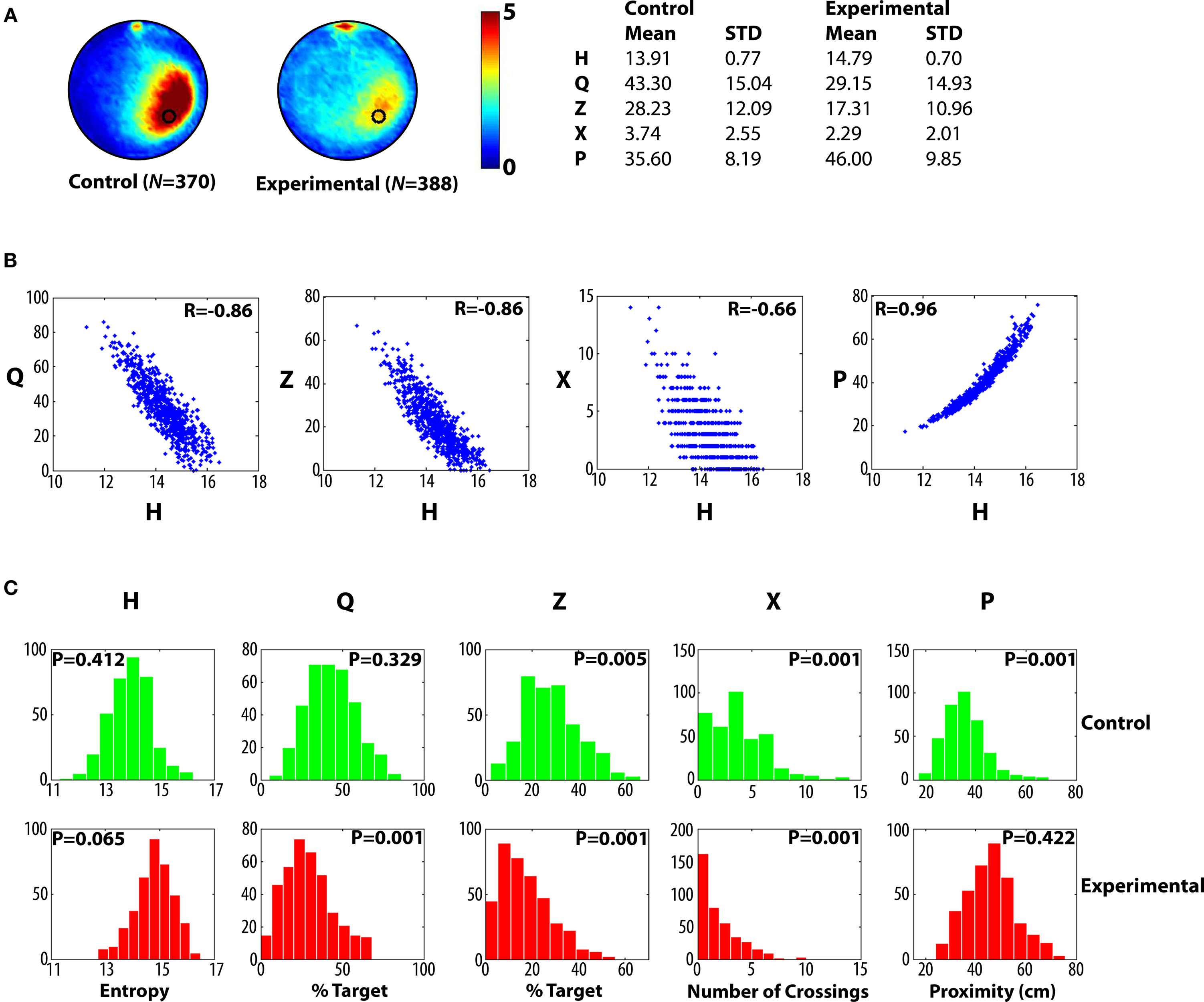
Figure 3. Pooled probe test data for control and experimental mice for Analysis A. (A) Left, density plots for grouped data showing where control and experimental mice concentrated their searches in the probe test. The color scale represents the mean number of visits per animal per 5 cm × 5 cm area. Right, summary of descriptive statistics (mean values, standard deviations) for the entropy (H), quadrant (Q), zone (Z), crossing (X) and proximity (P) measures for control and experimental datasets. (B) Scatterplots showing how H correlates with existing measures of probe test performance. (C) Distribution of probe test scores for control (upper, green) and experimental (lower, red) datasets for each measure. According to the Lilliefors adaptation of the Kolmogorov–Smirnov test, the distributions generated by the H measure are not significantly different from the normal distribution, unlike many distributions generated by the other measures, which are positively skewed (P-values <0.05).
Parametric tests (such as the Student’s t-test or ANOVA) are typically used to evaluate group differences in probe test performance. As such tests are based on the assumption that samples are drawn from populations that are normally distributed, we next evaluated the distribution of H scores in control and experimental groups. We found that H was normally distributed in both datasets (P-values >0.05; Lilliefors K–S). Notably, this is in contrast with many of the existing measures that tend to be positively skewed (Figure 3
C; see also Figure S1 in Supplementary Material; Maei et al., 2009
). Skewness was most pronounced in the experimental condition for the Q, Z and X measures, most likely because many of these mice are performing at, or near, floor levels (e.g., the majority of mice in the experimental condition fail to cross the former platform location; i.e., mode for X = 0). In such situations where the normality assumption is violated, the α set by the experimenter (e.g., 0.05) may underestimate the actual α (that is, the likelihood of a type I error or incorrectly rejecting the null hypothesis). Such effects would be most pronounced for smaller sample sizes (i.e., N-values <40) and when sample distributions are differently shaped (Sawilowsky and Hillman, 1992
).
Analysis a, Hypothesis Testing
We next conducted a series of simulated experiments to compare the sensitivity of the H index with existing measures. Experiments were simulated by randomly selecting N probe tests (without replacement) from the control and experimental groups respectively, and testing for group differences for each of the five measures using the K–S test, a non-parametric statistic that makes no assumptions about the underlying distributions of the two samples. For each N, 1000 simulations were conducted and, to compute the rate of rejection of the null hypothesis for each N, 10 replications were performed (Figure 4
A). As group size increased, the detection rates increased for all measures. For N-values up to around 40, we found that rates of rejection of the null hypothesis were consistently higher for H compared to other measures, indicating that H was more sensitive at detecting differences. For example, with α set at 0.05 and N = 15, detection rates were highest for H (∼74.4%), followed closely by P (∼72.2%) and then Z (∼52.4%), Q (∼49.5%) and X (∼14.2%). This advantage of H over P held with α set at 0.01 and 0.005 (Figure 4
A) and when t-tests, rather than K–S tests, were used to compare groups (Figure S2 in Supplementary Material).
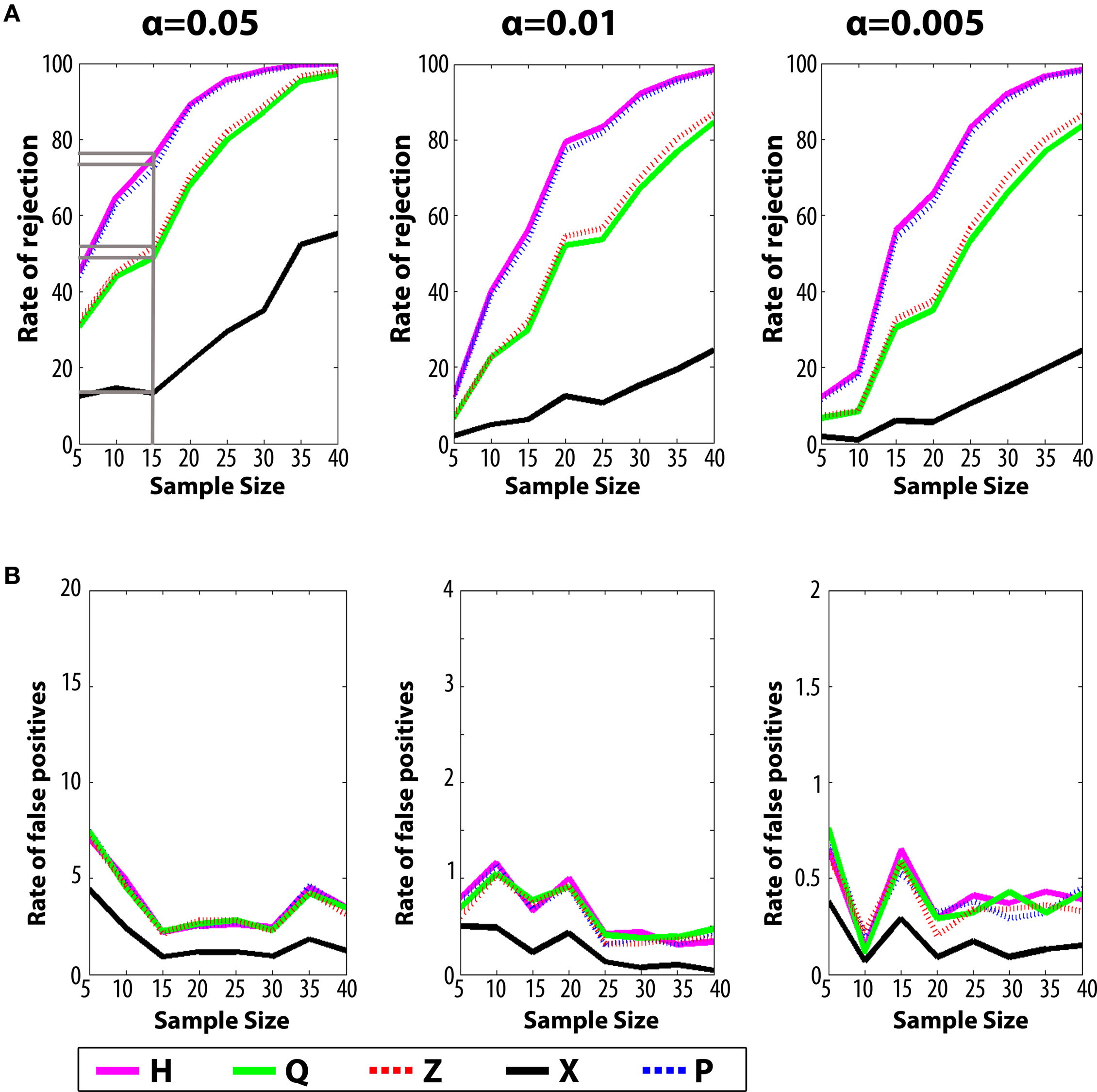
Figure 4. Monte Carlo simulations (Analysis A). (A) The likelihood of detecting a difference between control and experimental groups is shown for varying sample (N) size, with significance levels α = 0.05, 0.01 and 0.001. The non-parametric Kolmogorov–Smirnov (K–S) test was used for hypothesis testing. (B) False-positive rates when both samples are drawn from the control dataset.
With α set at 0.05 in the above simulations we would expect a false positive rate of ∼5%. To verify that false positive rates were as expected we performed the same analyses as above, but randomly selected two groups of N probe tests from the same control population (Figure 4
B) (for similar simulations using t-tests see additionally Figure S3 in Supplementary Material). For low sample sizes, false-positive rates were at expected levels for all measures when α was set at 0.05, 0.01 and 0.005, respectively.
Relative Weighting of Herror and Hpath
Two components contribute to the H measure – error (Herror) and path (Hpath) variance. In computing H, we have weighted these two variances equally (i.e., Htotal = Herror + Hpath). However, we next wondered whether the sensitivity of H would vary as a function of the relative weighting of Herror and Hpath. To address this we conducted an additional series of simulations using the control and experimental datasets. In these simulations we used sample sizes ranging from N = 5 to N = 25 (covering the range of typical sample sizes used in the majority of mouse water maze studies). In these simulations, weighting of Herror and Hpath was varied incrementally to determine conditions where detection rates were maximized (Figure 5
A). Using this approach we found that both error and path variance contribute to the sensitivity of the H measure: Rejection of the null hypothesis increased as the weighting for Herror increased, and was maximal when the Herror/Hpath weighting was set at 0.8/0.2 (for N = 5, 10, 20, 25) or 0.7/0.3 (for N = 15). The existing P measure is based on platform error. These analyses indicate that additional consideration of path variance enhances detection of group differences. The relative advantage of H over existing measures for different weightings and sample sizes is shown in Figure 5
B.
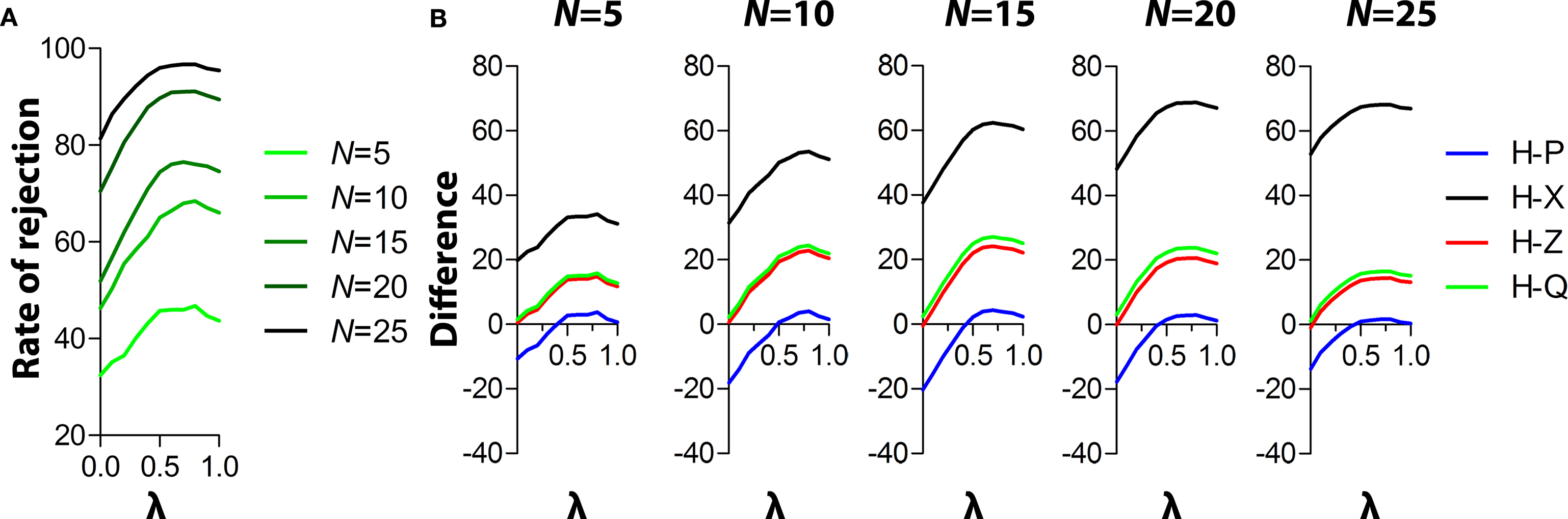
Figure 5. Varying the weighting of Herror and Hpath. (A) Rates of rejection of the null hypothesis are shown for different weights of Herror and Hpath ([λ] and [1 − λ], respectively) for different sample sizes (range 5–25). Hypothesis testing was conducted using the K–S test. Rates of rejection peaked with λ set at 0.8 (for N = 5, 10, 20, 25) and 0.7 (for N = 15), respectively. (B) Relative performance of H vs. other measures at different λ and across N-values ranging from 5 to 25.
Analysis B, Hypothesis Testing for Varying Effect Sizes
The probability of rejecting the null hypothesis (and detecting a difference) depends upon the effect size (i.e., difference between means), as well as the sample size (N) and the variance of the samples. As we sampled from two populations in the above analyses, the effect size was fixed. In order to examine the sensitivity of different measures over a range of effect sizes we compiled three additional databases, each containing 282 probe tests (see also Maei et al., 2009
). These databases were compiled from mice that had all been trained identically (5 days, six trials per day) and then given a series of three probe tests. Performance differed in each of the probe trials (declining from probe 1 → 3). Therefore, comparison of different combinations of probe tests provides an opportunity to evaluate the ability of measures to detect differences over a range of intermediate effect sizes (Figure 6
A). Accordingly, we next performed a series of simulated experiments (as above) and evaluated detection rates for H vs. existing measures using the non-parametric, K–S test (Figure 6
B) (for parallel analyses using the parametric t-test see Figure S4 in Supplementary Material).
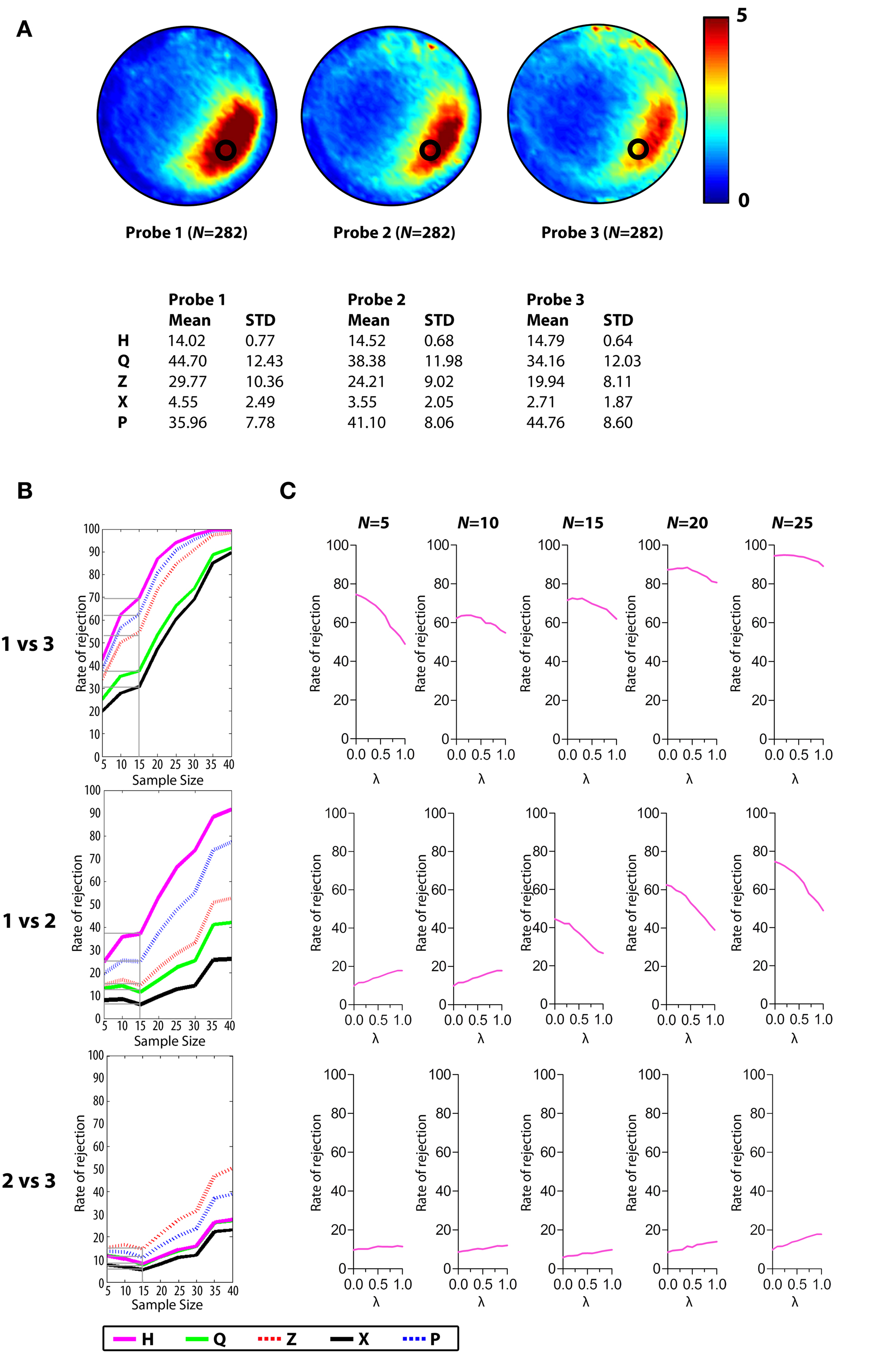
Figure 6. Monte Carlo simulations (Analysis B). Mice were trained in the water maze for 5 days (six trials per day) and then given a series of three probe tests. (A) Density plots for grouped data showing probes 1, 2 and 3. The color scale represents the number of visits per animal per 5 cm × 5 cm area. The table below indicates that performance declined across probe tests, according to all measures. (B) The likelihood of detecting a difference between the probes 1, 2 and 3 datasets is shown for varying sample (N) size, with significance levels α = 0.05, 0.01 and 0.001 using the K–S test. (C) The performance of H at λ varying from 0 to 1.0 in steps of 0.1 with N-values ranging from 5 to 25.
As in our previous analyses, as N increased, detection rates increased for all measures. Importantly, in two of the three comparisons, H outperformed P, Q, Z and X (probe 1 vs. probe 3 and probe 1 vs. probe 2), and its advantage was quite marked. For example, with α set at 0.05 and N = 15, detection rates were highest for H (∼69.8%), compared to P (∼63.4%), Z (∼55.3%), Q (∼36.9%) and X (∼31.5%) for the probe 1 vs. probe 3 comparison. Similarly, detection rates were highest for H (∼37.2%), compared to P (∼25.4%), Z (∼14.2%), Q (∼10.9%) and X (∼6.0%) for the probe 1 vs. probe 2 comparison. For the probe 2 vs. probe 3 comparison, detection rates were close to chance for small-medium sample sizes for all measures [e.g., with α set at 0.05 and N = 15, detection rates ranged from 5.4% (X) to 14.0% (Z)], and H no longer held an advantage over other measures
5
.
Mice in these experiments underwent repeated probe tests, and so the decline in performance from probe 1 to probe 3 likely reflects extinction of a spatial bias (Lattal et al., 2003
; Suzuki et al., 2004
). It is therefore interesting that the advantage of H over existing measures was even more pronounced in the current analysis compared to Analysis A, and this raises the possibility that H may be particularly sensitive to shifts in search strategy that might occur during extinction. In order to explore this issue further, we conducted an additional series of simulations where the relative weighting of Herror and Hpath was varied systematically (Figure 6
C). In contrast to Analysis A, sensitivity generally improved as Hpath weighting increased (for the probe 1 vs. probe 3 and probe 1 vs. probe 2 comparisons), perhaps reflecting the increased incidence of less focused search strategies (e.g., random search, scanning or chaining) (D.P. Wolfer, personal communication; see also Wolfer and Lipp, 2000
; Wolfer et al., 2001
) in the second and third probe tests compared to the first probe test.
Floating Behavior
Mice may occasionally exhibit floating behavior – periods of immobility – during the probe test (for an example see Figure S5 in Supplementary Material). Typically, floating occurs close to the release site and distant from the former platform location. Such behavior would result in high platform error, and, consequently, drive up the composite H score to values comparable to poor (but non-floating) performers.
Experimental Validation of H Index
We next conducted a series of experiments to verify that the H measure can detect spatial learning decrements in mice under a variety of experimental conditions. To do this we used three models of experimentally induced hippocampal dysfunction: (1) complete hippocampal lesions [induced by stereotactic infusion of N-methyl-d-aspartic acid into multiple hippocampal sites (Wang et al., 2009
)], (2) genetic deletion of αCaMKII, a gene implicated in hippocampal behavioral and synaptic plasticity (αCaMKIIΔ mice; Elgersma et al., 2002
) and (3) a mouse model of Alzheimer’s disease [transgenic mice over-expressing two human mutated APP genes associated with early onset of AD; tg-CRND8 mice (Janus et al., 2000
)].
Experiment 1: Extended training protocol (three training trials per day, 11 days)
Mice with complete NMDA-induced hippocampal lesions and sham-operated controls were trained in the water maze with three trials per day over 11 consecutive days. Spatial learning was assessed in probe tests prior to training on days 1, 3, 5, 7, 9 and 11. Histological analyses revealed that neuronal loss was both extensive (>80% of dorsal and ventral hippocampus) and specific (with minimal damage to cortical and thalamic structures adjacent to the hippocampus) (Figure 7
A). As training proceeded, search accuracy in the probe tests improved in control, but not hippocampal-lesioned, mice (Figure 7
B), consistent with previous results (Logue et al., 1997
; Cho et al., 1999
). This transition toward more focal searching in control, but not hippocampal-lesioned, mice was captured by all measures (Figure 7
C). In the probe on day 1, performance in control and hippocampal-lesioned mice was indistinguishable according to all measures. However, as training progressed, eventually all measures began to successfully detect differences in performance between control and hippocampal-lesioned mice. These differences were detected as early as from day 3 by H, Z, X and P and from day 5 by Q.
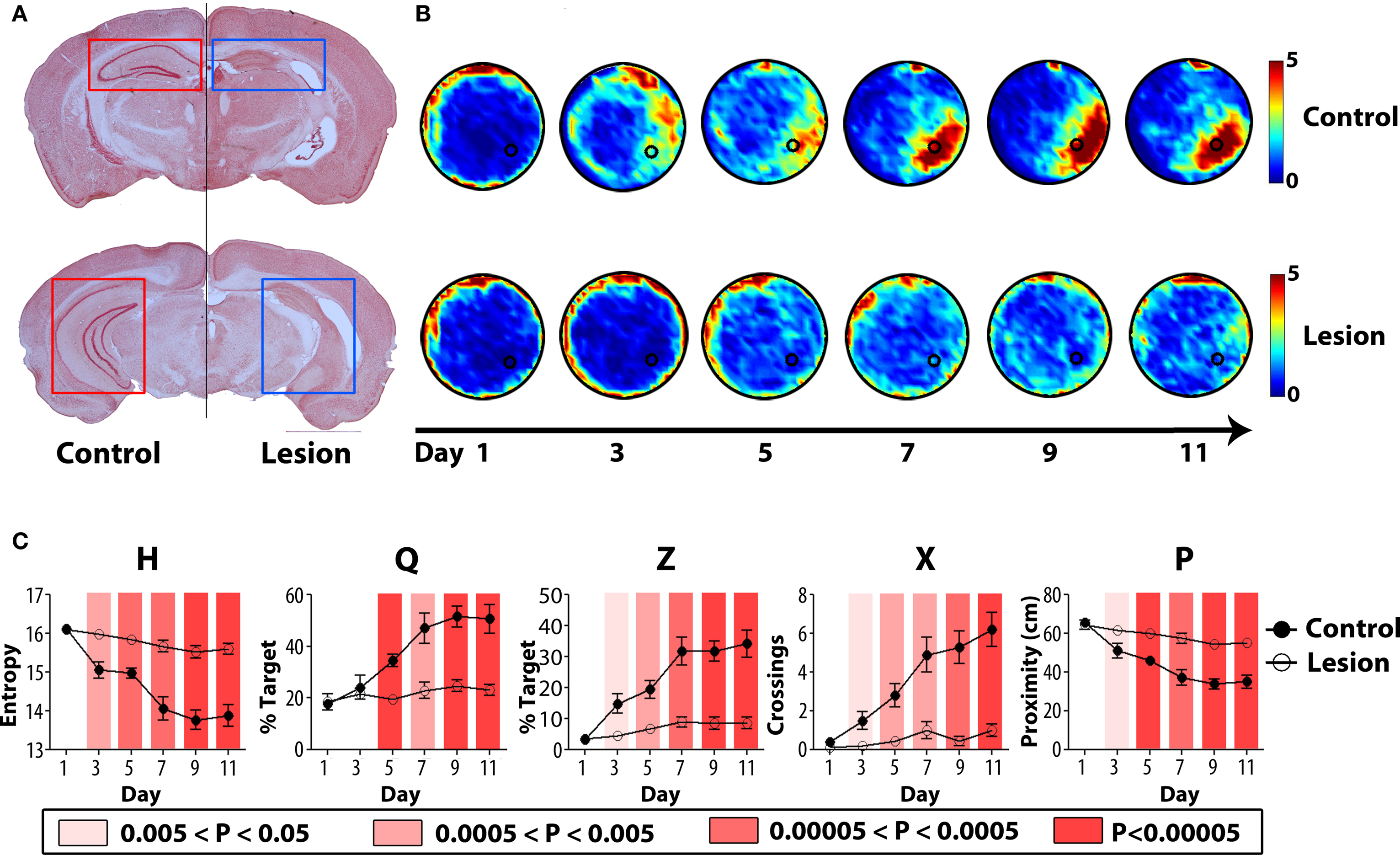
Figure 7. Experimental validation of H (hippocampal lesions). (A) Representative coronal sections of the rostral (top) and caudal (bottom) hippocampus from control (left) and lesioned (right) mice. (B) Mice were trained for 11 days, with probe tests prior to training on days 1, 3, 5, 7, 9, 11. Density plots of probe test performance of control (top) and lesioned (bottom) mice over the course of the 11-day protocol. The color scale represents the number of visits per animal per 5 cm × 5 cm area. (C) Comparison of probe test performance between the two groups computed using H, Q, Z, X, and P using the K–S test. The color-coded bars reflect different P-value ranges.
Experiment 2: Moderate Training Protocol (Six Training Trials Per Day, 3 Days)
In each experiment, mice were trained in the water maze for 3 days (six trials per day) and a probe test was given at the completion of training. Consistent with our results from the extended training protocol, hippocampal-lesioned mice performed significantly worse than control mice in the probe test at the completion of training (Figure 8
A). Similarly, mice with a genetic deletion of αCaMKII (Figure 8
B) or transgenic over-expression of mutated APP genes (Figure 8
C) performed significantly worse than their respective control groups. Most importantly, H was able to detect these spatial learning deficits in each of the three models of experimentally induced hippocampal dysfunction, and together these experiments verify that the H measure can detect spatial learning decrements in mice under a variety of experimental conditions
6
.
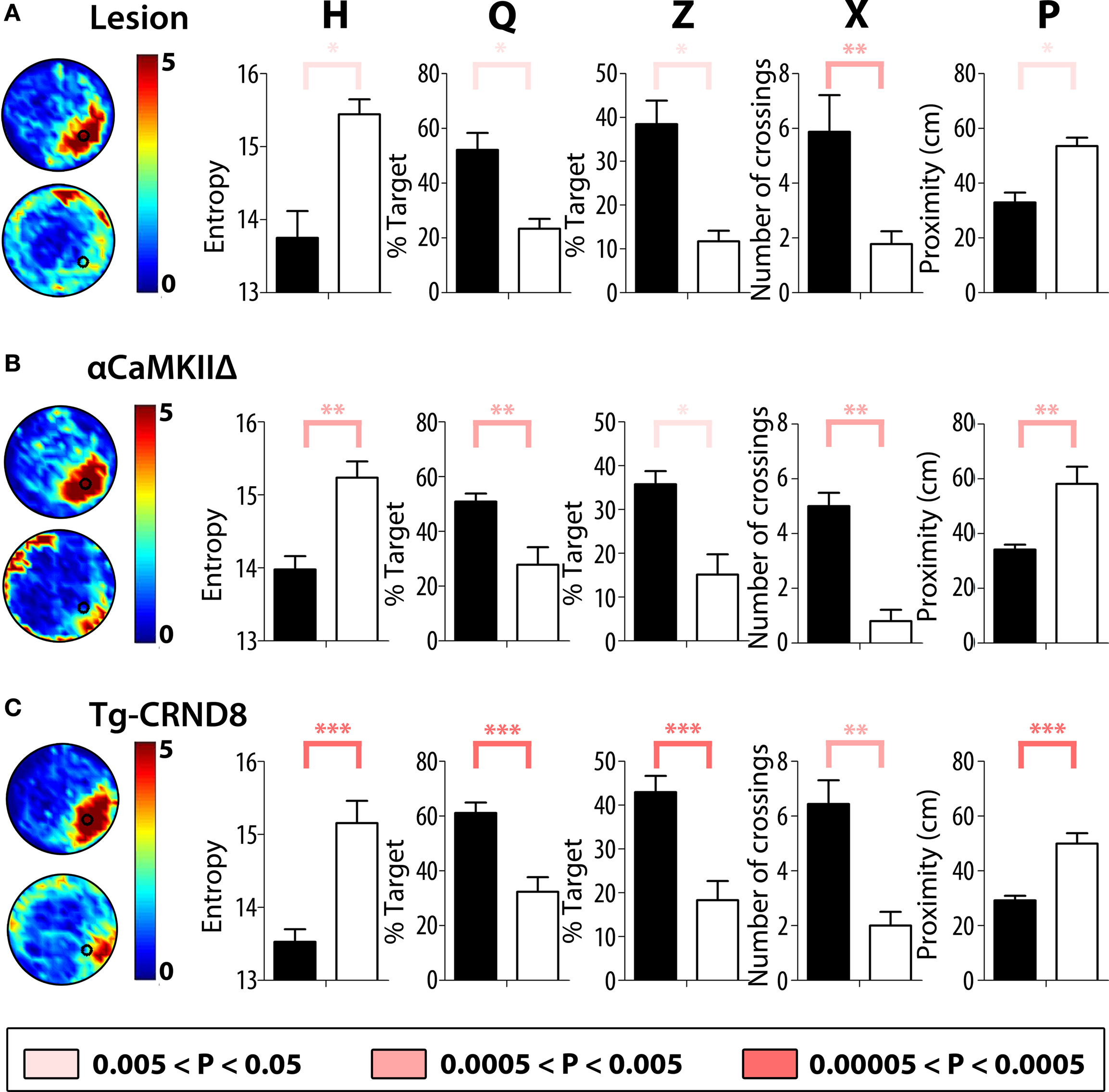
Figure 8. Validation of H with three models of experimentally induced hippocampal dysfunction. In these experiments mice were trained in the water maze for 3 days (six trials per day) and a probe test was given at the completion of training. (A) Left, density plots of probe test performance of control (top) and lesioned (bottom) mice. The color scale represents the number of visits per animal per 5 cm × 5 cm area. Right, comparison of the respective groups using H, Q, Z, X, and P measures. (B) Left, density plots of probe test performance of control WT (top) and αCaMKIIΔ (bottom) mice. Right, comparison of the respective groups using H, Q, Z, X, and P measures. (C) Left, density plots of probe test performance of control WT (top) and tg-CRND8 (bottom) mice. Right, comparison of the respective groups using H, Q, Z, X, and P measures. K–S tests were used for all analyses. * for 0.005 < P < 0.05, ** for 0.0005 < P < 0.005 and *** for 0.00005 < P < 0.0005.
In this paper we developed a new measure to assess water maze probe test performance. Using the concept of entropy, the new H measure considers both the degree to which searching is centered on the former platform location and how focused the search is. We compared the sensitivity of the H measure with four existing measures that are currently used to assess probe test performance. Using this approach, we found that H outperformed existing measures for all sample sizes and most effect sizes, and in many cases by a considerable margin (especially with respect to the most popular of the existing measures, Q). We further validated this new measure using three models of experimentally induced hippocampal dysfunction. Together, these data indicate that H offers greater sensitivity than existing measures, perhaps because it exploits the richness of the precise positional information of the mouse throughout the probe test.
In our analyses we contrasted the H measure with four existing measures that are used in more than 98% of water maze studies (Maei et al., 2009
). Common to all existing measures is that bias for the target location (e.g., south-east) may be contrasted with other equivalent locations in the pool (e.g., north-east, north-west and south-west). Such a within subjects comparison makes it possible to assess whether a particular cohort of mice search selectively (e.g., whether they search more in the south-east quadrant relative to the north-east, north-west and south-west quadrants). However, as control and experimental groups may both search selectively, the more important comparison is whether one group searches more selectively than the other. For this between subjects comparison, relative bias for the target must be contrasted between control and experimental groups, and it is this comparison on which we focused in this study.
Using this approach we found that the new H measure was able to detect group differences with greater sensitivity than existing measures. This was the case under the majority of conditions: Over the full range of sample sizes (i.e., for samples sizes from 5 to 40), and for most effect sizes (the single exception being where both groups are searching poorly). In many instances, the advantage over existing measures was quite striking. For example, for a typical sample size of 15, H held up to a ∼12% point advantage over the next-best performing measure, P, in some scenarios. Compared to the most widely used measure, Q, this advantage was even more marked (up to ∼20–25% points for some scenarios). These analyses, therefore suggest that the implementation of H would significantly improve the efficiency of both low- and high-throughput screening of genetically modified mice. In addition to improved sensitivity, a second attractive feature of the H measure is that it is normally distributed. This is in contrast to the existing measures, which deviate from normality (especially when mice are performing at, or near, floor levels) (Maei et al., 2009
). Because parametric tests (such as the Student’s t-test or analysis of variance) assume that samples are drawn from normally distributed populations, deviations from normality increase the risk of type 1 errors – that is, the likelihood of incorrectly rejecting the null hypothesis may be raised (albeit modestly) when using Q, Z, X or P, but not H.
What might account for the greater sensitivity of the H measure? The superiority of the H measure over existing measures is largely consistent with our hypothesis that measures that more fully exploit the richness of available positional data will be more sensitive. It is noteworthy here that P exhibited the next-best performance across the majority of scenarios, and that both H and P were considerably more sensitive than Q, Z and X. Compared to H and P, these latter measures contain relatively impoverished positional information. Computation of Q and Z, for example, involves a simple determination of whether or not the mouse occupies the region of interest, with all other spatial information discarded. Likewise, for X, the number of times the animal crosses the exact platform location is counted, but all other positional information during the trial is ignored. By contrast, H and P retain more detailed trajectory information. For example, both measures consider deviations of the mouse from the target (i.e., an error signal or d). However, while H uses a measure of dispersion (variance or Herror) as a descriptor of d, P uses a measure of location (i.e., the mean) to describe d. Accordingly, when the relative weighting Herror and Hpath were adjusted so that H was based entirely on Herror, the sensitivity of H and P was quite similar. It is worth noting, however, that H always held a marginal advantage, suggesting that dispersion, rather than location, provides a better descriptor of d
7
.
Where the two measures differ is that H additionally considers variance of the path (or Hpath). The inclusion of this component improved performance considerably, differentiating H from existing measures in a number of different experimental scenarios. Interestingly, the degree to which H outperformed existing measures was sensitive to the relative weighting of Herror and Hpath, and the optimal weighting of these components varied across experimental scenarios. In particular, consideration of Hpath increased sensitivity in Analysis B. As mice in these experiments underwent repeated testing, this suggests that Hpath may be particularly sensitive to changing search strategies that may occur during extinction. However, it is important to note that in our primary analyses we purposefully weighted Herror and Hpath equally. We believe that this offers two advantages. First, it involves fewest assumptions about the relative contributions about these two components to sensitivity (especially since the optimal weighting may vary across experimental settings). Second, it facilitates standardization and comparisons across studies.
The Monte Carlo simulation-based approach that we used to evaluate the sensitivity of the H measure offers three important advantages (see also Maei et al., 2009
). First, large numbers of ‘experiments’ may be simulated, making it possible to compute reliable sensitivity estimates for different measures. In our simulations, sensitivity estimates were based on 10000 ‘experiments’ for each sample size, and with this large number of experiments we were able to detect both subtle and large magnitude differences in sensitivity between measures. Second, the use of relatively large databases (ranging from 282 to 388 probe tests) allowed us to simulate experiments using a wide range of sample sizes (5–40), covering the entire range of sample sizes that would be used in most studies. Third, all probe test data were drawn from experiments that used identical apparatus, training and probe test procedures. Therefore, our simulated experiments closely mimic real experimental situations, as for any given experiment such factors would typically not vary. With respect to this last point, one drawback is also worth noting. The limitation of using identical procedures and apparatus is that it is not certain whether the relative ranking of H, P, Z, Q and X would necessarily hold across a variety of experimental settings. For example, many factors commonly differ across laboratories. These include pool size, size and type of platform, amount of training, external cues, strain and species, and all of which impact performance. While we believe it is reasonable to assume that the ranking of measures would generalize across experimental settings, nonetheless it would be important demonstrate this and, to facilitate this process, we have posted our code
8
(see also Supplemental Material).
In summary, the water maze is one of the most widely used behavioral paradigms for characterization of learning and memory in genetically modified mice. However, since its introduction in the 1980s, surprisingly little attention has been paid to either the optimization of existing measures or the development of new and more sensitive measures. The Q and X measures were introduced in the original water maze studies (Morris, 1981
, 1984
; Morris et al., 1982
) and remain the most popular – being used (either alone or in combination) in roughly 84% of published water maze studies (Maei et al., 2009
). The newer Z and P measures were introduced in the 1990s (Gallagher et al., 1993
; Moser et al., 1993
). However, until recently the relative sensitivity of these measures had not been formally evaluated (Maei et al., 2009
). The goal of the current study was to develop a new measure that would more sensitively evaluate probe test performance and potentially improve the efficiency of behavioral phenotyping. The new measure, based on the concept of entropy, considers both how focused the search is and the degree to which searching is centered on the former platform location. Our series of simulations indicated that H outperformed existing measures over a variety of conditions, and that its advantage was quite marked. More detailed analyses revealed that both the path variance and error variance contributed to the superior sensitivity of H, suggesting that implementation of this measure should lead to more efficient detection of spatial learning phenotypes in genetically engineered mice.
The authors declare that the research was conducted in the absence of any commercial or financial relationships that could be construed as a potential conflict of interest.
This work was supported by grants from the Natural Sciences and Engineering Council Canada to Paul W. Frankland (RGPIN 312434-05) and Sheena A. Josselyn (RGPIN 250250-05). Hamid R. Maei and Afra H. Wang received support from the Research Training Centre at The Hospital for Sick Children. Adelaide P. Yiu received support from Alzheimer’s Society of Canada, and Cátia M. Teixeira received support from the Graduate Program in Areas of Basic and Applied Biology (GABBA) and the Portuguese Foundation for Science and Technology (FCT).
The Supplementary Material for this article can be found online at http://www.frontiersin.org/integrativeneuroscience/paper/10.3389/neuro.07/033.2009/
- ^ All probe tests were screened for general irregularities and probe tests were excluded where (a) there were tracking problems or (b) mice floated.
- ^ Our rationale for combining groups of mice with different experimental manipulations was on the following bases. First, all these experiments used identical procedures and apparatus. Second, each of these manipulations led to profound deficits in performance that were similar in magnitude. However, this represents a practical, rather than perhaps optimal, approach for generating a large dataset for experimentally manipulated mice and we cannot exclude the possibility that there are qualitative differences in the types of disruption produced by each manipulation. That said, while such heterogeneity would make it harder to detect differences between samples drawn from control and experimental datasets, it would not be expected to affect comparisons between measures.
- ^ http://www.mathworks.com/products/matlab/
- ^ We use the F1 generation from a cross between C57B6 and 129svev for two primary reasons: (a) This is the recommended background for transgenic/knockout studies in order to reduce the impact of flanking genes (e.g., Banbury conference on genetic background in mice, 1997 ), and (b) We have found that this particular F1 hybrid (C57B6 × 129svev) is very well suited for water maze studies as they tend to be better learners than the commonly used C57B6 inbred strain (see Logue et al., 1997 ).
- ^ It is likely that under these conditions where both groups are performing poorly path error adds noise to the H measure as increasing the weighting toward platform error improved sensitivity of H significantly (Figure 6 C).
- ^ Of course, differences in spatial performance may not necessarily reflect differences in spatial learning and/or memory. Rather, motor, perceptual, motivational or emotional problems can contribute to impaired performance and so these potential confounds should always be considered when interpreting results from a water maze analysis.
- ^ As for any given trajectory, the distribution of d would be expected to be highly non-Gaussian, the mean likely provides a very poor descriptor of this variable.
- ^ http://individual.utoronto.ca/kpetrov/Matlab-codes.zip
Janus, C., Pearson, J., McLaurin, J., Mathews, P. M., Jiang, Y., Schmidt, S. D., Chishti, M. A., Horne, P., Heslin, D., French, J., Mount, H. T., Nixon, R. A., Mercken, M., Bergeron, C., Fraser, P. E., St George-Hyslop, P., and Westaway, D. (2000). A beta peptide immunization reduces behavioural impairment and plaques in a model of Alzheimer’s disease. Nature 408, 979–982.