Do the Dynamics of Prior Information Depend on Task Context? An Analysis of Optimal Performance and an Empirical Test

In speeded two-choice tasks, optimal performance is prescribed by the drift diffusion model. In this model, prior information or advance knowledge about the correct response can manifest itself as a shift in starting point or as a shift in drift rate criterion. These two mechanisms lead to qualitatively different choice behavior. Analyses of optimal performance (i.e., Bogacz et al., 2006; Hanks et al., 2011) have suggested that bias should manifest itself in starting point when difficulty is fixed over trials, whereas bias should (additionally) manifest itself in drift rate criterion when difficulty is variable over trials. In this article, we challenge the claim that a shift in drift criterion is necessary to perform optimally in a biased decision environment with variable stimulus difficulty. This paper consists of two parts. Firstly, we demonstrate that optimal behavior for biased decision problems is prescribed by a shift in starting point, irrespective of variability in stimulus difficulty. Secondly, we present empirical data which show that decision makers do not adopt different strategies when dealing with bias in conditions of fixed or variable across-trial stimulus difficulty. We also perform a test of specific influence for drift rate variability.

Introduction

In real-life decision making, people often have a priori preferences for and against certain choice alternatives. For instance, some people may prefer Audi to Mercedes, Mac to PC, or Gillette to Wilkinson, even before seeing the product specification. For product preferences, people are influenced by prior experiences and advertising. Here we study the effects of prior information in the context of perceptual decision making, where participants have to decide quickly whether a cloud of dots is moving to the left or to the right. Crucially, participants are given advance information about the likely direction of the dots. In the experiment reported below, for instance, participants were sometimes told that 80% of the stimuli will be moving to the right. How does this advance information influence decision making?

In general, advance information that favors one choice alternative over the other biases the decision process: people will prefer the choice alternative that has a higher prior probability of being correct. This bias usually manifests itself as a shorter response time (RT) and a higher proportion correct when compared to a decision process with equal prior probabilities. Because bias expresses itself in two dependent variables simultaneously (i.e., RT and proportion correct), and because people only have control over a specific subset of the decision environment (e.g., the participant cannot control task difficulty) an analysis of optimal adjustments is traditionally carried out in the context of a sequential sampling model. Prototypical sequential sampling models such as the Sequential Probability Ratio Test (SPRT; e.g., Wald and Wolfowitz, 1948; Laming, 1968) or the drift diffusion model (DDM; Ratcliff, 1978) are based on the assumption that the decision maker gradually accumulates noisy information until an evidence threshold is reached.

In such sequential sampling models, the biasing influence of prior knowledge can manifest itself in two ways (e.g., Diederich and Busemeyer, 2006; Ratcliff and McKoon, 2008; Mulder et al., 2012). The first manifestation, which we call prior bias, is that a decision maker decides in advance of the information accumulation process to lower the evidence threshold for the biased alternative. The second manifestation, which we call dynamic bias (cf. Hanks et al., 2011), is that a decision maker weighs more heavily the evidence accumulated in favor of the biased alternative. There is both theoretical and empirical evidence that shows that both types of bias manifest itself in different situations.

The situation that has been studied most often is one in which task difficulty is fixed across trials. For this case, Edwards (1965) has shown that optimal performance can be achieved by prior bias alone. In empirical support for this theoretical analysis, Bogacz et al. (2006) demonstrated that in three experiments the performance of participants approximated the optimality criterion from Edwards (1965). In a recent paper by Gao et al. (2011), it was demonstrated that for fixed stimulus difficulty, but varied response deadlines over trials, behavioral data was best described by the implementation of prior bias.

Another situation is one in which task difficulty varies across trials. For this case, Hanks et al. (2011) reasoned that people should tend ever more strongly toward the biased response option as the information accumulation process continues (see also Yang et al., 2005; Bogacz et al., 2006, p. 730). The intuitive argument is that a lengthy decision process indicates that the decision is difficult (i.e., the stimulus does not possess much diagnostic information), and this makes it adaptive to attach more importance to the advance information. In the extreme case, a particular stimulus can be so difficult that it is better to simply go with the advance information and guess that the biased response option is the correct answer.

Thus, in an environment of constant difficulty an optimal decision maker accommodates advance information by prior bias alone, such that a choice for the likely choice alternative requires less evidence than that for the unlikely choice alternative. The conjecture of Hanks et al. (2011) is that, in an environment of variable difficulty, an optimal decision maker accommodates advance information not just by prior bias, but also by dynamic bias.

This paper has two main goals. The first goal is to extend the analytical work of Edwards (1965) and show that prior bias accounts for optimal performance regardless of whether stimulus difficulty is fixed or variable across trials. The second goal is to examine empirically which kind of bias decision makers implement when stimulus difficulty is fixed or variable.

The organization of the paper is as follows. In the first section we briefly introduce the drift diffusion model (DDM), the prototypical sequential sampling model that can be used to model both prior bias and dynamic bias (Bogacz et al., 2006; van Ravenzwaaij et al., 2012). Next we present analytical work that shows how optimal performance in biased decision environments may be achieved with prior bias alone, regardless of whether stimulus difficulty is fixed or variable. We then present an empirical study showing how people accommodate bias for fixed and variable stimulus difficulty in similar fashion.

The Drift Diffusion Model (DDM)

In the DDM (Ratcliff, 1978; Ratcliff and Rouder, 2000; Wagenmakers, 2009; van Ravenzwaaij et al., 2012), a decision process with two response alternatives is conceptualized as the accumulation of noisy evidence over time. Evidence is represented by a single accumulator, so that evidence in favor of one alternative is evidence against the other alternative. A response is initiated when the accumulated evidence reaches one of two predefined thresholds. For instance, in a lexical decision task, participants have to decide whether a letter string is an English word, such as TANGO, or a non-word, such as TANAG (Figure 1).

FIGURE 1

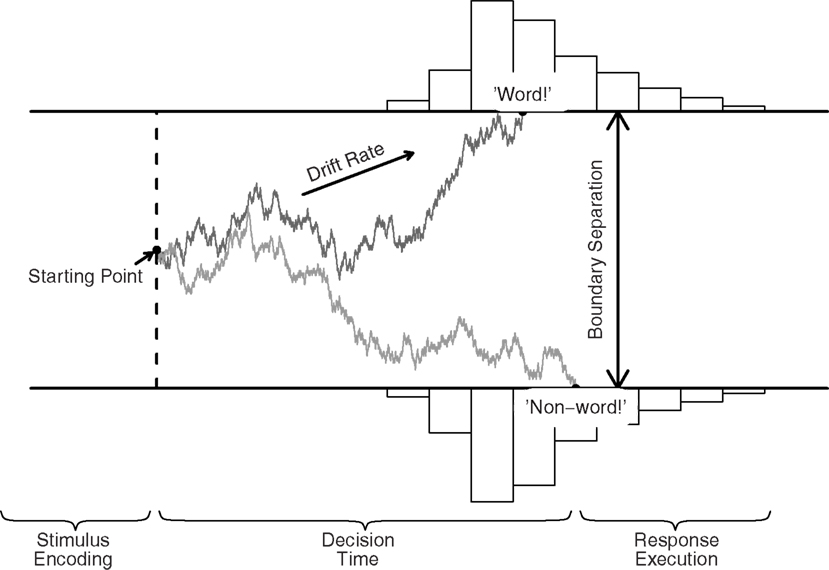
Figure 1. The DDM and its key parameters, illustrated for a lexical decision task. Evidence accumulation begins at starting point z, proceeds over time guided by mean drift rate v, but subject to random noise, and stops when either the upper or the lower boundary is reached. Boundary separation a quantifies response caution. The predicted RT equals the accumulation time plus the time required for non-decision processes T_er (i.e., stimulus encoding and response execution).

The model assumes that the decision process commences at the starting point z, from which point evidence is accumulated with a signal-to-noise ratio that is governed by mean drift rate v and Wiener noise. Without trial-to-trial variability in drift rate, the change in evidence x is described by the following stochastic differential equation

$dx\left(t\right)=v\cdot dt+s\cdot dW\left(t\right),$(1)

where W represents the Wiener noise process (i.e., idealized Brownian motion). Parameter s represents the standard deviation of dW(t)¹. Values of v near zero produce long RTs and high error rates. Trial-to-trial variability in drift rate is quantified by η.

Evidence accumulation stops and a decision is initiated once the evidence accumulator hits one of two response boundaries. The difference between these boundaries, boundary separation a, determines the speed–accuracy trade-off; lowering a leads to faster RTs at the cost of a higher error rate. When the starting point, z, is set at a/2, bias in the decision process is not manifested in the starting point. Together, these parameters generate a distribution of decision times (DTs). The observed RT, however, also consists of stimulus-non-specific components such as response preparation and motor execution, which together make up non-decision time T_er. The model assumes that T_er simply shifts the distribution of DT, such that RT = DT + T_er (Luce, 1986).

Thus, the five key parameters of the DDM are (1 and 2) speed of information processing, quantified by mean drift rate v and standard deviation of drift rate η; (3) response caution, quantified by boundary separation a; (4) evidence criterion, quantified by starting point z; and (5) non-decision time, quantified by T_er. In addition to these five parameters, the full DDM also includes parameters that specify across-trial variability in starting point, and non-decision time (Ratcliff and Tuerlinckx, 2002).

Bias in the DDM

Recall from the introduction that decision makers may implement bias in two ways. A decision maker may decide prior to the start of the decision process that less evidence is required for a response in favor of the biased alternative than for the non-biased alternative. This type of bias, which we call prior bias, is manifested in the DDM as a shift in starting point (see the top panel of Figure 2, see also Ratcliff, 1985; Ratcliff and McKoon, 2008; Mulder et al., 2012). Prior bias is most pronounced at the onset of the decision process, but dissipates over time due to the effects of the diffusion noise s. Edwards (1965) showed that when across-trial stimulus difficulty is fixed, it is optimal to shift the starting point an amount proportional to the odds of the prior probabilities of each response alternative.

FIGURE 2

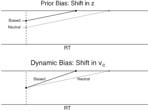
Figure 2. Schematic representation of bias due to a shift in starting point z (top panel) or a shift in drift rate criterion v_c (bottom panel). The gray lines represent neutral stimuli for comparison.

Alternatively, a decision maker may weigh evidence in favor of the biased response alternative more heavily than evidence in favor of the non-biased response alternative. This type of bias, which we call dynamic bias, is manifested in the DDM as a shift in drift rate criterion (see the bottom panel of Figure 2, see also Ratcliff, 1985; Ratcliff and McKoon, 2008; Mulder et al., 2012). With a shift in the drift rate criterion, drift rate for the likely choice alternative is enhanced by a bias component, such that the cumulative effect of dynamic bias grows stronger over time (compare the difference between the biased and neutral lines for shift in z and shift in v_c).

Bias in Theory

Below, we examine analytically which DDM parameter shifts in starting point and drift rate criterion produce optimal performance. We differentiate between fixed and variable difficulty. Two criteria of optimality are discussed: highest mean proportion correct when there is a fixed response deadline (i.e., the interrogation paradigm) and lowest mean RT (MRT) for a fixed mean proportion correct (see also Bogacz et al., 2006). In the next section, we discuss highest mean proportion correct for the interrogation paradigm.

Optimality Analysis I: The Interrogation Paradigm

In the interrogation paradigm, participants are presented with a stimulus for a fixed period of time. Once the response deadline T is reached, participants are required to immediately make a response (see Figure 3). Thus, for the interrogation paradigm, there are no response boundaries. As such, the unbiased starting point z is 0. In this section, we will look at optimal DDM parameter settings for a biased decision in the interrogation paradigm. The performance criterion is the mean proportion correct. First, we discuss fixed stimulus difficulty across trials, or η = 0. Second, we discuss variable stimulus difficulty across trials, or η > 0.

FIGURE 3

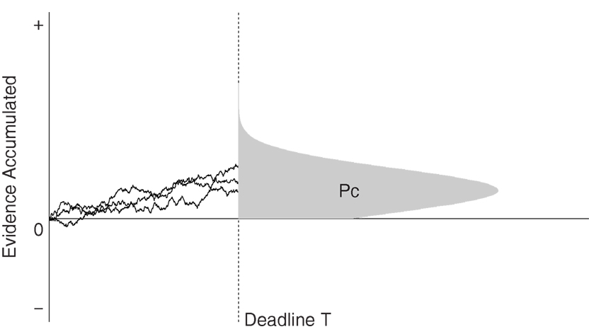
Figure 3. The interrogation paradigm. At deadline T, decision makers choose a response alternative depending on the sign of the evidence accumulator. The shaded area under the distribution represents the proportion of correct answers.

Fixed difficulty

In order to find the maximum mean proportion correct for the interrogation paradigm, we assume that participants base their response depending on whether the evidence accumulator is above or below zero when the accumulation process is interrupted (see, e.g., van Ravenzwaaij et al., 2011; Figure 9). We choose parameter settings such that if the accumulator is above zero at time T, the biased response is given, whereas if the accumulator is below zero at time T, the non-biased response is given.

Across trials, the final point of the evidence accumulator will be normally distributed with mean vT + z and standard deviation $s\sqrt{T}$ (e.g., Bogacz et al., 2006; van Ravenzwaaij et al., 2011). In what follows, we assume that stimuli corresponding to either of the two response alternatives are equally difficult². For fixed difficulty, the analytical expression for mean proportion correct for an unbiased decision in the interrogation paradigm, denoted by PcI_F,U, is given by

$Pc{I}_{F,U}=\Phi \left[\frac{vT+z}{s\sqrt{T}}\right],$(2)

where Φ denotes the standard normal cumulative distribution³. In PcI_F,U, the I denotes “Interrogation,” the F denotes “Fixed Difficulty,” and the U denotes “Unbiased.” For a biased decision, this expression becomes:

$Pc{I}_{F,B}=\beta \Phi \left[\frac{\left(v+v_c\right)T+z}{s\sqrt{T}}\right]+\left(1-\beta \right)\Phi \left[\frac{\left(v-v_c\right)T-z}{s\sqrt{T}}\right].$(3)

where β denotes the proportion of stimuli that are consistent with the prior information (i.e., in the experiment below, β = 0.80) and v_c denotes the shift in drift rate criterion. In PcI_F,B, the I denotes “Interrogation,” the F denotes “Fixed Difficulty,” and the B denotes “Biased.” Equation (3) is derived from equation (2) as follows. To incorporate a shift in starting point z toward the biased alternative, the left-hand side of equation (3) contains z (cf. equation (2)). In the right-hand side, z is replaced by −z to account for the fact that the correct answer lies at the non-biased threshold. To incorporate a shift in drift rate criterion, the left-hand side of equation (3) adds a shift v_c to mean drift rate v. In the right-hand side, the shift v_c is subtracted from mean drift rate v.

Maxima for PcI_F,B occur for:

$z_{max}+v_c\cdot T=\frac{s^{2}log\left(\frac{\beta }{1-\beta }\right)}{2v},$(4)

where z_max denotes the value of the starting point that leads to the highest PcI_F,B (e.g., Edwards, 1965; Bogacz et al., 2006, for expressions without v_c·T).

The addition of v_c·T to the left-hand side of equation (4) follows from inspection of both numerators in equation (3): it shows a trade-off between the starting point z and the shift in drift rate criterion v_c, such that Δz = Δv_c·T, where Δ denotes a parameter shift. Therefore, the maximum value of PcI_F,B does not belong to a unique set of parameters, but exists along an infinite combination of values for z and v_c. This trade-off is graphically displayed for different sets of parameter values in Figure 4.

FIGURE 4

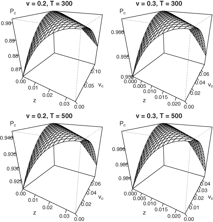
Figure 4. Mean percentage correct for fixed difficulty (η = 0) in the interrogation paradigm for different combinations of starting point z and shift in mean drift rate v_c. Due to the trade-off Δz = Δv_c·T, no unique maximum exists.

Figure 4 shows that for a drift rate v of 0.2 or 0.3, combined with a deadline T of 300 or 500 ms, every maximum that occurs for a particular value of z with v_c = 0 may also be reached for different combinations of z and v_c (bias β is set to 0.8). Results for different sets of parameters look qualitatively similar.

Taken at face value, this result challenges the claim that optimal behavior in biased decision problems is exclusively accomplished by a shift in starting point z: the same level of accuracy may be accomplished by, for instance, setting z = 0 and v_c = z_max/T or any other combination of values that is consistent with the parameter trade-off Δz = Δv_c·T. Importantly, however, participants have to be aware of the exact moment of the deadline T to be able to utilize the trade-off between starting point and drift rate criterion. Recent work by Gao et al. (2011) examined the type of bias people implement when the deadline T is varied across blocks of trials, so that exact knowledge of the deadline is absent. The authors used the leaky competing accumulator model (LCA), a model akin to the DDM with separate accumulators for each response alternative. Using the LCA, the authors were able to differentiate between dynamic bias (shift in the input of the biased accumulator), and two accounts of prior bias (shift in starting point of the biased accumulator and shift in response threshold of the biased accumulator). The results showed that for varying deadline T, people implement a shift in starting point for the biased accumulator. This is indicative of prior bias.

Next, we examine optimal decision making in the interrogation paradigm when participants have no a priori knowledge of the difficulty of the decision problem. In other words, stimulus difficulty varies across trials.

Variable difficulty

To obtain an expression for the mean proportion correct in the interrogation paradigm when there is across-trial variability in stimulus difficulty, it is necessary to include across-trial variability in drift rate, or η. The mean proportion correct for this situation, or PcI_V,B, is derived by multiplying equation (3) by a Gaussian distribution of drift rates with mean v and standard deviation η. The resulting expression needs to be integrated over the interval (−∞, ∞) with respect to drift rate ξ:

$Pc{I}_{V,B}={\int }_{-\infty }^{\infty }\left(\beta \Phi \left[\frac{\left(\xi +v_c\right)T+z}{s\sqrt{T}}\right]+\left(1-\beta \right)\Phi \right.\left.\times \left[\frac{\left(\xi -v_c\right)T-z}{s\sqrt{T}}\right]\right)\frac{1}{\sqrt{2\pi {\eta }^2}}exp\left(-\frac{{\left(\xi -v\right)}^2}{2{\eta }^2}\right)d\xi ,$(5)

which simplifies to

$\begin{array}{l}Pc{I}_{V,B}=\beta \Phi \left[\frac{\left(v+v_c\right)T+z}{\sqrt[s]{T+T^2{\eta }^2/s^2}}\right]\\ +\left(1-\beta \right)\Phi \left[\frac{\left(v-v_c\right)T-z}{\sqrt[s]{T+T^2{\eta }^2/s^2}}\right].\end{array}$(6)

In PcI_V,B, the I denotes “Interrogation,” the V denotes “Variable Difficulty,” and the B denotes “Biased.” The derivation can be found in the appendix.

By differentiating with respect to z in a way analogous to the derivation of equation (4) from equation (3), maxima for PcI_V,B occur for:

$z_{max}+v_c\cdot T=\frac{\left(s^2+{\eta }^{2}T\right)log\left(\frac{\beta }{1-\beta }\right)}{2v},$(7)

where z_max denotes the value of the starting point that leads to the highest PcI_V,B.

Once again, the addition of v_c·T to the left-hand side of equation (7) follows from inspection of both numerators in equation (6): it shows a trade-off between the starting point z and the shift in drift rate criterion v_c, such that Δz = Δv_c·T, where Δ denotes a parameter shift. Figure 5 graphically displays the parameter trade-off for the same sets of parameter values that were used in Figure 4 (η is set to 0.1). Results for different sets of parameters look qualitatively similar.

FIGURE 5

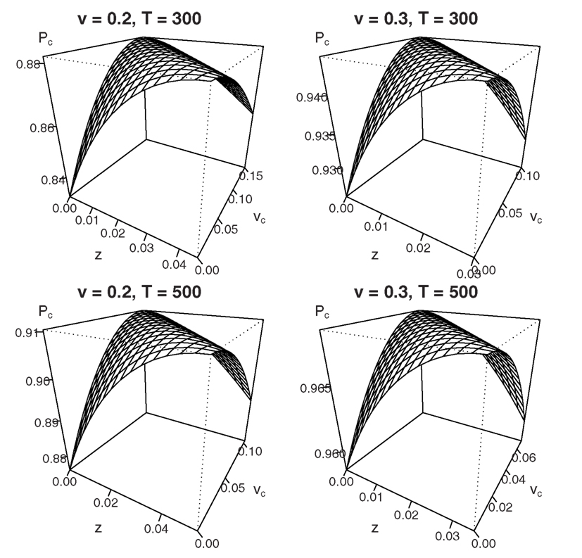
Figure 5. Mean percentage correct for variable difficulty (η = 0.1) in the interrogation paradigm for different combinations of starting point z and shift in mean drift rate v_c. Due to the trade-off Δz = Δv_c·T, no unique maximum exists.

In sum, our derivations and figures show that in the interrogation paradigm with variable across-trial stimulus difficulty, optimal decisions may again be reached by shifting either starting point z, drift rate criterion v_c, or a combination of the two. For an Ornstein–Uhlenbeck process, the fact that both types of bias cannot be distinguished in the interrogation paradigm for both fixed and variable stimulus difficulty had already been demonstrated (Feng et al., 2009, see also Rorie et al., 2010). Contrary to the fixed difficulty situation, however, participants need to know the value of deadline T to optimize performance even when just shifting starting point.

As noted in the introduction, Hanks et al. (2011) suggested that bias should manifest itself as shifts in both starting point and the drift rate criterion when stimulus difficulty varies over trials. The authors reasoned that decision makers should decide in favor of the biased alternative when the decision process is lengthy, because slow decisions are likely to be difficult decisions. However, in the interrogation paradigm, all decisions take equally long. In order to more thoroughly investigate the claim of Hanks et al. (2011), it is necessary to eliminate the deadline T and examine a different criterion of optimality: minimum MRT for a fixed percentage correct.

Optimality Analysis II: Minimum MRT for Fixed Accuracy

In this section we consider the minimum mean RT for fixed accuracy in a free response paradigm. In the free response paradigm, a response is made once the evidence accumulator hits an upper boundary a or a lower boundary 0; the unbiased starting point z is a/2. First, we discuss the situation in which across-trial stimulus difficulty is fixed.

Fixed difficulty

In order to find the minimum MRT for a given level of accuracy, we need expressions for both MRT and accuracy in the DDM for a biased decision. We can then calculate combinations of starting point z and drift criterion shift v_c that yield a given level of accuracy for a given set of parameter values for drift rate v, boundary separation a, and diffusion noise s. The last step is to calculate the MRT for each combination of starting point z and drift criterion shift v_c.

For fixed difficulty, the analytical expression for mean proportion correct for an unbiased decision without a deadline, denoted by Pc_F,U, is given by

$P{c}_{F,U}=\frac{\exp \left(\frac{2av}{s^2}\right)-\exp \left(\frac{2\left(a-z\right)v}{s^2}\right)}{\exp \left(\frac{2av}{s^2}\right)-1},$(8)

(see, e.g., Wagenmakers et al., 2007, equation (2))⁴. In Pc_F,U, the F denotes “Fixed Difficulty,” and the U denotes “Unbiased.” Transforming equation (8) to an expression for a biased decision occurs in a similar fashion as the derivation of equation (3) from equation (2):

$P{c}_{F,B}=\beta Pc{+}_{F,B}+\left(1-\beta \right)Pc{-}_{F,B},$(9)

where

$\begin{array}{l}Pc{+}_{F,B}=\left[\frac{\exp \left(\frac{2a\left(v+v_c\right)}{s^2}\right)-\exp \left(\frac{2\left(a-z\right)\left(v+v_c\right)}{s^2}\right)}{\exp \left(\frac{2a\left(v+v_c\right)}{s^2}\right)-1}\right]\\ Pc{-}_{F,B}=\left[\frac{\exp \left(\frac{2a\left(v-v_c\right)}{s^2}\right)-\exp \left(\frac{2z\left(v-v_c\right)}{s^2}\right)}{\exp \left(\frac{2a\left(v-v_c\right)}{s^2}\right)-1}\right].\end{array}$(10)

In Pc_F,B, the B denotes “Biased.”

To incorporate a shift in starting point z toward the biased alternative, Pc + _F,B contains z as in equation (8). For Pc − _F,B, z is replaced by a − z to account for the fact that the correct answer lies at the non-biased threshold. To incorporate a shift in drift rate criterion, Pc + _F,B adds a shift v_c to mean drift rate v. For Pc − _F,B, the shift v_c is subtracted from mean drift rate v.

Now that we have an expression for mean proportion correct for a biased decision without a response deadline, we need an expression for MRT. For an unbiased decision without deadline, MRT is given by

$MR{T}_U=-\frac{z}{v}+\frac{a\left[exp\left(-2vz∕s^2\right)-1\right]}{v\left[exp\left(-2va∕s^2\right)-1\right]},$(11)

(e.g., Grasman et al., 2009, equation (5)). For a biased decision, this expression becomes

$\begin{array}{c}MR{T}_B=\beta \left(-\frac{z}{v+vc}+\frac{a\left[exp\left(-2\left(v+vc\right)z∕s^2\right)-1\right]}{\left(v+vc\right)\left[exp\left(-2\left(v+vc\right)a∕s^2\right)-1\right]}\right)\\ +\left(1-\beta \right)\left(-\frac{a-z}{v-vc}+\frac{a\left[exp\left(-2\left(v-vc\right)\left(a-z\right)∕s^2\right)-1\right]}{\left(v-vc\right)\left[exp\left(-2\left(v-vc\right)a∕s^2\right)-1\right]}\right).\end{array}$(12)

In what follows, we will fix Pc_F,B to two percentages (i.e., 90 and 95%). Then, we calculate MRT_B for each combination of starting point z and drift rate criterion v_c that yields the predetermined value of Pc_F,B and determine which combination is optimal in the sense that it results in the lowest MRT_B.

Firstly we considered the following set of parameters: mean drift rate v = 0.2, boundary separation a = 0.12, and bias β = 0.8⁵. The top-left panel of Figure 6 shows that an accuracy level of 90% may be achieved by a combination of shifts for starting point z and shifts of drift rate criterion v_c. Again, both parameters exist in a trade-off relationship, such that higher values of z combined with lower values of v_c produce the same mean proportion correct.

FIGURE 6

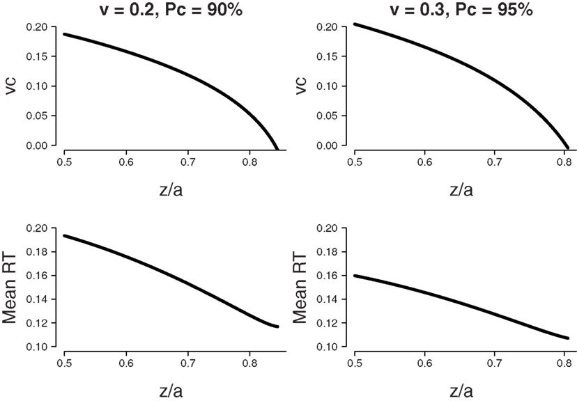
Figure 6. Fixed difficulty (η = 0) in the free response paradigm. Minimum MRT is achieved when all bias is accounted for by a shift in starting point z. Bias β = 0.8, boundary separation a = 0.12. Top panel: Parameter combinations of starting point as a ratio of boundary separation z/a and shift in drift rate criterion v_c that lead to the same fixed level of accuracy (90% for v = 0.2, 95% for v = 0.3). Bottom panel: Mean RT that corresponds to the parameter combinations of the top panel.

The bottom-left panel of Figure 6 shows MRT for each calculated combination of starting point z and drift rate criterion v_c. The x-axis shows the value for starting point z (as a proportion of boundary separation a), the associated value for drift rate criterion v_c can be found in the top-left panel. The MRT results show that the lowest value for MRT is reached when all bias is accounted for by a shift in starting point z.

Secondly we considered a mean drift rate v = 0.3 and an accuracy level of 95%. The results, shown in the right two panels of Figure 6, are qualitatively similar⁶.

In sum, when there is no response deadline and across-trial difficulty is fixed, the optimal way to deal with bias is by shifting the starting point toward the biased response alternative, without shifting the drift rate criterion. In an empirical paper by Simen et al. (2009), it was demonstrated that human participants do indeed shift starting point toward the biased response alternative. No explicit mention of shifts in drift rate criterion are made. In the next subsection, we examine optimal performance for variable stimulus difficulty across trials.

Variable difficulty

Unfortunately, for variable difficulty there are no expressions for mean percentage correct and MRT. As such, we approximate the results for fixed difficulty by numerically obtaining combinations of starting point z and drift rate criterion v_c that yield two percentages correct (i.e., 90 and 95%). Then, we determine which combination is optimal in the sense that it results in the lowest MRT.

The top-left panel of Figure 7 shows the set of parameter values of starting point z and drift rate shift v_c that lead to a percentage correct of 90% with a mean drift rate v = 0.2. The top-right panel shows the set of parameter values of starting point z and drift rate shift v_c that lead to a percentage correct of 95% with a mean drift rate v = 0.3. For both panels, boundary separation a = 0.12, bias β = 0.8, and standard deviation of drift rate η = 0.1. The bottom panels of Figure 7 show corresponding values of MRT. The MRT results show that as for fixed difficulty, the lowest value for MRT is reached when all bias is accounted for by a shift in starting point z.

FIGURE 7

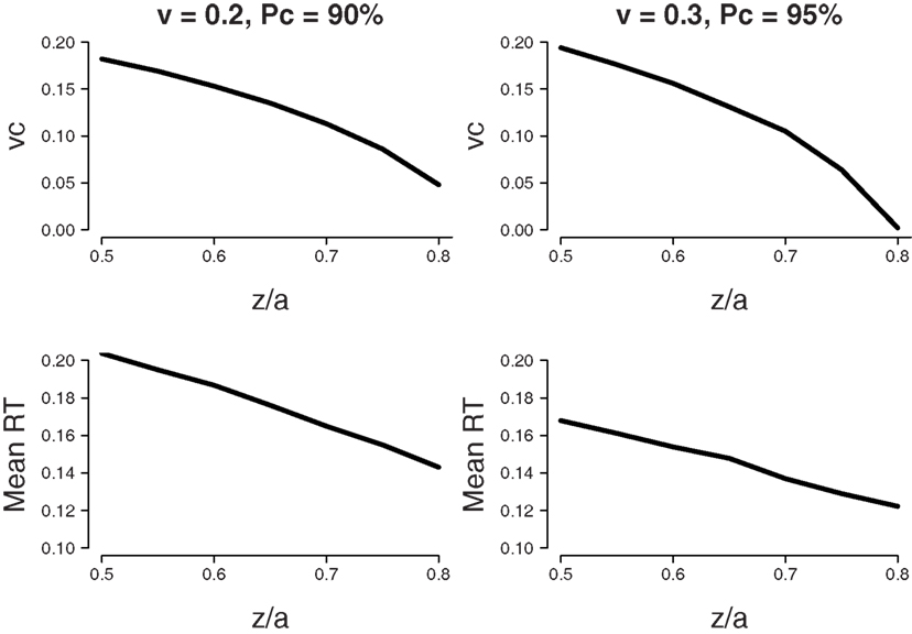
Figure 7. Variable difficulty (η = 0.1) in the free response paradigm. Minimum MRT is achieved when all bias is accounted for by a shift in starting point z. Bias β = 0.8, boundary separation a = 0.12. Top panel: Parameter combinations of starting point as a ratio of boundary separation z/a and shift in drift rate criterion v_c that lead to the same fixed level of accuracy (90% for v = 0.2, 95% for v = 0.3). Bottom panel: Mean RT that corresponds to the parameter combinations of the top panel.

In sum, in paradigms with variable across-trial difficulty, but no response deadline, the optimal way to deal with bias is by shifting the starting point toward the biased response alternative, without shifting the drift rate criterion. This result mirrors the result for fixed difficulty.

Interim conclusion

Hanks et al. (2011) claimed that for biased decisions with variable across-trial stimulus difficulty, optimal performance requires not just a shift in starting point but also a shift in drift rate criterion (i.e., dynamic bias). Our results challenge this claim: regardless of whether stimulus difficulty is fixed or variable, optimal performance can be obtained by having bias only shift the starting point, and not the drift rate criterion. In the next section, we will investigate how people perform in practice.

Bias in Practice

We have demonstrated that optimal performance in decision conditions with a biased response alternative can be achieved by shifting only the starting point criterion. However, people may not accommodate bias in an optimal manner. For instance, Hanks et al. (2011) demonstrated that in a decision environment with variable across-trial stimulus difficulty, participants accommodate advance information by dynamic bias. The authors did not, however, directly compare the performance of participants in conditions with fixed and variable across-trial stimulus difficulty. In this section, we perform such a comparison and address the question whether the inclusion of variability in stimulus difficulty alters the way in which people accommodate advance information. We also examine if the performance of people in practice corresponds to the theoretical optimality indicated in the previous sections.

Our experiment also allows us to test a prediction from the DDM, namely that increasing the variability in across-trial stimulus difficulty results in a higher estimate of across-trial drift rate variability η. The experiment used a random dot motion task (Newsome et al., 1989) with advance information about the upcoming direction of movement. In a within-subjects design, each participant was administered a condition with fixed stimulus difficulty (i.e., identical coherence of movement from trial-to-trial) and a condition with variable stimulus difficulty (i.e., variable coherence).

Participants

Eleven healthy participants (8 female), aged 19–40 years (mean 24.6) performed a random-dots motion (RDM) paradigm in exchange for course credit or a monetary reward of 28 euros. Participants were recruited through the University of Amsterdam and had normal or corrected-to-normal vision. The procedure was approved by the ethical review board at the University of Amsterdam and informed consent was obtained from each participant. According to self-report, no participant had a history of neurological, major medical, or psychiatric disorder.

Materials

Participants performed an RT version of an RDM task. Participants were instructed to maintain fixation on a cross at the middle of the screen and decide the direction of motion of a cloud of partially randomly moving white dots on a black background. The decision was made at any time during motion viewing with a left or right button press. The stimulus remained on screen until a choice was made. The motion stimuli were similar to those used elsewhere (e.g., Newsome and Paré, 1988; Britten et al., 1992; Gold and Shadlen, 2003; Palmer et al., 2005; Ratcliff and McKoon, 2008; Mulder et al., 2010): white dots, with a size of 3 × 3 pixels, moved within a circle with diameter of 5° with a speed of 5°/s and a density of 16.7 dots/degree²/s on a black background. On the first three frames of the motion stimulus, the dots were located in random positions. For each of these frames the dots were repositioned after two subsequent frames (the dots in frame one were repositioned in frame four, the dots in frame two were repositioned in frame five, etc.). For each dot, the new location was either random or in line with the motion direction. The probability that a dot moved coherent with the motion direction is defined as coherence. For example, at a coherence of 50%, each dot had a probability of 50% to participate in the motion–stimulus, every third frame (see also Britten et al., 1992; Gold and Shadlen, 2003; Palmer et al., 2005).

Visual stimuli were generated on a personal computer (Intel Core2 Quad 2.66 GHz processor, 3 GB RAM, two graphical cards: nvidia GeForce 8400 GS and a nvidia GeForce 9500 GT, running MS Windows XP SP3) using custom software and the Psychophysics Toolbox Version 3.0.8 (Brainard, 1997) for Matlab (version 2007b, Mathworks, 1984).

Difficulty

To get acquainted with the task, each participant performed a practice block of 40 easy trials (60% coherence). To match the difficulty level of the motion stimuli across participants, each participant performed an additional block of 400 trials of randomly interleaved stimuli with different motion strengths (resp. 0, 10, 20, 40, and 80% coherence, 80 trials each). We fitted the DDM to the mean response times and accuracy data of this block using a maximum likelihood procedure, constraining the drift rates to be proportional to the coherence settings (Palmer et al., 2005). For each participant, the motion strength at 75% accuracy was then interpolated from the psychometric curve (predicted by the proportional-rate diffusion model) and used in the experimental blocks with fixed coherence across trials. For blocks with mixed coherences, we randomly sampled performance levels from a uniform distribution (range: 51–99), and interpolated for each randomly chosen performance level the associated coherence from the psychometric curve.

Design

Each participant performed four sessions of the RDM task. In each session, participants performed six blocks of 100 trials: three blocks with the coherence fixed across trials, and three blocks with coherence varied across trials. For each condition (fixed and variable coherence) there were two biased and one neutral block. Prior information was given at the start of each experimental block. In the first experimental block, participants were told that there was a larger probability that the dots will move to the left (left-bias). In the second block, participants were told that there was an equal probability that the dots will move to the left or to the right (neutral). In a third block, the instructions indicated that there was a larger probability that the dots will move to the right (right-bias). For the biased blocks, prior information was consistent with the stimulus direction in 80% of the trials. The sequence of conditions was counterbalanced across participants.

Analyses

In order to quantify bias in the starting point and the drift rate criterion, we fit the diffusion model to the data with the Diffusion Model Analysis Toolbox (DMAT, Vandekerckhove and Tuerlinckx, 2007). We estimated the following parameters: mean drift rate v, boundary separation a, non-decision time T_er, starting point z, standard deviation of drift rate η, range of starting point s_z, and range of non-decision time s_t.

For both the fixed difficulty condition and the variable difficulty condition we estimated a mean drift rate v for consistent, neutral, and inconsistent stimuli. This resulted in six different estimates for mean drift rate v. In addition, for both the fixed difficulty condition and the variable difficulty condition we estimated a starting point z for left-biased, neutral, and right-biased stimuli. This resulted in six different estimates for starting point z. Furthermore, for the fixed difficulty condition and the variable difficulty condition we estimated a boundary separation a and a standard deviation of drift rate η, resulting in two different estimates for these parameter. Finally, we constrained non-decision time T_er, range of starting point s_z, and range of non-decision time s_t to be equal over stimulus type, conditions, and sessions, resulting in a single estimate for each of those parameters.

Starting point bias was calculated as half of the difference between the starting point z for left-biased stimuli and the starting point z for right-biased stimuli, scaled by boundary separation a. The maximum bias in starting point was therefore 50%. Drift rate criterion bias was calculated as half of the difference between mean drift rate v for consistent stimuli and mean drift rate v for inconsistent stimuli, scaled by the sum of mean drift rate v for consistent and inconsistent stimuli. The maximum bias in drift rate criterion was therefore 50% as well⁷.

Results

For the presented analyses, we report Bayesian posterior probabilities in addition to conventional p-values. When we assume, for fairness, that the null-hypothesis and the alternative hypothesis are equally plausible a priori, a default Bayesian t-test (Rouder et al., 2009) allows one to determine the posterior plausibility of the null-hypothesis and the alternative hypothesis. We denote the posterior probability for the null-hypothesis as $p_{H0}^{Bayes}.$ When, for example, $p_{H0}^{Bayes}=0.9,$ this means that the plausibility for the null-hypothesis has increased from 0.5 to 0.9. Posterior probabilities avoid the problems that plague p-values, allow one to directly quantify evidence in favor of the null-hypothesis, and arguably relate more closely to what researchers want to know (e.g., Wagenmakers, 2007).

In order to assess whether our manipulation of across-trial parameter difficulty was successful, we compared the estimate of across-trial drift rate variability η between the fixed and variable difficulty conditions. The results show that across-trial drift rate variability η was larger in the variable difficulty condition (mean: 0.23) then in the fixed difficulty condition (mean: 0.14; t(20) = 2.25, p < 0.05, $p_{H0}^{Bayes}=0.34$), suggesting that the across-trial difficulty manipulation was successful⁸.

The left panel of Figure 8 shows both starting point bias and drift rate criterion bias for the fixed difficulty condition and the variable difficulty condition. In the fixed difficulty condition, both the bias in starting point and the bias in drift rate are larger than zero (t(10) = 5.85, p < 0.01, $p_{H0}^{Bayes}<0.01,$ and t(10) = 3.43, p < 0.01, $p_{H0}^{Bayes}=0.10,$ respectively). In the variable difficulty condition, both the bias in starting point and the bias in drift rate also are larger than zero (t(10) = 6.89, p < 0.01, $p_{H0}^{Bayes}<0.01,$ and t(10) = 4.14, p < 0.01, $p_{H0}^{Bayes}=0.04,$ respectively). The right panel of Figure 8 shows MRT and proportion correct for consistent, neutral, and inconsistent stimuli for the fixed and variable difficulty conditions.

FIGURE 8

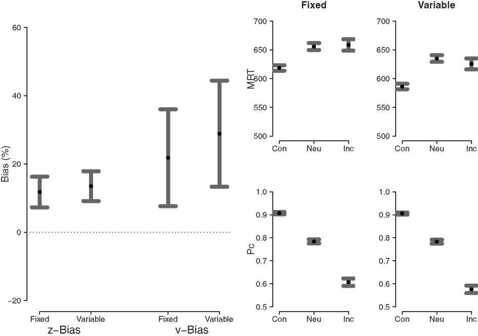
Figure 8. Left panel: starting point bias and drift rate criterion bias. Right four panels: MRT (top) and proportion correct (bottom) for fixed (left) and variable (right) difficulty. Dots represent the mean, error bars represent 95% confidence intervals. Con, consistent; Neu, neutral; Inc, inconsistent.

Since both types of bias are measured on different scales, they cannot be compared directly. The important claim by Hanks et al. (2011) is that bias in the drift rate criterion is larger in the variable difficulty condition than in the fixed difficulty condition. In order to assess this claim we compared both types of bias directly between the two conditions. Consistent with the visual impression from the left panel of Figure 8, the statistical analysis reveal no differences for starting point bias and drift rate criterion bias (t(20) = 0.61, p > 0.05, $p_{H0}^{Bayes}=0.74,$ and t(20) = 0.75, p > 0.05, $p_{H0}^{Bayes}=0.73,$ respectively).

In sum, both in the fixed difficulty condition and in the variable difficulty condition, participants exhibit bias in starting point and drift rate criterion. The results suggest there is no difference between the two conditions in the amount of each type of bias, challenging the claim by Hanks et al. (2011) that bias in the drift rate criterion should be more pronounced when stimulus difficulty is variable than when it is fixed.

Model Predictives

In cognitive modeling, model fit can be assessed by means of model predictives. Model predictives are simulated data generated from the cognitive model, based on the parameter estimates for the real data. If the generated data closely resemble the real empirical data, then the model fit is deemed adequate (e.g., Gelman and Hill, 2007).

For this experiment, we drew 100 samples from the real data set and generated diffusion model parameter estimates for each participant and each condition separately using a bootstrap procedure. For each of these samples, we generated synthetic data, for which we calculated the 0.1, 0.3, 0.5, 0.7, and 0.9 RT quantiles for both the real data set and the synthetic data set. The real and synthetic RT quantiles are shown in Figure 9.

FIGURE 9

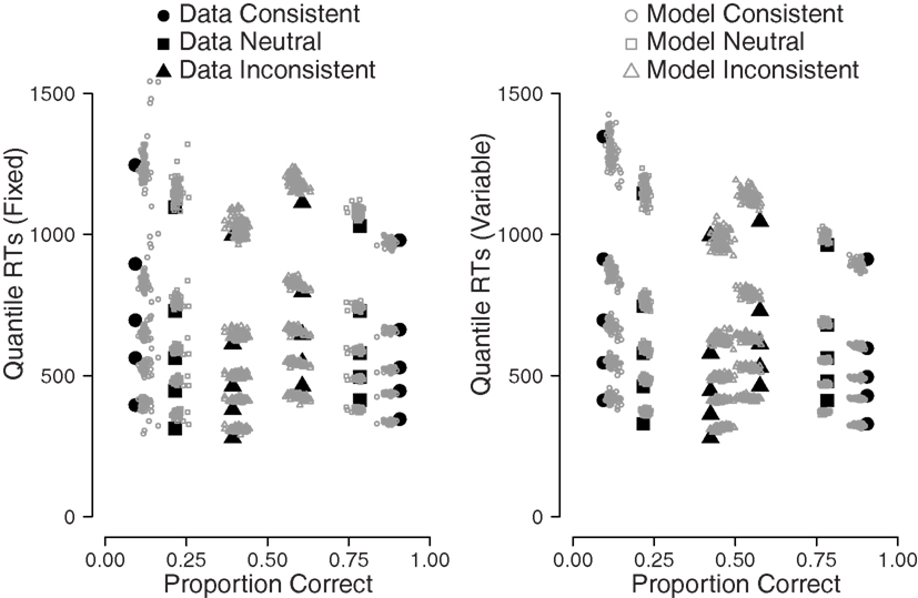
Figure 9. Model predictives indicate that the parameter estimates of DMAT describe the data well. Filled symbols: empirical data. Open symbols: bootstrapped synthetic data, based on the model parameter estimates.

Figure 9 shows a quantile probability plot (e.g., Ratcliff, 2002), where the left-hand side represents error RTs for the five quantiles, and the right-hand side represents correct RTs for those same quantiles. The circles represent stimuli that were consistent with the biased response direction, the squares represent stimuli that were neutral, and the triangles represent stimuli that were inconsistent with the biased response direction. The filled symbols in the figure show the empirical data, the open symbols show the simulated data that were generated using the DMAT parameter estimates.

For response accuracy, the correspondence between the empirical data and the synthetic data can be judged by the horizontal disparity between the data points and the model points. Figure 9 shows that the diffusion model captures the error rate reasonably well for most of the stimulus types, as indicated by the horizontal disparity between the filled and open symbols. The diffusion model does capture the RTs well, as can be judged from the vertical disparity between the filled and open symbols. The quantile probability plot nicely shows how correct responses are fastest for consistent stimuli and slowest for inconsistent stimuli, whereas error responses are fastest for inconsistent stimuli and slowest for consistent stimuli, which is consistent with prior bias (see, e.g., Mulder et al., 2012).

Conclusion

It is not straightforward to perform optimally in response time tasks in which one response option is more likely than the other. When stimulus difficulty is fixed across trials, Edwards (1965) has demonstrated that optimal performance requires advance information to be accommodated solely by a shift in starting point. Recently, Hanks et al. (2011) claimed that when stimulus difficulty varies from trial-to-trial, optimal performance also requires a shift in drift rate criterion (i.e., dynamic bias).

The contribution of this paper is twofold. Firstly, we demonstrated that in theory, optimal performance can be achieved by a shift in starting point only. This result holds regardless of whether stimulus difficulty is fixed or variable from trial-to-trial. Secondly, we presented empirical data showing that people accommodate bias similarly for conditions of fixed and variable across-trial difficulty. Specifically, decision makers incorporate both prior and dynamic bias, and no evidence suggested that the presence of variability in stimulus difficulty made participants rely more on shifts in the drift rate criterion.

In the theoretical part, we first considered the interrogation paradigm. We demonstrated that optimal performance can be achieved by entertaining a bias in starting point, by entertaining a bias in the drift rate criterion, or by a combination of the two. There was no qualitative difference between conditions of fixed and variable across-trial stimulus difficulty.

It could be argued that the theoretical results of the interrogation paradigm are unlikely to apply in practice. Specifically, participants need to know the exact moment of the deadline T to be able to utilize the trade-off between starting point and drift rate criterion. Also, the argument of Hanks et al. (2011) depends on the time course of the decision process: long decisions are most likely difficult decisions, so the longer a decision takes, the more adaptive it becomes to select the biased response alternative. In the interrogation paradigm, however, each decision process takes an identical amount of time.

Another complication when interpreting results for the interrogation paradigm is that for variable difficulty, the optimal setting of the starting point depends on the time deadline (see equation (7)). Because the decision maker does not know the exact value of the time deadline, a more realistic expression should integrate over some unknown distribution of time deadlines that describes the uncertainty in T on the part of the decision maker.

In a task setting without response deadline, our results show that optimal performance is achieved by shifting only the starting point; additionally shifting the drift rate criterion only serves to deteriorate performance. Crucially, we found that this result is true for both fixed and variable across-trial stimulus difficulty. As such, our results conflict with the claim by Hanks et al. (2011) that optimal decision makers should entertain a shift in drift rate criterion to accommodate bias under conditions of variable stimulus difficulty.

In the empirical part, we conducted an experiment in which we manipulated across-trial stimulus difficulty in order to investigate if performance of decision makers is optimal. We also wanted to test whether decision makers accommodate bias differently in decision environments with fixed and variable across-trial stimulus difficulty. We successfully manipulated across-trial variability in difficulty, as evidenced by a higher value of across-trial drift rate variability η for variable across-trial difficulty than for fixed-trial difficulty. Our results showed that performance of participants was not optimal: decision makers implemented both a shift in starting point and a shift in drift rate criterion in order to deal with bias in prior information about the decision alternatives. Contrary to the theory of Hanks et al. (2011), there was no difference in the implementation of dynamic bias between conditions of fixed and variable across-trial stimulus difficulty.

In sum, we conclude that dynamic bias is not needed for optimal performance, not when stimulus difficulty is fixed and not when it is variable. From the perspective of optimality, advance information should affect only prior bias (i.e., starting point), such that the evidence threshold is lowered for the choice alternative that is most likely to be correct a priori. In practice it appears that people use both prior bias and dynamic bias; our experiment suggests that increasing the variability of stimulus difficulty does not cause participants to accommodate advance information preferentially by shifting the drift rate criterion.

Conflict of Interest Statement

The authors declare that the research was conducted in the absence of any commercial or financial relationships that could be construed as a potential conflict of interest.

Acknowledgments

This research was supported by a Vidi grant from the Netherlands Organisation for Scientific Research (NWO). This paper is part of the Research Priority Program Brain and Cognition at the University of Amsterdam. We thank Anja Sommavilla for testing the participants. This publication was supported by an Open Access grant from the Netherlands Organisation for Scientific Research (NWO).

Footnotes

1. ^Parameter s is a scaling parameter that is usually fixed. For the remainder of this paper, we set it to 0.1.
2. ^This is commonly the case in perceptual decision tasks, such as the random dot motion task (Newsome et al., 1989), which we will be using in the experiment reported below.
3. ^Note that for an unbiased decision, z = 0.
4. ^Note that for an unbiased decision, z = a/2.
5. ^For the remainder of this article we set non-decision time T_er = 0.
6. ^We explored a range of values for Bias β, accuracy, and drift rate. The results were always qualitatively similar: the lowest MRT was achieved when v_c = 0.
7. ^In theory, negative drift rates could lead to a larger bias. However, none of our participants had negative drift rates for any of the stimulus types.
8. ^Note that the alternative hypothesis is roughly twice as likely as the null-hypothesis according to $p_{H0}^{Bayes}.$

References

Bogacz, R., Brown, E., Moehlis, J., Holmes, P., and Cohen, J. D. (2006). The physics of optimal decision making: a formal analysis of models of performance in two-alternative forced choice tasks. Psychol. Rev. 113, 700–765.

Pubmed Abstract | Pubmed Full Text | CrossRef Full Text

Brainard, D. H. (1997). The psychophysics toolbox. Spat. Vis. 10, 433–436.

Pubmed Abstract | Pubmed Full Text | CrossRef Full Text

Britten, K. H., Shadlen, M. N., Newsome, W. T., and Movshon, J. A. (1992). The analysis of visual motion: a comparison of neuronal and psychophysical performance. J. Neurosci. 12, 4745–4765.

Pubmed Abstract | Pubmed Full Text

Diederich, A., and Busemeyer, J. R. (2006). Modeling the effects of payoff on response bias in a perceptual discrimination task: bound-change, drift-rate-change, or two-stage-processing hypothesis. Percept. Psychophys. 68, 194–207.

Pubmed Abstract | Pubmed Full Text | CrossRef Full Text

Edwards, W. (1965). Optimal strategies for seeking information: models for statistics, choice reaction times, and human information processing. J. Math. Psychol. 2, 312–329.

CrossRef Full Text

Feng, S., Holmes, P., Rorie, A., and Newsome, W. T. (2009). Can monkeys choose optimally when faced with noisy stimuli and unequal rewards? PLoS Comput. Biol. 5, e1000284. doi: 10.1371/journal.pcbi.1000284

Pubmed Abstract | Pubmed Full Text | CrossRef Full Text

Gao, J., Tortell, R., and McClelland, J. L. (2011). Dynamic integration of reward and stimulus information in perceptual decision-making. PLoS ONE 6, e16749. doi: 10.1371/journal.pone.0016749

CrossRef Full Text

Gelman, A., Carlin, J. B., Stern, H. S., and Rubin, D. B. (2004). Bayesian Data Analysis, 2nd Edn. Boca Raton, FL: Chapman and Hall/CRC.

Gelman, A., and Hill, J. (2007). Data Analysis Using Regression and Multilevel/Hierarchical Models. Cambridge: Cambridge University Press.

Gold, J. I., and Shadlen, M. N. (2003). The influence of behavioral context on the representation of a perceptual decision in developing oculomotor commands. J. Neurosci. 23, 632–651.

Pubmed Abstract | Pubmed Full Text

Grasman, R. P. P. P., Wagenmakers, E.-J., and van der Maas, H. L. J. (2009). On the mean and variance of response times under the diffusion model with an application to parameter estimation. J. Math. Psychol. 53, 55–68.

CrossRef Full Text

Hanks, T. D., Mazurek, M. E., Kiani, R., Hopp, E., and Shadlen, M. N. (2011). Elapsed decision time affects the weighting of prior probability in a perceptual decision task. J. Neurosci. 31, 6339–6352.

Pubmed Abstract | Pubmed Full Text | CrossRef Full Text

Laming, D. R. J. (1968). Information Theory of Choice-Reaction Times. London: Academic Press.

Luce, R. D. (1986). Response Times. New York: Oxford University Press.

Mathworks. (1984). Matlab. Available at: http://www.mathworks.com/products/matlab

Mulder, M. J., Bos, D., Weusten, J. M. H., van Belle, J., van Dijk, S. C., Simen, P., van Engeland, H., and Durston, S. (2010). Basic impairments in regulating the speed-accuracy tradeoff predict symptoms of attention-deficit/hyperactivity disorder. Biol. Psychiatry 68, 1114–1119.

Pubmed Abstract | Pubmed Full Text | CrossRef Full Text

Mulder, M. J., Wagenmakers, E. -J., Ratcliff, R., Boekel, W., and Forstmann, B. U. (2012). Bias in the brain: a diffusion model analysis of prior probability and potential payoff. J. Neurosci. 32, 2335–2343.

Pubmed Abstract | Pubmed Full Text | CrossRef Full Text

Newsome, W. T., Britten, K. H., and Movshon, J. A. (1989). Neuronal correlates of a perceptual decision. Nature 341, 52–54.

Pubmed Abstract | Pubmed Full Text | CrossRef Full Text

Newsome, W. T., and Paré, E. B. (1988). A selective impairment of motion perception following lesions of the middle temporal visual area (MT). J. Neurosci. 8, 2201–2211.

Pubmed Abstract | Pubmed Full Text

Palmer, J., Huk, A. C., and Shadlen, M. N. (2005). The effect of stimulus strength on the speed and accuracy of a perceptual decision. J. Vis. 5, 376–404.

Pubmed Abstract | Pubmed Full Text | CrossRef Full Text

Ratcliff, R. (1978). A theory of memory retrieval. Psychol. Rev. 85, 59–108.

CrossRef Full Text

Ratcliff, R. (1985). Theoretical interpretations of the speed and accuracy of positive and negative responses. Psychol. Rev. 92, 212–225.

Pubmed Abstract | Pubmed Full Text | CrossRef Full Text

Ratcliff, R. (2002). A diffusion model account of response time and accuracy in a brightness discrimination task: fitting real data and failing to fit fake but plausible data. Psychon. Bull. Rev. 9, 278–291.

Pubmed Abstract | Pubmed Full Text | CrossRef Full Text

Ratcliff, R., and McKoon, G. (2008). The diffusion decision model: theory and data for two-choice decision tasks. Neural Comput. 20, 873–922.

Pubmed Abstract | Pubmed Full Text | CrossRef Full Text

Ratcliff, R., and Rouder, J. N. (2000). A diffusion model account of masking in two-choice letter identification. J. Exp. Psychol. Hum. Percept. Perform. 26, 127–140.

Pubmed Abstract | Pubmed Full Text | CrossRef Full Text

Ratcliff, R., and Tuerlinckx, F. (2002). Estimating parameters of the diffusion model: approaches to dealing with contaminant reaction times and parameter variability. Psychon. Bull. Rev. 9, 438–481.

Pubmed Abstract | Pubmed Full Text | CrossRef Full Text

Rorie, A. E., Gao, J., McClelland, J. L., and Newsome, W. T. (2010). Integration of sensory and reward information during perceptual decision-making in lateral intraparietal cortex (LIP) of the macaque monkey. PLoS ONE 5, e9308. doi: 10.1371/journal.pone.0009308

CrossRef Full Text

Rouder, J. N., Speckman, P. L., Sun, D., Morey, R. D., and Iverson, G. (2009). Bayesian t-tests for accepting and rejecting the null hypothesis. Psychon. Bull. Rev. 16, 225–237.

Pubmed Abstract | Pubmed Full Text | CrossRef Full Text

Simen, P., Contreras, D., Buck, C., Hu, P., Holmes, P., and Cohen, J. D. (2009). Reward rate optimization in two-alternative decision making: empirical tests of theoretical predictions. J. Exp. Psychol. Hum. Percept. Perform. 35, 1865–1897.

Pubmed Abstract | Pubmed Full Text | CrossRef Full Text

van Ravenzwaaij, D., Brown, S., and Wagenmakers, E.-J. (2011). An integrated perspective on the relation between response speed and intelligence. Cognition 119, 381–393.

Pubmed Abstract | Pubmed Full Text | CrossRef Full Text

van Ravenzwaaij, D., van der Maas, H. L. J., and Wagenmakers, E. -J. (2012). Optimal decision making in neural inhibition models. Psychol. Rev. 119, 201–215.

Pubmed Abstract | Pubmed Full Text | CrossRef Full Text

Vandekerckhove, J., and Tuerlinckx, F. (2007). Fitting the Ratcliff diffusion model to experimental data. Psychon. Bull. Rev. 14, 1011–1026.

Pubmed Abstract | Pubmed Full Text | CrossRef Full Text

Wagenmakers, E.-J. (2007). A practical solution to the pervasive problems of p-values. Psychon. Bull. Rev. 14, 779–804.

Pubmed Abstract | Pubmed Full Text | CrossRef Full Text

Wagenmakers, E.-J. (2009). Methodological and empirical developments for the Ratcliff diffusion model of response times and accuracy. Eur. J. Cogn. Psychol. 21, 641–671.

CrossRef Full Text

Wagenmakers, E.-J., van der Maas, H. J. L., and Grasman, R. P. P. P. (2007). An EZ-diffusion model for response time and accuracy. Psychon. Bull. Rev. 14, 3–22.

Pubmed Abstract | Pubmed Full Text | CrossRef Full Text

Wald, A., and Wolfowitz, J. (1948). Optimal character of the sequential probability ratio test. Ann. Math. Stat. 19, 326–339.

CrossRef Full Text

Yang, T., Hanks, T. D., Mazurek, M., McKinley, M., Palmer, J., and Shadlen, M. N. (2005). “Incorporating prior probability into decision-making in the face of uncertain reliability of evidence,” in Poster Presented at the Meeting of the Society for Neuroscience, Washington, DC.

Appendix

Derivation of Equation (6)

To understand the derivation of equation (6) from equation (5), let us focus on the first part $\Phi \left[\frac{\left(\xi +v_c\right)T+z}{s\sqrt{T}}\right]$ (the treatment of the second part is analogous) and write it as Φ[Aξ + B], with $A=\frac{\sqrt{T}}{s}$ and $B=\frac{v_{c}T+z}{s\sqrt{T}}$. We then have the following integral I:

$I={\int }_{-\infty }^{+\infty }\Phi \left[A\xi +B\right]\varphi \left(\xi ;v,{\eta }^2\right)d\xi ,$

where ϕ(ξ; v, η²) stands for the normal density function for ξ with mean v and variance η². We can continue as follows:

$\begin{array}{l}I={\int }_{-\infty }^{+\infty }\Phi \left[A\xi +B\right]\varphi \left(\xi ;v,{\eta }^2\right)d\xi \\ ={\int }_{-\infty }^{+\infty }{\int }_{-\infty }^{A\xi +B}\varphi \left(x;0,1\right)dx\varphi \left(\xi ;v,{\eta }^2\right)d\xi \\ ={\int }_{-\infty }^{+\infty }{\int }_{-\infty }^B\varphi \left(x;-A\xi ,1\right)\varphi \left(\xi ;v,{\eta }^2\right)dxd\xi \\ ={\int }_{-\infty }^{+\infty }{\int }_{-\infty }^{B∕A}\varphi \left(x;-\xi ,1∕A^2\right)\varphi \left(\xi ;v,{\eta }^2\right)dxd\xi \\ ={\int }_{-\infty }^{B∕A}{\int }_{-\infty }^{+\infty }\varphi \left(x;-\xi ,1∕A^2\right)\varphi \left(\xi ;v,{\eta }^2\right)d\xi dx.\end{array}$

The inner integral is a known integral in Bayesian statistics (see, e.g., Gelman et al., 2004). The kernel of the product of the two normal distributions contains an exponent with quadratic terms in ξ and x (Gelman et al., 2004). Thus, ξ and x have a bivariate normal distribution and thus marginalizing over ξ results in a normal distribution for x.

Using the double expectation theorem (see Gelman et al., 2004), we can find the marginal mean of x:

$E\left(x\right)=E\left[E\left(x|\xi \right)\right]=E\left[-\xi \right]=-v.$

Applying a similar theorem for the marginal variance of x gives (Gelman et al., 2004):

$\text{Var}\left(x\right)=E\left[\text{Var}\left(x|\xi \right)\right]+\text{Var}\left[E\left(x|\xi \right)\right]=E\left[1∕A^2\right]+\text{Var}\left(-\xi \right)=1∕A^2+{\eta }^2.$

Therefore, we can simplify the inner integral to ϕ(x; − v, 1/A² + η²):

$\begin{array}{l}I={\displaystyle {\int }_{-\infty }^{B/A}\varphi \left(x;-v,1/A^2+{\eta }^2\right)dx}\\ ={\displaystyle {\int }_{-\infty }^{\frac{B/A+v}{\sqrt{1/A^2+{\eta }^2}}}\varphi \left(x;0,1\right)}dx\\ =\Phi \left[\frac{B/A+v}{\sqrt{1/A^2+{\eta }^2}}\right]\\ =\Phi \left[\frac{\frac{v_{c}T+z}{T}+v}{\sqrt{s^2/T+{\eta }^2}}\right]\\ =\Phi \left[\frac{\left(v_c+v\right)T+z}{\sqrt[s]{T+T^2{\eta }^2/s^2}}\right],\end{array}$

which is, after multiplication with β, equal to the first term of equation (6). The second part can be found in a similar way.