
- Department of Psychology and Center for Neural Science, New York University, New York, NY, USA
In decision from experience, the source of probability information affects how probability is distorted in the decision task. Understanding how and why probability is distorted is a key issue in understanding the peculiar character of experience-based decision. We consider how probability information is used not just in decision-making but also in a wide variety of cognitive, perceptual, and motor tasks. Very similar patterns of distortion of probability/frequency information have been found in visual frequency estimation, frequency estimation based on memory, signal detection theory, and in the use of probability information in decision-making under risk and uncertainty. We show that distortion of probability in all cases is well captured as linear transformations of the log odds of frequency and/or probability, a model with a slope parameter, and an intercept parameter. We then consider how task and experience influence these two parameters and the resulting distortion of probability. We review how the probability distortions change in systematic ways with task and report three experiments on frequency distortion where the distortions change systematically in the same task. We found that the slope of frequency distortions decreases with the sample size, which is echoed by findings in decision from experience. We review previous models of the representation of uncertainty and find that none can account for the empirical findings.
Estimates of the frequency of events by human observers are typically distorted. In Figure 1A we re-plot data from one of the earliest reports of this phenomenon (Attneave, 1953). Attneave asked participants to estimate the relative frequency of English letters in text and Figure 1A is a plot of their frequency estimates versus actual frequency. Although participants had considerable experience with English text, the estimates were markedly distorted, with the relative frequency of rare letters overestimated, that of common letters, underestimated.
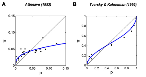
Figure 1. S-shaped distortions of frequency estimates. (A) Estimated relative frequencies of occurrence of English letters in text plotted versus actual relative frequency from Attneave (1953). (B) Subjective probability of winning a gamble (decision weight) plotted versus objective probability from Tversky and Kahneman (1992). R2 denotes the proportion of variance accounted by the fit.
Such S-shaped distortions1 of relative frequency and probability are found in many research areas including decision under risk (for reviews see Gonzalez and Wu, 1999; Luce, 2000), visual perception (Pitz, 1966; Brooke and MacRae, 1977; Varey et al., 1990), memory (Attneave, 1953; Lichtenstein et al., 1978), and movement planning under risk (Wu et al., 2009, 2011).
Figure 1B shows an example from decision under risk (Tversky and Kahneman, 1992). Different participants in the same experiment can have different distortions (Gonzalez and Wu, 1999; Luce, 2000) and a single participant can exhibit different distortion patterns in different tasks (Brooke and MacRae, 1977; Wu et al., 2009) or in different conditions of a single task (Tversky and Kahneman, 1992). We currently do not know what controls probability distortion or why it varies as it does. Gonzalez and Wu (1999) identified this issue as central to research on decision under risk.
We use a two-parameter family of transformations to characterize the distortions of frequency/probability. This family of distortion functions is defined by the implicit equation,

where p denotes true frequency/probability, π(p) denotes the corresponding distorted frequency/probability estimate and,

is the log odds (Barnard, 1949) or logit function (Berkson, 1944). The transformation is an S-shaped curve (examples shown in both panels of Figure 2).
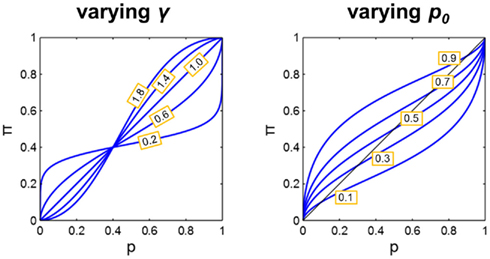
Figure 2. Demonstration of the effects of varying the parameters γ and p0. The parameter p0 in the LLO function is the “fixed point” of the transformation, the value of p which is mapped to itself. The parameter γ, is the slope of the linear transformation on log odds scales, and on linear scales, is the slope of the curve at the crossover point p0. Left: p0 fixed at 0.4 and γ varied between 0.2 and 1.8. Note that the line at γ = 1 overlaps with the diagonal line, i.e., no distortion of probability. Right: γ fixed at 0.6 and p0 varied between 0.1 and 0.9.
The two parameters of the family are readily interpretable. The parameter γ in Eq. 1 is the slope of the linear transformation and the remaining parameter p0 is the “fixed point” of the linear transformation, the value of p which is mapped to itself. To show this, we need only set p = p0 and simplify to get,

Since Lo() is invertible, π(p0) = p0. We refer to p0 as the crossover point.
In Figure 2 we illustrate more generally how the two parameters affect the shape of the distortion function, plotting π against p on linear scales. The transformation maps 0–0, 1–1, and p0 to p0. At point (p0, p0), the slope of the curve equals γ. When γ = 1, π(p) = p, the curve overlaps with the diagonal line, that is, there is no distortion at all. When γ > 1 and 0 < p0 < 1 we see an S-shaped curve. When 0 < γ < 1 and 0 < p0 < 1 we see an inverted-S-shaped curve. When the crossover point p0 is set to either 0 or 1, the curve is no longer S-shaped but simply concave or convex.
This family of functions, with a slightly different parameterization, has been previously used to model frequency distortion (Pitz, 1966). In decision under risk or uncertainty, it has been used to model probability distortion (Goldstein and Einhorn, 1987; Tversky and Fox, 1995; Gonzalez and Wu, 1999). A one-parameter form without the intercept term was first used by Karmarkar (1979) to explain the Allais paradox (Allais, 1953). Following Gonzalez and Wu (1999) we refer to this family of functions as “LLO.”
The LLO function we use is just one family of the functions that can capture the S-shaped transformations. Prelec (1998) proposed another family of functions, which, in most cases, are empirically indistinguishable from the LLO function (Luce, 2000). We return to this point below.
The present paper is organized into four sections. In Section “Ubiquitous Log Odds in Human Judgment and Decision,” we demonstrate good fits of the LLO function to frequency/probability data in a wide variety of experimental tasks. We retrieved data for p and π from tables or figures of published papers and re-plotted them on the log odds scales. The parameters (γ and p0) and goodness-of-fit (R2) of the LLO fit are shown on each plot. We see dramatic differences in γ and p0 across tasks and individuals. We are concerned with two questions: how can we explain the LLO transformation? What determines the slope γ and crossover point p0? We address these two questions in the following sections.
We conducted three experiments to investigate the factors that influence γ and p0. We report them in Section “What Controls the Slope and the Crossover Point?” The task we used was to estimate the relative frequency of a category of symbols in a visual display. We observed systematic distortions of relative frequency consistent with the LLO function and identified several factors that influence γ and p0. We discuss the results in the light of recent findings in decision under risk, especially those in the name of “decision from experience” (Hertwig et al., 2004; Hau et al., 2010).
Although no attempts have been made to explain the various S-shaped distortions of frequency/probability in one theory, there are quite a few accounts for the distortion in one specific task or area. In Section “Previous Accounts of Probability Distortion,” we review these theories or models and contrast them with the empirical findings summarized in Sections “Ubiquitous Log Odds in Human Judgment and Decision” and “What Controls the Slope and the Crossover Point?”
In Section “LLO as the Human Representation of Uncertainty,” we argue that log odds is a fundamental representation of frequency/probability used by the human brain. The LLO transformation in various areas is not coincidence but reflects a common mechanism to deal with uncertainty.
Ubiquitous Log Odds in Human Judgment and Decision
We now demonstrate that the subjective frequency/probability in a wide variety of tasks can be fitted by the LLO function with two parameters γ and p0. In the accompanying figures, we plot subjective frequency/probability versus true frequency/probability on log odds scales. On these scales the LLO function is a straight line with slope γ and crossover point p0. Black dots denote data points. The blue line denotes the LLO fit. When you read the plot, note how different γ and p0 can be for different tasks or individuals. These plots pose quantitative tests for any theory that is aimed at accounting for probability distortions.
Frequency Estimation
We introduced Attneave (1953) earlier as an example of overestimation of small relative frequency and underestimation of large relative frequencies. In his experiment, participants estimated the relative frequency of each letter in written English (Figure 1A). While a linear fit could only account for 63% of the variance, the LLO function fitted to the same data transformed in Figure 3A accounts for 77% of the variance.
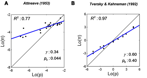
Figure 3. Linear in log odds fits: frequency estimates. The two data sets in Figures 1A,B are re-plotted on log odds scales as (A,B), respectively. The blue line is the best-fitting LLO fit. R2 denotes the proportion of variance accounted by the fit. The S-shaped distortions of frequency/probability on linear scales in Figures 1A,B are well captured by the LLO fits.
Note that the relative frequency of even the most common letter (“e”) is less than 0.15. Intriguingly, the estimated crossover point  0.044, for Attneave’s (1953) data is not far from 1/26 (=0.039), the reciprocal of the number of letters in the alphabet. We return to this point later.
Another impressive example is Lichtenstein et al. (1978). Participants were given a list of 41 possible causes of death in the US, such as flood, homicide, and motor vehicle accidents (MVA). Participants were asked to estimate the frequencies of the causes. The true frequency of one cause was provided to participants as a reference. One group of participants was provided with the frequency of Electrocution (1000) as the reference and a second group, the frequency of MVA (50000). We divided the true frequencies and estimated frequencies (averaged across participants) by the US population (2.05 × 10⁸) to obtain the relative frequencies, p and π. We noticed that although some specific causes were unreasonably overestimated relative to others (e.g., floods were estimated to take more lives than asthma although the latter is nine times more likely), the overestimation or underestimation of relative frequency of all causes as a whole can be satisfactorily accounted by the LLO function. Figure 4A shows the LLO fits for the two groups.
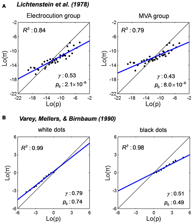
Figure 4. Linear in log odds fits: frequency estimates from memory or perception. Estimated relative frequency is plotted against true relative frequency on log odds scales and fitted by the LLO function. Black dots denote data. The blue line denotes the LLO fit. R2 denotes the proportion of variance accounted by the fit. (A) Estimated frequency of lethal events from Lichtenstein et al. (1978). Participants were asked to estimate the number of occurrences of different causes of death per year in the US. The actual frequency of one cause was provided as a reference for participants to estimate the frequencies of the other causes. The relative estimated and actual frequencies in the plot were the frequencies divided by the then US population. Left: when the frequency of Electrocution (1000) was given as reference. Right: when the frequency of MVA (motor vehicle accident, 50000) was given as reference. (B) Estimated frequency of visual stimuli from Varey et al. (1990). The task was to estimate the relative frequency of black or white dots among a visual array of black and white dots. The proportion of black dots was larger than the proportion of white dots. Two groups of participants respectively estimated the relative frequency of white dots (small p) and black dots (large p). Left: the white dots group (p ≤ 0.5) was estimated. Right: the black dots group (p ≥ 0.5) was estimated.
In the above two examples, participants’ estimation of frequency was based on their memory of events (e.g., reading of a case of lethal events on the newspaper). To show the LLO transformation is not unique to memory nor to sequential presentation of events, our third example is Varey et al. (1990), which demonstrates an LLO transformation in frequency estimation from one visual stimulus. The task was to estimate the relative frequency of either black or white dots among an array of black and white dots. White dots were always less than half of the total number of dots. Eleven levels of relative frequency were used. Participants reported the relative frequency immediately after they saw the visual display. Varey et al. (1990) found considerable distortion of relative frequency. Figure 4B shows the LLO fits separately for participants who estimated the relative frequency of white dots and those who estimated black dots.
Confidence Rating
Confidence rating refers to the task where participants estimate the probability of correctness or success of their own action. For example, in Gigerenzer et al. (1991), participants answered forced-choice questions like “Who was born first? (a) Buddha or (b) Aristotle” and then chose for each question how confident they were to be correct: 50, 51–60, 61–70, 71–80, 81–90, 91–99, or 100% confident. Participants choosing 51–60% were counted to be 55% confident about the answer, and so on. Converted to proportion, the rated confidence is a counterpart of estimated probability, π. The true probability, p, in the confidence rating task is defined as the relative frequency to be correct for a specific choice of confidence level. We re-plot the representative set condition of Gigerenzer et al. (1991) Figure 6 in Figure 5A. The slope γ of the LLO fit is greater than one. That is, an underestimation of small probability (the probability of the harder task) and overestimation of large probability (the probability of the easier task). A qualitative description of this phenomenon is usually referred as a hard–easy effect. This pattern is the reverse of that of the above examples of frequency estimation tasks. We discuss this difference later.
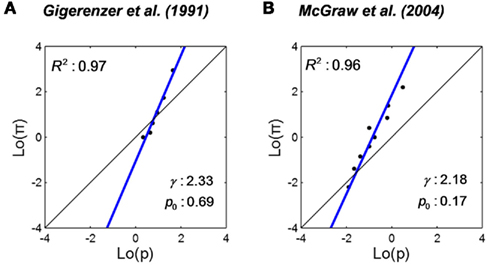
Figure 5. Linear in log odds fits: confidence rating for cognitive and motor responses. Estimated probability of being correct or successful is plotted versus the actual probability on log odds scales and fitted by the LLO function. Black dots denote data. The blue line denotes the LLO fit. R2 denotes the proportion of variance accounted by the fit. (A) Estimated probability of being correct in general-knowledge questions from Gigerenzer et al. (1991). Participants first chose an answer for two alternative general-knowledge questions and then indicated the probability that the answer was correct. (B) Estimated probability of success in basketball shooting from McGraw et al. (2004). Participants rated their probability of success before each basketball shot.
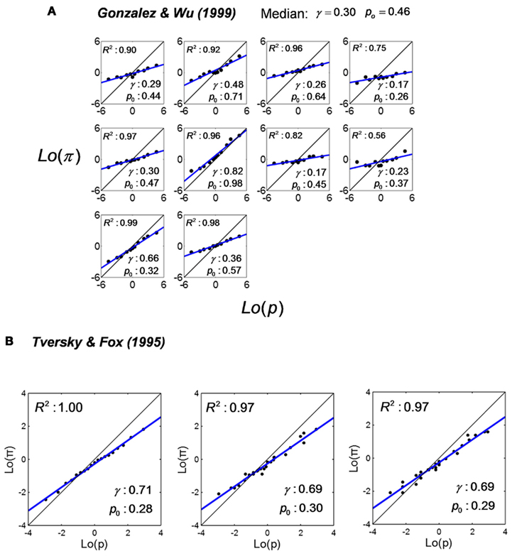
Figure 6. Linear in log odds fits: decision under risk or uncertainty. Decision weight is plotted versus experimenter-stated probability (in decision under risk) or self-judged probability (in decision under uncertainty) and fitted by the LLO function. Black dots denote data. The blue line denotes the LLO fit. R2 denotes the proportion of variance accounted by the fit. (A) Decision weights of individual participants from Gonzalez and Wu (1999). Each panel is for one participant. Participants chose between a two-outcome lottery and a sure reward. The probability of winning the larger reward of the lottery was stated as p. Decision weight, the counterpart of subjective probability π, was inferred from each participant’s choices based on the Cumulative Prospect Theory. Re-plotted from Figure 6 of Gonzalez and Wu (1999). (B) Decision weights from Tversky and Fox (1995). Participants chose between a lottery offering a probability of a reward or otherwise zero and a sure reward. The probability of winning the larger reward of the lottery p was stated (left panel), or estimated by participants themselves as the probability of a specific Super Bowl prospect (middle panel), or as the probability of a specific Dow-Jones prospect (right panel). Decision weight, the counterpart of subjective probability π, was inferred from participants’ choices based on the Cumulative Prospect Theory Re-plotted respectively from Figures 7–9 of Tversky and Fox (1995).
Gigerenzer et al. (1991) is an example of human confidence on a cognitive task. Similar LLO transformations are found in confidence ratings in motor tasks. McGraw et al. (2004) required participants to attempt basketball shots and give a confidence rating before each attempt. Their results are re-plotted as Figure 5B.
Decision under Risk or Uncertainty
A classical task of decision under risk is to choose between two gambles or between one gamble and one sure payoff. Kahneman and Tversky (1979) proposed that the subjective probability used in decision-making, a.k.a. the decision weight function2, is a non-linear function of the probability stated in the gamble.
Based on their choices between different gambles and different sure payoffs, participants’ decision weight (a counterpart of π) for any specific stated probability (p) can be estimated. In Figures 1B and 3B, we re-plot the decision weight for gains of Tversky and Kahneman (1992) against stated probability on linear scales and log odds scales. The LLO fit explains 97% of the variance, with γ = 0.60 and p0 = 0.40.
The data presented in most decision-making studies are averaged across participants. As an exception, Gonzalez and Wu (1999) elicited decision weights for each individual participants. We re-plot their results on log odds scales in Figure 6A. Each panel is for one participant. The large individual differences are impressive. The slope γ ranges from 0.17 to 0.82, with a median of 0.30. The crossover point p0 ranges from 0.26 to 0.98, with a median of 0.46. The only common point across participants seems to be that all the slopes are lesser than one.
When the probabilities of possible consequences of a decision are known, it is decision under risk. When the probabilities are unknown, it is decision under uncertainty. Tversky and Fox (1995) compared probability distortions in decision under risk versus uncertainty. We re-plot their Figures 7–9 on log odds scales in Figure 6B. In the left panel (decision under risk), the probability associated with a gamble, p, was explicitly stated. In the middle and right panels (decision under uncertainty), the probability p was the probability of a specific event in Super Bowl or Dow-Jones and came from participants’ own judgments. Similar probability distortions are revealed in the three panels.
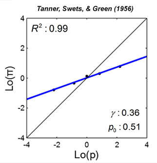
Figure 7. Linear in log odds fit: signal detection theory. Estimated probability of signal present is plotted against the true probability on log odds scales for one participant. Black dots denote data. The blue line denotes the LLO fit. R2 denotes the proportion of variance accounted by the fit. In Tanner et al. (1956), c.f. Green and Swets(1966/1974), participants were asked to report whether a sound signal was present or absent. Estimated probability was inferred from the participant’s decision criterion based on signal detection theory. Data are from Table 4-1 of Green and Swets(1966/1974).
Signal Detection Theory
Signal detection theory (Green and Swets, 1966/1974) is an application of statistical decision theory (Blackwell and Girshick, 1954) to deciding whether a signal is present. In each trial, the observer makes the decision based on her perception of the stimulus. There are four possible outcomes: hit (correctly say “yes” at signal presence), miss (incorrectly say “no” at signal presence), false alarm (FA, incorrectly say “yes” at signal absence), and correct rejection (CR, correctly say “no” at signal absence). If each outcome is associated with a specific payoff and the prior probability of a signal is known, there exists an optimal decision criterion, maximizing expected gain. This decision criterion is determined by the prior probability of signal and the specified rewards.
Based on the relative frequencies of hit, miss, FA, and CR, the actual decision criterion used by the observer can be measured and the experiment can compare the subject’s decision criterion with the optimal criterion. Systematic deviations from the optimal decision criterion have been found in many studies (Green and Swets, 1966/1974; Healy and Kubovy, 1981). It is as if participants overestimate the prior probability when it is small and underestimate the prior probability when it is large.
In Figure 7, we plot Tanner et al.’s (Green and Swets, 1966/1974) data from an auditory signal detection task for one participant on log odds scales. Each data point is obtained from a block of 600 trials with a specific probability of signal present. The straight line is the LLO fit. The slope γ of the probability distortion is 0.36.
In a cognitive signal detection task where participants were asked to classify a number into two categories with different means (Healy and Kubovy, 1981), a similar slope, 0.30, was found.
Summary
At this moment, you are probably intrigued by the same two questions as the authors are: why does probability distortion in so many tasks conform to an LLO transformation? What determines the slope γ and crossover point p0?
The plots we present here reflect only part of the empirical results we have reviewed. To provide a more complete picture, we clarify the following two points.
First, the slope γof the LLO transformation is not determined by the type of task. The slope γ of the same task can be less than one under some conditions and greater than one under others, not to mention the quantitative differences. For example, the typical distortion in relative frequency estimation is an overestimation of small relative frequency and underestimation of large relative frequency, corresponding to γ < 1. But in a visual task that resembles Varey et al. (1990), Brooke and MacRae (1977) found the reverse distortion pattern: an underestimation of small relative frequencies and overestimation of large relative frequencies.
In decision-making under uncertainty, a reversal is reported in Wu et al. (2009), where the probability of a specific outcome is determined by the variance of participants’ own motor errors. The reverse distortion pattern is also implied in a variant of the classical task of decision under risk called “decision from experience” (Hertwig et al., 2004; Ungemach et al., 2009), in which participants acquire the probability of specific outcomes by sampling the environment themselves. We will go into more details in the next section.
Second, the crossover point of the LLO transformation is not determined by the type of task, either. See the difference between Attneave (1953) and Lichtenstein et al. (1978).
Luce (2000, Section 3.4.1–3.4.2) discusses the form of the probability weighting function noting that it is not always S-shaped but can be a simple convex or concave curve. As we noted above, LLO with the crossover point set to 0 or 1 can generate such shapes.
While the LLO family provides good fits to all of the data we have obtained, a two-parameter form of Prelec’s model of the probability weighting function (Prelec, 1998; Luce, 2000, Section 3.4) also provides good fits (not reported here). We concentrate on LLO primarily because of the ready interpretability of its parameters and its links to current work on the neural representation of uncertainty discussed below. As Luce (2000) notes, it is difficult to discriminate competing models of the probability weighting function in decision under risk by their fits to data.
What Controls the Slope and the Crossover Point?
What controls the slope γ and crossover point of the LLO transformation in a specific task? In this section we report three new experiments on frequency/probability distortions.
Gonzalez and Wu (1999) identified some of the factors that make decision under risk a less than ideal paradigm for studying distortions in probability. The most evident is that analysis of data requires simultaneous consideration of probability distortion and valuation of outcomes.
The task we consider here is estimation of the relative frequency of one color of dot among a crowd of two or more colors of dots, a task used by Varey et al. (1990) and other earlier researchers (Stevens and Galanter, 1957). The task is illustrated in the two displays on Figure 8A which consists of 200 (left) or 600 (right) dots placed at random. In both cases, 20% of the dots are black. The observer viewed briefly presented arrays like these and judged the relative frequency of black dots (alternatively, white dots). We varied the true relative frequencies from trial to trial and fit the estimated relative frequencies against the true relative frequencies with the LLO function to obtain γ and p0. We compared γ and p0 across conditions.
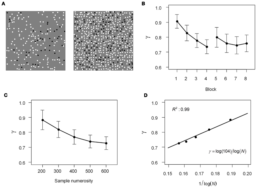
Figure 8. Slope of distortion in relative frequency estimation. The methods and results of Experiment 1. (A) Examples of the relative frequency task: what proportion of the dots are black? The left display contains 200 dots in total, the right, 600. In both displays, 20% of the dots are black. (B) Effect of experience. The mean slope γ across 11 participants is plotted against block index, one to four for the first session, five to eight for the second session. Later blocks are supposed to be associated with more experience. More experience led to greater distortion (γ further from 1). Error bars denote SEs of the mean. (C) Effect of sample numerosity. The slope γ across 11 participants is plotted as a function of sample numerosity N (the total number of dots displayed in a trial). Larger sample numerosity resulted in greater distortion (γ further from 1). Error bars denote SEs of the mean. (D) The function of the mean γ to sample numerosity, N. Dots denote data. Solid line denotes the fit of γ as proportional to the reciprocal of log N.
Experiment 1: Slope
In earlier studies on frequency estimation, some researchers found that small relative frequencies are overestimated and large relative frequencies underestimated (Stevens and Galanter, 1957; Erlick, 1964; Varey et al., 1990) while others found no distortion or even the reverse distortion (Shuford, 1961; Pitz, 1966; Brooke and MacRae, 1977). Different researchers obtained contradictory results even when the task they used was almost the same (e.g., Erlick, 1964; Pitz, 1966). Expressed in the language of LLO, it is a controversy about the slope γ. There is clue in the literature that the numerosity of samples might play a role.
In Experiment 1, participants estimated the relative frequency of either black or white dots among black and white dots. Each participant completed eight blocks. We examined the effects of two factors on γ and p0: experience (block number) and sample numerosity, N, the total number of dots in a trial, which could be 200, 300, 400, 500, or 600.
Methods
Participants. Eleven participants, seven female and four male, participated. Six of them estimated the relative frequency of black dots, the remaining five, white. One additional participant was excluded from the analysis because of marked inaccuracy. All participants gave informed consent and were paid $12/h for their time. The University Committee on activities involving human subjects (UCAIHS) at New York University approved the experiment.
Apparatus and Stimuli. Stimuli were black and white dots displayed on a gray background. They were presented on a SONY GDM-FW900 Trinitron 24″ CRT monitor controlled by a Dell Pentium D Optiplex 745 computer using the Psychophysics Toolbox (Brainard, 1997; Pelli, 1997). A chinrest was used to help maintain a viewing distance of 40 cm. The dots were randomly scattered uniformly within a 17° × 17° area at the center of screen. Each dot had a nominal diameter of 0.26°.
Procedure. On each trial the display of black and white dots was presented for 1.5 s. Participants were asked to estimate the relative frequency of black or white dots. Their estimates were numbers between 1 and 999 interpreted as their estimate of relative frequency out of as 1000. Each participant made estimates for only one color of dots (black or white) and the color assigned to each participant was randomized. Participants were encouraged to be as accurate as possible. No feedback was given.
Trials were organized into blocks of 100 trials. In each block all of the relative frequencies 0.01, 0.02, …, 0.99 except 0.50 occurred once and 0.50 occurred twice. The total number of dots (numerosity, N) in a display could be 200, 300, 400, 500, or 600, with each numerosity occurring in 20 trials of each block. Their order within a block was randomized. Each participant completed two sessions of four blocks on two different days, completing a total of two sessions × four blocks × 100 trials = 800 trials. Before the first block of each session there were five trials of practice.
Results
Effect of experience. The experimental blocks were numbered from 1 to 8 in order. We refer to block index as experience. We fitted the estimated relative frequency to Eq. 1 separately for each participant and each block and then averaged the coefficients γ and p0 across the 11 participants.
Starting from slightly less than one, the slope γ became shallower with experience (Figure 8B), dropping by 16% from Block 1 (0.91) to Block 8 (0.76). A repeated-measures ANOVA showed a significant effect of experience on γ, F(7,70) = 5.59, p < 0.0001,  Post hoc analyses using Tukey’s honestly significant difference criterion at 0.05 significance level indicated that Block 1 had a significantly larger γ than all the other blocks except Block 2.
The crossover point p0 fluctuated around 1/2 (0.5) in all the blocks, ranging from 0.42 to 0.55. According to a repeated-measures ANOVA, p0 did not vary significantly across blocks, F(7,70) = 0.69, p = 0.68,  We concluded that experience affected the slope parameter γ but not the crossover point p0.
Effect of sample numerosity. We used a similar procedure to analyze the effect of sample numerosity as we used in the effect of experience above.
As sample numerosity increased, the slope γ declined (Figure 8C). The γ for displays of 600 dots (0.73) was 18% smaller than that of 200 dots (0.88). A repeated-measures ANOVA showed a significant effect of sample numerosity on γ, F(4,40) = 17.71, p < 0.0001,  Post hoc analyses using Tukey’s honestly significant difference criterion at 0.05 significance level indicated significant decline from 200 to all the larger numerosities, and from 300 to 500 and 600.
Moreover, the relationship of γ to N can be best fitted with a function with one-parameter C:

A least-squares fit of Eq. 4 captured 99% of the variance of γ (Figure 8D). The estimate for the parameter C was 104.
The crossover point p0 was 0.50, 0.54, 0.51, 0.68, 0.68, respectively for the numerosity of 200, 300, 400, 500, 600. Similar to experience, the effect of sample numerosity failed to reach significance, F(4,40) = 2.17, p = 0.08,  To conclude, we found that sample numerosity affected the γ but found only a marginally significant effect of sample numerosity on p0.
Experiment 2: Crossover Point
What determines the crossover point p0? In Experiment 1, p0 was around 0.5 and little affected by experience or sample numerosity. But recall that the estimation of the relative frequency of the 26 English letters (Attneave, 1953) ends up with p0 = 0.044, very different from 0.5 and coincidently not far from 1/26. Fox and Rottenstreich, 2003; See et al., 2006) suggested that when there are m categories, the crossover point should be p0 = 1/m.
Experiment 2 was focused on testing the prediction of p0 = 1/m. The results of Experiment 1 were consistent with the prediction where there were two categories of dots, black and white. In Experiment 2, we set m = 4 (participants were asked to estimate the relative frequency of a specific color among four colors of dots).
Methods
Participants. Ten participants, nine female and one male, participated. None had participated in Experiment 1. All reported normal color vision and passed a color counting test. All subjects gave informed consent and were paid $12/h for their time. The UCAIHS at New York University approved the experiment.
Apparatus and stimuli. The same as Experiment 1, except that dots could any of four colors, red, green, white, or black.
Procedure. In each trial a display of black, white, red, and green dots were presented for 3 s. Afterward one of the four colors was randomly chosen and participants were asked to estimate the relative frequency of dots of this specific color. As in Experiment 1, participants input a number between 1 and 999 as the numerator of 1000 and no feedback was given.
In any trial, the relative frequencies of the four colors were multinomial-like random distributions centered at (0.1, 0.2, 0.3, 0.4) and each relative frequency was constrained to be no less than 0.02. The order of relative frequencies for different colors was randomized. The total number of dots in a display could be 400, 500, or 600, each numerosity occurring in 32 trials of a block. Each participant completed one session of five blocks. That is, five blocks × 96 trials = 480 trials in total.
Results
Fox and Rottenstreich, 2003; See et al., 2006) suggested the crossover point of 1/m but reasoned that it is because people are using a “guessing 1/m” when they are totally ignorant of the relative frequency. In our case, because the to-be-estimated color was indicated after the display of dots, there is a good chance participants might fail to encode the color in question.
In an attempt to further test the “guessing 1/m” heuristic, we considered an additional measure. The preferred response of a participant was defined as the value (rounded to the second digit after the decimal point) that the participant used most often in estimation. The actual relative frequencies in all trials were close to uniformly distributed within the range of [0.06, 0.36] and had a much lower density outside. If on some proportion of trials observers defaulted to the fixed prior value 0.25, as suggested by the heuristic, we would expect to find a “spike” in observers’ estimates of relative frequency at that value.
For each participant, we left out the trials whose estimated relative frequencies were within preferred response ± 0.04 and fit the remaining trials to Eq. 1 to get the crossover point.
For the 10 participants, we computed the mean and 95% confidence interval separately for crossover point and for preferred response. The crossover point was 0.22 ± 0.07, indistinguishable from 1/4 (0.25). Note that it was much lower than 0.5. If this were the result of the “guessing 1/4” heuristic, we would expect a positive correlation between crossover point and preferred response. However, no significant correlation was detected, Pearson’s r = 0.29, p = 0.42. Moreover, the preferred response was 0.18 ± 0.06, lower than 1/4 (0.25).
We concluded that the prediction of p0 = 1/m, was supported, but it was unlikely to be the result of the heuristics discussed above.
Experiment 3: Slope and Discriminability
Tversky and Kahneman (1992) and Gonzalez and Wu (1999) conjecture that the shape of the probability weighting function is controlled by the “discriminability” of probabilities. In Experiment 3, we tested the “discriminability hypothesis” for relative visual numerosity judgments. We measured the just noticeable difference (JND) of relative frequency at 0.5 for the five numerosities used in Experiment 1. If the shallower slope for a larger sample numerosity is caused by a lower discriminability (as consistent with the intuition that a larger numerosity makes the estimation task more difficult), we would expect that the JND increases with an increasing numerosity.
Methods
Participants. Ten participants, seven female and three male, participated. None had participated in Experiment 1 or 2. One additional participant was excluded for failing to converge in the adaptive staircase procedures we used to measure JND. All subjects gave informed consent and were paid $12/h for their time. The UCAIHS at New York University approved the experiment.
Apparatus and stimuli. Same as Experiment 1.
Procedure. On each trial two displays of black and white dots were presented, each for 1.5 s, separated by a blank screen of 1 s. Half of the participants judged which display had a higher proportion of black dots, and the other half, white dots.
As in Experiment 1, the total number of dots (numerosity, N) in a display could be 200, 300, 400, 500, or 600. The two displays in a trial always had the same numerosity. To avoid participants comparing the number of black or white dots of the two displays rather than judging the proportion, we jittered the actual numerosity of each display randomly within the range of ±4%.
The proportion of black or white dots of one display was fixed at 0.5. The proportion of the other was adjusted by adaptive staircase procedures. For each of the five numerosity conditions, there was one 1-up/2-down staircase of 100 trials, resulting in 500 trials in total Each staircase had multiplicative step sizes of 0.175, 0.1125, 0.0625, 0.05 log unit, respectively for the first, second, third, and the remaining reversals. The five staircases were interleaved. Five practice trials preceded the formal experiment.
Results
The 1-up/2-down staircase procedure converges to the 70.7% JND threshold. For each participant and numerosity condition, we averaged all the trials after the first two reversals to compute the threshold. The mean threshold across participants was 0.57, 0.57, 0.56, 0.56, 0.55, respectively for the numerosity of 200, 300, 400, 500, 600. According to a repeated-measures ANOVA, there was no significant difference in the JND threshold for different numerosities, F(4,36) = 2.05, p = 0.11,  Differences in discriminability are not responsible for the differences in probability distortion observed in Experiment 1.
Discussion
As demonstrated in Section “Ubiquitous Log Odds in Human Judgment and Decision,” the distortions of relative frequency and/or probability in a variety of judgment and decision tasks are closely approximated by a linear transformation of the log odds with two parameters, the slope γ and crossover point p0 (LLO, the Eq. 1). We investigated in three experiments what determines these two parameters of the distortion of relative visual frequency.
In Experiment 1 we found that slope γ decreased with increasing experience or larger sample numerosity. Intuitively, these trends are surprising, because an accumulation of experience or a larger sample size should reduce “noise” and thus lead to more accurate estimation. Interesting, the slope γ was proportional to the reciprocal of log N. We cannot find a satisfactory explanation for these effects in the literature. However, there is a parallel sample numerosity effect emerging in an area of decision under risk. We explore the implications under the subtitles below.
In both Experiment 1 and 2 we found that the crossover point p0 agrees with a prediction of p0 = 1/m. Our results are consistent with the category effect found in Fox and Rottenstreich, 2003; See et al., 2006), but we also showed that this is unlikely to be due to the “guessing 1/m” heuristic they suggested.
Decisions from experience
Recently, research on decision-making has begun to focus on how the source of probability/frequency information affects probability distortion. This new research area contrasts “decision from experience” (Barron and Erev, 2003; Hertwig et al., 2004; Hadar and Fox, 2009; Ungemach et al., 2009; for review, see Rakow and Newell, 2010), to traditional “decision from description.”
What are the implications of our results for decision from experience? A typical finding in decision from experience is an underweighting of small probabilities (e.g., Hertwig et al., 2004), as opposed to the overweighting of small probabilities in decision from description (Luce, 2000). Several authors (Hertwig et al., 2004; Hadar and Fox, 2009) conjectured that this reversal is due to probability estimates based on small samples. Consistent with their conjecture, Hau et al. (2010) found that the magnitude of underweighting of small probabilities decreased as sample size increased. With a very large sample size, Glaser et al. (in press) even obtained the classical pattern of an overweighting of small probabilities.
In the language of LLO, the larger the numerosity (sample size), the shallower the slope of the probability distortion (underweighting small probabilities corresponds to a slope of over one). Note that this effect of sampling size on the probability distortion in decision from experience qualitatively parallels to what is found in Experiment 1. And according to Eq. 4, the empirical fit we found for γ, when N = C, there would be no probability distortion. We conjecture that for decision from experience, there exists a specific sample size at which there is no distortion of probability.
There is another hint in the literature that the highly ordered changes in probability distortion that we observe in visual numerosity tasks would also show up in decision-making tasks where probability information is presented as visual numerosity. Denes-Raj and Epstein (1994) asked participants to choose between two bowls filled with jelly beans, one large (100 jelly beans) and one small (10 jelly beans). Participants were explicitly told the proportion of winning jellybeans in both bowls by the experimenters but they still showed a strong preference for the large bowl with 60% of participants choosing a large bowl with 9/100 winning jellybeans over a small bowl with 1/10 winning jellybeans. This outcome suggests an effect of numerosity qualitatively consistent with our results.
We have also shown that we can systematically manipulate the crossover point p0 in a relative visual numerosity task. The crossover point is often assumed not to vary in decision-making under risk (Tversky and Kahneman, 1992; Tversky and Fox, 1995; Prelec, 1998). Our results lead to the conjecture that, in decisions with relative frequency signaled by displays with m > 2 categories, the crossover point will vary systematically.
Confidence ratings
Gigerenzer (Gigerenzer et al., 1991; Gigerenzer, 1994) distinguished between human reasoning about single-event probability and frequency. When asked to rate their confidence about one event, people’s default response was to treat the event as a special one that never occurred before and will never occur after, rather than to group the event into a category of events whose frequency is observable.
Probability distortion in confidence rating typically has a slope of γ > 1 (see Figure 5), as reversed to the typical pattern in frequency estimation and decision-making. We conjecture this to be a special case of the sample numerosity effect. That is, γ > 1 when the sample numerosity is very small. It was as if people treat the to-be-rated action as a single-event and sampled very few previous events to making the confidence rating.
Previous Accounts of Probability Distortion
Why do humans distort frequency/probability in the ways that they do? The subjective probability may deviate from the true probability for many reasons, but no simple reason can explain the S-shaped patterns we have observed.
For example, people might overestimate the frequencies of the events that attract more media exposure (Lichtenstein et al., 1978) or are just more accessible to memory retrieval (Tversky and Kahneman, 1974). But this would not cause a patterned distortion of all events. People might be risk-averse in order to maximize biological utility (Real, 1991), or just be irrationally risk-seeking, but neither risk-averse nor risk-seeking tendencies could explain the coexistence of overestimation and underestimation of probabilities.
The S-shaped distortion has received much attention in quite a few areas. Theories and models have been developed to account for the S-shaped distortion in a specific area, although little efforts have been made to build a unified theory for all the areas. In this section, we briefly describe the representative theories and models, organizing them by area. Their predictions, quantitative or qualitative, on slope, and crossover point of the distortion are compared with the empirical results we summarized in Sections “Ubiquitous Log Odds in Human Judgment and Decision” and “What Controls the Slope and the Crossover Point?”
Frequency Estimation
Power models
Spence’s (1990) power model and Hollands and Dyre’s (2000) extension of it, the cyclical power model, are intended to explain the S-shaped patterned distortion in proportion judgment. Proportion here refers to the ratio of the magnitude of a smaller stimulus to the magnitude of a larger one on a specific physical scale, such as length, weight, time, and numerosity. Relative frequency can be regarded as the proportion of numerosity.
The basic assumption is Stevens’ power law: the perceived magnitude of a physical magnitude, such as the number of black dots in a visual array of different colors of dots, is a power function of the physical magnitude with a specific exponential. We apply the power assumption to the estimation of relative frequency as below. Suppose among N dots, there are n1 black dots and n2 other colors of dots. The perceived numerosity would be  and
and  respectively. Accordingly, the estimated relative frequency of black dots is:

Dividing both the numerator and denominator of the right side by Nα, we get the perceived relative frequency as a function of the true relative frequencies:
It is easy to see this is a variant of LLO (substitute Eq. 6 into Eq. 1) which predicts γ = α and p0 = 0.5. Thus an S-shaped distortion follows the assumption of Stevens’ power law.
Hollands and Dyre (2000) assumed that the slope of the distortion of the proportion of a specific physical magnitude depends on the Stevens exponent of the physical magnitude. For instance, length, area, and volume have different Stevens exponential but the exponent of each of them is fixed. This prediction has some difficulties in applying to the estimation of relative frequency. The experiment we reported in Section “What Controls the Slope and the Crossover Point?” would imply that the exponent is not fixed and changes systematically with the total numerosity.
As to the crossover point, Hollands and Dyre (2000) treated it as an arbitrary value, depending on the reference point available to the observer at the time of judgment. This is not consistent with our observation that p0 = 1/m, where m is the number of categories.
Support theory
Tversky et al.’s support theory (Tversky and Koehler, 1994; Rottenstreich and Tversky, 1997) concerns how humans estimate the probability of specific events. The term degree of support refers to the strength of evidence for a hypothesis. The estimated probability of an event is the degree of support for the presence of the event divided by the sum of the degrees of support for the presence and absence of the event.
To explain the inverted-S-shaped distortion of relative frequency, Fox and Rottenstreich, 2003; See et al., 2006) added two assumptions to support theory. First, they assumed that the original degree of support for both the presence and absence of an event are proportional to the corresponding frequencies. Second, before transforming the degree of support into probability, the log odds of degree of support is linearly combined with a prior log odds and the coefficients of the two add up to 1. Following these two assumptions, the resulting estimated probability has the same form as the LLO function.
The value of the prior probability was the crossover point. Fox and Rottenstreich, 2003; See et al., 2006) called this prior the ignorance prior, echoing the human tendency for equal division when in total ignorance of probability information. It follows that p0 = 1/m.
However, the weighted addition of a true log odds and a prior log odds would lead to a γ never greater than 1, unless the prior log odds has a negative weight. Therefore, it cannot explain the γ > 1 cases (Shuford, 1961; Pitz, 1966; Brooke and MacRae, 1977).
The slope of the distortion equals the weight assigned to the true log odds in the combination. Fox and Rottenstreich, 2003; See et al., 2006) suggested that it is positively correlated with the confidence level of the individual who makes the estimation. We consider next model of the distortion of confidence ratings.
Confidence Ratings
Calibration model
The calibration model of Smith and Ferrell (1983) attributes the probability distortion in confidence rating to a misperception of one’s ability to discriminate between correct and incorrect answers, or between successful and unsuccessful actions.
The calibration model borrows the framework of signal detection theory. Correctness and wrongness of an answer, or success and failure of an action, are considered as two alternative states, i.e., signal present and absent. The observer’s confidence, is assumed to be have a constant mapping to the perceived likelihood ratio of the two states. If the discriminability between the two states is perceived to be larger than the true value, small probabilities would be underestimated and large probabilities overestimated, amounting to γ > 1 (as in Figure 5). If the discriminability were underestimated, the reverse pattern would show up.
The calibration model does not necessarily lead to an LLO transformation and does not have any specific predictions for the selection of slope and crossover point.
Stochastic model
Erev et al., 1994; Wallsten et al., 1997) propose that the over- and under-confidence observed in confidence ratings are caused by stochastic error in response. They assume that at a specific time for a specific event, the participant experiences a degree of confidence and translates this experience into an overt report of confidence level by a response rule. The experienced degree of confidence is the log odds of the true judgment plus a random error drawn from a Gaussian distribution. The larger the variance of the random error, the greater the slope of probability distortion deviates from one.
With some specific response rules, the S-shaped distortion can be produced. The predictions of the stochastic model are not intuitive and are illustrated in their computational simulation. One of the predictions states that the underestimation of small probability and overestimation of large probability (i.e., the γ > 1 pattern) widely identified in confidence rating tasks, a seemingly reverse pattern of regression-to-the-mean, is actually a kind of regression-to-the-mean phenomenon disguised by the way how the true probability is defined. The true probability in the confidence rating task is usually defined as the actual success rate of a specific confidence level. That is, successful and unsuccessful actions are grouped by participants’ confidence rating. Wallsten et al. (1997) re-analyzed previous empirical studies and show that if, instead, the true probability of success is computed for each action as an average across participants, the γ > 1 pattern would be obtained.
However, we doubt this effect of true probability definition can apply to the confidence rating data of McGraw et al. (2004), in which the γ > 1 pattern holds even when the success rate of basketball shot is grouped by the distance to the basket rather than by participants’ confidence rating (not shown in Figure 5B).
Decision under Risk or Uncertainty
Adaptive probability theory
Martins (2006) proposed an adaptive probability theory model to explain the inverted-S-shaped distortion of probability in decision under risk. The observed distortions, under this account, reflect a misuse of Bayesian reference. In everyday life, people observe the frequency of a specific event in finite samples of events. The observed relative frequency of the event, even in the absence of observation errors, may deviate from the true probability of the event due to the random nature of sampling. To reduce the influence of sampling error, Martin assumes that people introduce a prior sample and combines it with the observed sample by Bayes’ rule. The resulting estimated probability would be a linear combination of the observed frequency and the prior probability, determined by three parameters: the size of the imagined sample n, the frequency of the event in the prior sample a, the frequency of the other events in the prior sample b. But Martins (2006) did not characterize what controls these parameters or motivate the choice of prior. Martins (2006) further argued that, in the experimental condition, in front of a lottery, e.g., a probability of 0.1 to win $100, participants treat the probability stated by the experimenter not as a true probability, but as an observed frequency from an imagined sample. The decision weight was the result of the Bayesian inference for the true probability.
The involvement of a prior could explain why the estimated probabilities shrink toward a center. However, for any specific n, instead of a S-shaped transform, the estimated probability would be a linear function of the observed relative frequency, To overcome this difficulty, Martins (2006) assumes that sample size n changes with the observed relative frequency, greater for extreme probabilities and less for smaller probabilities. Thus, the parameter n is actually not one-parameter and is chosen arbitrarily to make theory conform to data.
Another difficulty that adaptive probability theory encounters is the underweighting of small probability observed in studies of decision from experience (e.g., Hertwig et al., 2004). Although Martins (2006) did not suggest the theory could be applied to decisions where the probability information comes from sampling, there is no obvious reason that people would not make the Bayesian inference with a real sample.
Future Directions
In this article we examined probability distortion in human judgment and the factors that affect it. An evident direction for future research is to develop process-based models of human use of probability and frequency information. The theories and models we reviewed above are among those that use specific cognitive processes to explain the emergency of the S-shaped distortion of probability (other examples include Stewart et al., 2006; Gayer, 2010, to name a few). While a full treatment of them is beyond the scope of the current paper, it would be interesting to see whether any existing process-based models can be modified to account for the changes in slope and crossover point we have summarized.
LLO as the Human Representation of Uncertainty
We conjecture that log odds to be a fundamental representation of frequency/probability used by the human brain. Here are a few pieces of evidence.
People are Less Biased when Responding in Log Odds
Phillips and Edwards (1966) asked participants to estimate the probability of one hypothesis to be correct among two alternative hypotheses. There were two types of bags of poker chips, differing in their proportions of red chips and blue chips. Participants were informed the proportions. They were given random draws from one bag and were asked to estimate the probability of each type of bag the sample came from. Participants responded with devices in the format of probability, log probability, or log odds. Phillips and Edwards found that when responding in log odds, participants had the least deviation from the correct answer.
Similarity Rating amounts to Reading out Log Odds
Maloney and Dal Martello (2006) provided evidence of the involvement of log odds in kinship perception. Participants saw pairs of photos of children faces. The task of one group of participants was to judge for each pair whether the children were siblings or not. The task of the other group was to rate the similarity between the two faces shown in each pair. The similarity rating of a pair proved to be proportional to the log likelihood ratio of the pair to be and not to be sibling (Figure 9A). It is as if participants were reading out the log likelihood ratio when required to rate the similarity of two faces. DeBruine et al. (2009) replicated this result several times using young adult faces (Figure 9B).
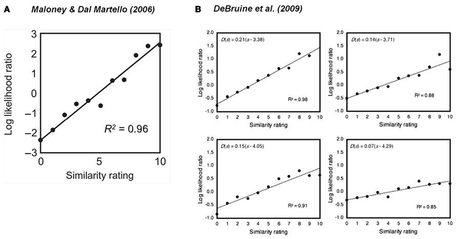
Figure 9. Evidence for log odds as an inherent representation of uncertainty. Participants saw pairs of photos of faces. One group of participants rated the similarity between the two faces in each pair. A second group judged whether the two persons on each pair were related or not. (A) The similarity rating of two children faces is a linear transformation of the log odds of the two children being judged to be related. Reproduced from Maloney and Dal Martello (2006). (B) The similarity rating of two adult faces is a linear transformation of the log odds of the two adults being judged to be related. Reproduced from DeBruine et al. (2009). R2 denotes the proportion of variance accounted by the linear fit. See text for implications.
A plausible Neural Representation of Log Odds
Gold and Shadlen(2001, 2002) propose a computational mechanism for neurons to represent the likelihood ratio of one hypothesis against another. Consider the binary decision whether hypothesis h1 or hypothesis h0 is true. Assume there is a pair of sensory neurons: “neuron” and “antineuron.” The firing rate of “neuron,” x, is a random variable whose distribution is conditional on whether h1 or h0 is true. So does the firing rate of “antineuron,” y. The random distribution of y conditional on h1 is the same as the random distribution of x conditional on h0, and vice versa. For many families of random distributions, such as Gaussian, Poisson, and exponential distributions, Gold and Shadlen prove that the log likelihood ratio of h1 to h0, is a linear function of the firing rate differences between “neuron” and “antineuron,” x − y. While Gold and Shadlen were concerned with making a decision between two alternatives, their proposed neural circuit can potentially be taken as a representation of uncertainty of frequency in log odds form. That is, the log odds can be encoded by two neurons as the difference between their firing rates.
Concluding Remarks
Log odds has been independently developed to fit psychophysical data in many areas of perception and cognition over the course of many years. As early as 1884, Peirce and Jastrow (1885) speculated that the degree of confidence participants gave to their sensation difference judgments was proportional to the log odds of their answers being right. Pitz (1966) used the linear log odds function as a convenient way to fit the data of estimated frequency to true frequency.
In the decision area, Karmarkar (1978, 1979) used a one-parameter linear log odds function to model decision weights. Goldstein and Einhorn (1987) modified Karmarkar’s equation to include the intercept parameter, which was followed by later researchers (Tversky and Fox, 1995; Gonzalez and Wu, 1999; Kilka and Weber, 2001).
For signal detection theory, it is a common practice to plot the actual decision criterion against the optimal decision criterion in the log scale (Green and Swets, 1966/1974; Healy and Kubovy, 1981). It amounts to our log odds plot and the observed distortion of probability is referred to as “conservatism.”
We are seeking for a general explanation for the linear transformation of log odds in these various areas. No matter how different these tasks look like, they are connected by the same evolutionary aim: using possibly imperfect probabilistic information to make decisions that lead to the greatest chance of survival. It is therefore surprising, at first glance, that organisms systematically distort probability. It is doubly surprising that the same pattern of distortion (LLO) is found across a wide variety of tasks.
A full explanation of the phenomena just described would require not only that we account for the form of the distortion but also for the large differences in the values of the two parameters across tasks and individuals and the factors that affect parameter settings. The key question that remains is, then, what determines the slope and crossover point of the linear log odds transformation? We found that in one task we could identify experimental factors that controlled both the slope and crossover point of the LLO transformation of perceived relative numerosity. We conjecture that there are factors in each of the domains we considered that are responsible for the particular choice of probability distortion observed. We need only find out what they are.
Conflict of Interest Statement
The authors declare that the research was conducted in the absence of any commercial or financial relationships that could be construed as a potential conflict of interest.
Acknowledgments
This research was supported in part by grant EY019889 from the National Institutes of Health and by the Alexander v. Humboldt Foundation.
Footnotes
- ^We use the term “distortion” to cover transformations in probability or relative frequency implicit in tasks involving probability or relative frequency. We use “S-shaped” to refer to both S-shaped and inverted-S-shaped. Precisely, Attneave’s (1953) case is an inverted-S-shaped distortion.
- ^We use the generic term “probability distortion” to refer to non-linear transformations of probability in different kinds of task. In decision under risk, the term “probability weight function” or “decision weight function” would coincide with what we refer to as probability distortion.
References
Allais, M. (1953). Le comportement de l’homme rationnel devant le risque: Critique des postulats et axiomes de l’école Américaine (The behavior of a rational agent in the face of risk: critique of the postulates and axioms of the American school). Econometrica 21, 503–546.
Attneave, F. (1953). Psychological probability as a function of experienced frequency. J. Exp. Psychol. 46, 81–86.
Barnard, G. A. (1949). Statistical inference. J. R. Stat. Soc. Series B Stat. Methodol. 11, 115–149.
Barron, G., and Erev, I. (2003). Small feedback-based decisions and their limited correspondence to description-based decisions. J. Behav. Decis. Mak. 16, 215–233.
Berkson, J. (1944). Application of the logistic function to bio-assay. J. Am. Stat. Assoc. 39, 357–365.
Blackwell, D., and Girshick, M. A. (1954). Theory of Games and Statistical Decisions. New York: Wiley.
Brooke, J. B., and MacRae, A. W. (1977). Error patterns in the judgment and production of numerical proportions. Percept. Psychophys. 21, 336–340.
DeBruine, L. M., Smith, F. G., Jones, B. C., Roberts, S. C., Petrie, M., and Spector, T. D. (2009). Kin recognition signals in adult faces. Vision Res. 49, 38–43.
Denes-Raj, V., and Epstein, S. (1994). Conflict between intuitive and rational processing: when people behave against their better judgment. J. Pers. Soc. Psychol. 66, 819–829.
Erev, I., Wallsten, T. S., and Budescu, D. V. (1994). Simultaneous over- and underconfidence: the role of error in judgment processes. Psychol. Rev. 101, 519–527.
Erlick, D. E. (1964). Absolute judgments of discrete quantities randomly distributed over time. J. Exp. Psychol. 67, 475–482.
Fox, C. R., and Rottenstreich, Y. (2003). Partition priming in judgment under uncertainty. Psychol. Sci. 14, 195–200.
Gayer, G. (2010). Perception of probabilities in situations of risk: a case based approach. Games Econ. Behav. 68, 130–143.
Gigerenzer, G. (1994). “Why the distinction between single-event probabilities and frequencies is important for psychology and vice versa,” in Subjective Probability, eds G. Wright and P. Ayton (New York: Wiley), 129–161.
Gigerenzer, G., Hoffrage, U., and Kleinbölting, H. (1991). Probabilistic mental models: a Brunswikian theory of confidence. Psychol. Rev. 98, 506–528.
Glaser, C., Trommershäuser, J., Maloney, L. T., and Mamassian, P. (in press). Comparison of distortion of probability information in decision under risk and an equivalent visual task. Psychol. Sci.
Gold, J. I., and Shadlen, M. N. (2001). Neural computations that underlie decisions about sensory stimuli. Trends Cogn. Sci. (Regul. Ed.) 5, 10–16.
Gold, J. I., and Shadlen, M. N. (2002). Banburismus and the brain: decoding the relationship between sensory stimuli, decisions, and reward. Neuron 36, 299–308.
Goldstein, W. M., and Einhorn, H. J. (1987). Expression theory and the preference reversal phenomena. Psychol. Rev. 94, 236–254.
Gonzalez, R., and Wu, G. (1999). On the shape of the probability weighting function. Cogn. Psychol. 38, 129–166.
Green, D. M., and Swets, J. A. (1966/1974). Signal Detection Theory and Psychophysics. New York: Wiley.
Hadar, L., and Fox, C. R. (2009). Information asymmetry in decision from description versus decision from experience. Judgment Decis. Mak. 4, 317–325.
Hau, R., Pleskac, T. J., and Hertwig, R. (2010). Decisions from experience and statistical probabilities: why they trigger different choices than a priori probabilities. J. Behav. Decis. Mak. 23, 48–68.
Healy, A. F., and Kubovy, M. (1981). Probability matching and the formation of conservative decision rules in a numerical analog of signal detection. J. Exp. Psychol. Hum. Learn. Mem. 7, 344–354.
Hertwig, R., Barron, G., Weber, E. U., and Erev, I. (2004). Decisions from experience and the effect of rare events in risky choice. Psychol. Sci. 15, 534–539.
Hollands, J. G., and Dyre, B. P. (2000). Bias in proportion judgments: the cyclical power model. Psychol. Rev. 107, 500–524.
Kahneman, D., and Tversky, A. (1979). Prospect theory: an analysis of decision under risk. Econometrica 47, 263–291.
Karmarkar, U. S. (1978). Subjectively weighted utility: a descriptive extension of the expected utility model. Organ. Behav. Hum. Perform. 21, 61–72.
Karmarkar, U. S. (1979). Subjectively weighted utility and the Allais paradox. Organ. Behav. Hum. Perform. 24, 67–72.
Kilka, M., and Weber, M. (2001). What determines the shape of the probability weighting function under uncertainty? Manage. Sci. 47, 1712–1726.
Lichtenstein, S., Slovic, P., Fischhoff, B., Layman, M., and Combs, B. (1978). Judged frequency of lethal events. J. Exp. Psychol. Hum. Learn. Mem. 4, 551–578.
Luce, R. D. (2000). Utility of Gains and Losses: Measurement-Theoretical and Experimental Approaches. London: Lawrence Erlbaum, 84–108.
Maloney, L. T., and Dal Martello, M. F. (2006). Kin recognition and the perceived facial similarity of children. J. Vis. 6, 1047–1056.
Martins, A. C. R. (2006). Probability biases as Bayesian inference. Judgment Decis. Mak. 1, 108–117.
McGraw, A. P., Mellers, B. A., and Ritov, I. (2004). The affective costs of overconfidence. J. Behav. Decis. Mak. 17, 281–295.
Peirce, C. S., and Jastrow, J. (1885). On small differences of sensation. Mem. Natl. Acad. Sci. 3, 73–83.
Pelli, D. G. (1997). The VideoToolbox software for visual psychophysics: transforming numbers into movies. Spat. Vis. 10, 437–442.
Phillips, L. D., and Edwards, W. (1966). Conservatism in a simple probability inference task. J. Exp. Psychol. 72, 346–354.
Rakow, T., and Newell, B. R. (2010). Degrees of uncertainty: an overview and framework for future research on experience-based choice. J. Behav. Decis. Mak. 23, 1–14.
Real, L. A. (1991). Animal choice behavior and the evolution of cognitive architecture. Science 253, 980–986.
Rottenstreich, Y., and Tversky, A. (1997). Unpacking, repacking, and anchoring: advances in support theory. Psychol. Rev. 104, 406–415.
See, K. E., Fox, C. R., and Rottenstreich, Y. S. (2006). Between ignorance and truth: partition dependence and learning in judgment under uncertainty. J. Exp. Psychol. Learn. Mem. Cogn. 32, 1385–1402.
Shuford, E. H. (1961). Percentage estimation of proportion as a function of element type, exposure time, and task. J. Exp. Psychol. 61, 430–436.
Smith, M., and Ferrell, W. R. (1983). “The effect of base rate on calibration of subjective probability for true-false questions: model and experiment,” in Analysing and Aiding Decision Processes, eds P. Humphreys, O. Svenson, and A. Vari (Amsterdam: North Holland), 469–488.
Spence, I. (1990). Visual psychophysics of simple graphical elements. J. Exp. Psychol. Hum. Percept. Perform. 16, 683–692.
Stevens, S. S., and Galanter, E. H. (1957). Ratio scales and category scales for a dozen perceptual continua. J. Exp. Psychol. 54, 377–411.
Tversky, A., and Kahneman, D. (1974). Judgment under uncertainty: heuristics and biases. Science 185, 1124–1131.
Tversky, A., and Kahneman, D. (1992). Advances in prospect theory: cumulative representation of uncertainty. J. Risk Uncertain. 5, 297–323.
Tversky, A., and Koehler, D. J. (1994). Support theory: a nonextensional representation of subjective probability. Psychol. Rev. 101, 547–567.
Ungemach, C., Chater, N., and Stewart, N. (2009). Are probabilities overweighted or underweighted when rare outcomes are experienced (rarely)? Psychol. Sci. 20, 473–479.
Varey, C. A., Mellers, B. A., and Birnbaum, M. H. (1990). Judgments of proportions. J. Exp. Psychol. Hum. Percept. Perform. 16, 613–625.
Wallsten, T. S., Budescu, D. V., Erev, I., and Diederich, A. (1997). Evaluating and combining subjective probability estimates. J. Behav. Decis. Mak. 10, 243–268.
Wu, S.-W., Delgado, M. R., and Maloney, L. T. (2009). Economic decision-making under risk compared with an equivalent motor task. Proc. Natl. Acad. Sci. U.S.A. 106, 6088–6093.
Keywords: log odds, subjective probability, probability distortion, frequency estimation, decision-making, uncertainty
Citation: Zhang H and Maloney LT (2012) Ubiquitous log odds: a common representation of probability and frequency distortion in perception, action, and cognition. Front. Neurosci. 6:1. doi: 10.3389/fnins.2012.00001
Received: 19 December 2011; Accepted: 02 January 2012;
Published online: 19 January 2012.
Edited by:
Eldad Yechiam, Technion-Israel Institute of Technology, IsraelReviewed by:
Floris P. De Lange, Radboud University Nijmegen, NetherlandsDavide Marchiori, National Chengchi University, Taiwan
Copyright: © 2012 Zhang and Maloney. This is an open-access article distributed under the terms of the Creative Commons Attribution Non Commercial License, which permits non-commercial use, distribution, and reproduction in other forums, provided the original authors and source are credited.
*Correspondence: Hang Zhang, Department of Psychology, New York University, 6 Washington Place, New York, NY 10003, USA. e-mail: hang.zhang@nyu.edu