Piéron's law and optimal behavior in perceptual decision-making

Piéron’s Law is a psychophysical regularity in signal detection tasks that states that mean response times decrease as a power function of stimulus intensity. In this article, we extend Piéron’s Law to perceptual two-choice decision-making tasks, and demonstrate that the law holds as the discriminability between two competing choices is manipulated, even though the stimulus intensity remains constant. This result is consistent with predictions from a Bayesian ideal observer model. The model assumes that in order to respond optimally in a two-choice decision-making task, participants continually update the posterior probability of each response alternative, until the probability of one alternative crosses a criterion value. In addition to predictions for two-choice decision-making tasks, we extend the ideal observer model to predict Piéron’s Law in signal detection tasks. We conclude that Piéron’s Law is a general phenomenon that may be caused by optimality constraints.

Introduction

Cognitive science features several psychophysical laws. These laws are not only inherently interesting, but often they also bring together phenomena that seem unrelated at first sight. One example of a psychophysical law is Piéron’s Law. Piéron’s Law states that mean response times (MRT) decrease as a power law with increasing stimulus intensity I:

Here α and β are scaling parameters that determine the slope of the function and γ is an intercept (Luce, 1986). The specific parameter values differ between application domains.

Originally, Piéron’s Law was formulated as an effect of stimulus intensity (Piéron, 1914). For example, when participants were instructed to press a button as soon as a light was switched on, MRTs were found to follow a power law decrease with increasing luminance of the light. Over the last century, the law has been reported in many different domains, including brightness detection (Piéron, 1914), tone detection (Chocholle, 1940), taste detection of dissolved substances (Bonnet et al., 1999), odor detection (Overbosch et al., 1989), heat detection (Banks, 1973), and the go/no-go task (Jaskowski and Sobieralska, 2004).

In recent years, Piéron’s Law has been found to hold in two-alternative forced choice (2AFC) tasks as well (Pins and Bonnet, 1996; Palmer et al., 2005; Stafford et al., 2011). Similar to the initial studies that reported Piéron’s Law, MRTs were found to decrease as a power law with increasing stimulus intensity, even though the task was not a signal detection task but instead a choice task. For example, Stafford et al. (2011) demonstrate that reaction times in the Stroop color naming task scale according to a power law with the luminance of the color dimension.

These studies raise the question whether Piéron’s Law describes a specific relation between stimulus intensity and MRT or whether Piéron’s Law is related to the more general notion of discriminability in (perceptual) decision-making. Thus, the typical power law decrease in MRT is not only observed with increasing stimulus intensity, but also when a decision becomes increasingly easy. One reason for arguing in favor of this hypothesis is that the typical stimulus detection task that is associated with Piéron’s Law can be thought of as a 2AFC task. The decision that is required is that between providing a response or withholding a response. The stimulus intensity can now be thought of as a factor on the decision difficulty, because a low intensity stimulus discriminates poorly between the two response alternatives (respond or withhold a response).

In this paper we hypothesize that Piéron’s Law extends to the more general notion of stimulus discriminability. We first show data that support that MRTs in a 2AFC task decrease as a power law with increasing discriminability of the choice alternatives. In particular, we show that the relation between MRT and stimulus discriminability is better supported by a power function than by an exponential function. This comparison quantifies the likelihood that stimulus discriminability indeed leads to Piéron-like behavior. The experimental result supports the idea that Piéron’s Law is more broadly applicable than only in stimulus detection paradigms. Next, we discuss how Piéron-like behavior may be a consequence of optimal decision-making. That is, we present a Bayesian ideal observer model (e.g., Brown et al., 2009) and show that it predicts that MRT decreases as the power of the discriminability of the choices increases. Finally, we extend the Bayesian ideal observer model to include stimulus detection behavior, and discuss under what assumptions optimal stimulus detection would lead to Piéron’s Law.

In the process of studying Piéron’s Law in a 2AFC task, we also make a methodological point: Although never explicitly formulated in this way, Piéron’s Law relates stimulus intensity to mean detection time, rather than mean response time. To account for the non-detection related components of the response time, an intercept parameter is added (γ in Equation 1). To study the relation between stimulus discriminability and decision time in the 2AFC paradigm¹, we separately estimate the non-decision time using a more elaborate choice-response time model (the Linear Ballistic Accumulator model, Brown and Heathcote, 2008). For comparison, we also include the analysis without this additional procedure, and show how this leads to different – implausible – results.

Experiment 1: Stimulus Discriminability in the RDM Task

A 2AFC task that is perfectly suited to address the question at hand is the random-dot motion task (RDM, Ball and Sekuler, 1982; Britten et al., 1992; Salzman and Newsome, 1994; Shadlen and Newsome, 2001; Churchland et al., 2008; Forstmann et al., 2008, 2010a,b; Niwa and Ditterich, 2008; Ho et al., 2009; Mulder et al., 2010; Van Maanen et al., 2011). In this task participants are required to indicate the apparent direction of motion of a cloud of dots that is presented on a computer screen. Typically, a percentage of the dots moves in a designated direction (the target direction), while the remaining dots move randomly. The choice alternatives are presented on a fixed distance from the center of the dot cloud, and their similarity can be manipulated by changing the angular distance between the alternatives, as in Figure 1.

FIGURE 1

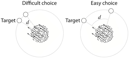
Figure 1. RDM stimulus display. A proportion of the dots move in a target direction indicated by the arrows, while the remaining dots move randomly. The discriminability of the target is manipulated by changing the angular distance (d) between the alternatives.

In Experiment 1, participants were asked to make a choice between two alternative directions of motion. We manipulated the angular distance between the response alternatives to operationalize choice difficulty. Response alternatives that were in close spatial proximity were hypothesized to be hard to discriminate. Response alternatives that were not in close spatial proximity were hypothesized to be easy to discriminate (Figure 1). Note that in this experiment we do not manipulate stimulus intensity, as the dot cloud remains the same in all conditions. Therefore, evidence for a power curve in this experiment would support the hypothesis that Piéron’s Law is a general relation between MRT and stimulus discriminability.

Methods

Participants

Six students (three female, age range 18–20) from the University of Amsterdam participated for course credit. All had normal or corrected-to-normal vision.

Random-dot motion stimulus

To create the moving-dot kinematogram we used the Variable Coherence Random-Dot Motion (VCRDM) library for Psychtoolbox in Matlab (Brainard, 1997)². The appearance of motion in VCRDM is created by controlling the location of a subset of dots for three frames in a row. That is, when the second frame is drawn, the location of a subset of dots will be recomputed to align with the target direction. The location of the remaining dots is randomly assigned. The size of the subset –often referred to as the coherence level – is under the experimenter’s control. We set the coherence at 25%. Pilot studies with several levels of coherence indicated that at a coherence of 25% participants performed above chance for the hardest conditions, whereas they performed below ceiling at the easiest conditions. Each dot consisted of three by three pixels, and the initial locations of each dot sequence were uniformly distributed in an aperture of 5 visual degrees diameter.

Design and procedure

Participants were instructed to indicate the apparent direction of motion of the random-dot kinematogram. The two-choice alternatives were represented by two circles (one blue, one yellow) that were located at 5 visual degrees from the center of the aperture. If the direction of motion was toward the blue alternative, the participants were required to press “z”; if the direction of motion was toward the yellow alternative they were required to press “m.” The location of the alternatives was randomized over the top half of the imaginary circle. However, the blue alternative always remained to the left of the yellow alternative. Therefore, the “z” and “m” response mapping was always congruent with the target positions on the screen. The angular distances between the alternatives were exponentially distributed, to maximize the probability of diverging model fits. Consecutively, the angular distances were 11.5°, 16°, 22.5°, 32°, 45°, 64°, or 90°. The presentation order of the different angular distances was pseudo-randomized in such a way that there were never more than two consecutive trials with the same angular distance between the alternatives.

After a short training session with 14 trials (2 for each angle) the experiment was presented in seven blocks of 210 trials each. After each block, the participant could take a short break. Participants received feedback on the accuracy of their response: A screen stating “Correct!” or “Incorrect!” remained visible for 400 ms. At the beginning of each trial, a red fixation dot was presented together with the alternatives. After 500 ms, the RDM stimulus was presented which remained on screen until the participant made a response. If the response was faster than 200 ms a feedback screen appeared that stated “Te snel!” (too fast). If the participant did not respond within 2000 ms, the feedback “Incorrect” was given.

Analyses

Based on the hypothesis that MRT and difficulty have a power relationship, we fitted a three-parameter power function to the data:

Note that Equation (2) is almost identical to Piéron’s Law (Equation 1), except that the variable indicating stimulus intensity (I) is replaced with a variable indicating angular distance (d). In addition, we fitted a three-parameter exponential function to the data to study if another functional relationship could account for the observed effects:

We fitted both functions using standard simplex optimization routines (Nelder and Mead, 1965). This was repeated 10,000 times with randomized initial values to avoid local minima. To determine goodness of fit, we computed the correlation between the MRT for each angle and both models’ predictions for each angle. In addition we computed Bayesian Information Criterion (BIC, Schwarz, 1978; Raftery, 1996) values for each model to obtain the evidence ratio. The evidence ratio for the power function over the exponential function is computed according to (Wagenmakers and Farrell, 2004). This expression quantifies how many times more likely the data are to have occurred under the power function than under the exponential function, given their respective BIC values.

In addition to these simple model fits, we fit a more complex model in which the intercept parameter (γ) is fixed for all conditions. This method provides more constraint on the parameter that we are least interested in (γ), allowing for a clearer interpretation of the non-linear model fits that describe the choice behavior. We first estimate the time required for non-decision related processes using the full RT distribution and the error rate and then use these estimates to fix γ in the power and exponential curves.

Linear ballistic accumulator model

To estimate γ, we fit the linear ballistic accumulator (LBA, Brown and Heathcote, 2008) model to the data (Figure 2). The LBA model assumes that a decision is made by the accumulation of evidence for a particular option until a decision threshold has been reached. In the LBA model, the decision threshold b is a free parameter. The starting point of the accumulation is drawn from a uniform distribution [0, A], with A as a free parameter. The speed of the accumulation of each alternative i is controlled by a specific drift parameter v_i (and typically a common drift variance parameter s). Because each response alternative is represented by a separate accumulator, the accumulator that reaches the threshold the quickest determines the response, and the time required to reach the threshold is the decision time. Crucially, the LBA model also has a parameter that quantifies the amount of time required for peripheral, non-decision processes (that is, the intercept γ).

FIGURE 2

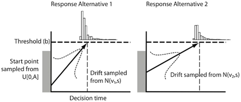
Figure 2. LBA model. The accumulator representing response alternative 1 is on average faster than the competing accumulator. The model therefore predicts that response alternative 1 will be selected on the majority of trials. See text for details.

In LBA and related response-time models, stimulus differences are often modeled by allowing drift rate to vary (e.g., Brown and Heathcote, 2008; Wagenmakers et al., 2008; Ho et al., 2009; Van Maanen et al., 2009; Van Maanen and Van Rijn, 2010). Therefore, in the first LBA model that we fit to the data (i.e., Model 1), we allowed the drift rate of the model to vary over the different angular distances, with all other parameters fixed. In addition to drift rate, Model 2 also allows the non-decision time to vary over the angles. Although there is no theoretical reason for this assumption, it is important to assess that in the data the non-decision time does not vary over angles, so that we can estimate a single value for γ. Models 3 and 4 are identical to Models 1 and 2 but in addition allow the drift rate variance to vary over angles (Churchland et al., 2011). Parameter values were optimized using quantile maximum likelihood estimation (Heathcote et al., 2002), using the 0.1, 0.3, 0.5, 0.7, and 0.9 quantiles of the RT distributions for correct and error responses.

Results and Discussion

We excluded trials in which the participants failed to respond in time (over 2000 ms, 3.3% of the trials) as well as trials in which the participants responded too fast (faster than 200 ms, 0.9%). Table 1 presents the mean accuracy per condition; Figure 3 presents MRT of the correct responses, for each participant separately. The results show that MRT decreases with the angular distance, whereas accuracy increases. This is consistent with the idea that smaller angular distances are more difficult and would therefore lead to more errors and slower correct responses. Participant 3 displays behavior that does not clearly follow this result, although the smallest angular distance yields slower responses than the widest angle. We could not find a reason why this participant displays behavior that does not follow our hypotheses. Therefore, there is no reason to exclude this participant from the analyses. However, it should be noted that the results do not hinge on this participant, and would stand even if we would exclude this participant.

TABLE 1

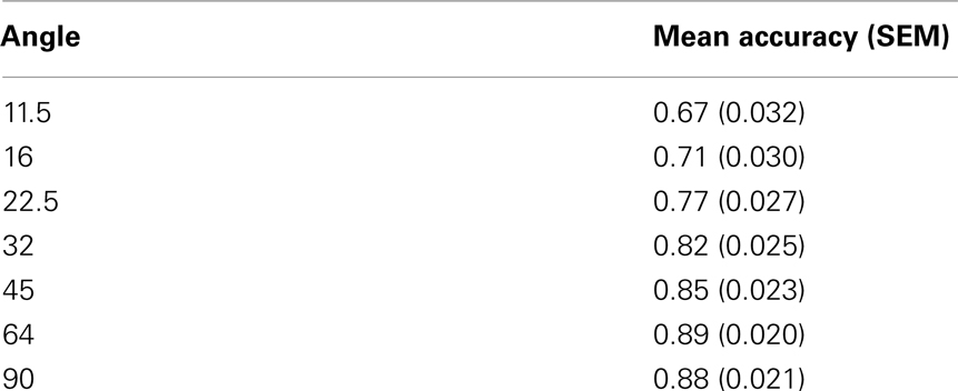
Table 1. Average accuracy scores per angular distance (and average within-subjects standard error of the mean, Loftus and Masson, 1994).

FIGURE 3

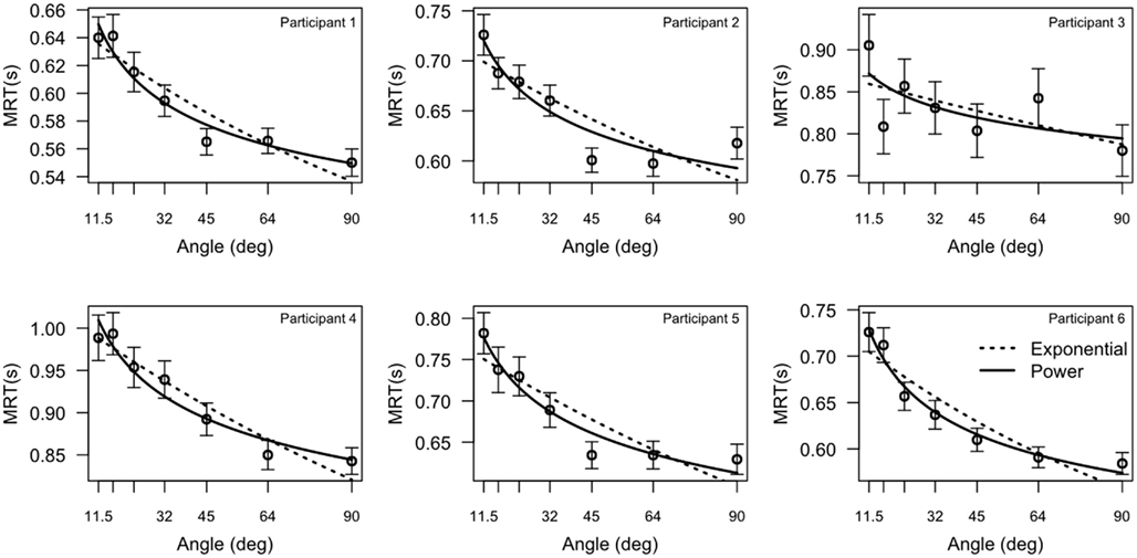
Figure 3. Mean response times (MRT) as a function of angular distance. Each plot represents the data from one participant. (Error bars represent within-subjects standard error of the mean, Loftus and Masson, 1994). The best fitting power function and the best fitting exponential function are overlaid.

Table 2 presents the goodness of fit of the power and exponential functions presented in Equations (2) and (3), as well as evidence ratios. The fact that the evidence ratios are between 0 and 1 indicates that there is slightly more evidence in favor of the exponential function than the power function.

TABLE 2

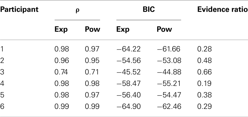
Table 2. Correlation coefficient (ρ), BIC values, and evidence ratios (Wagenmakers and Farrell, 2004) for the three-parameter power function and the exponential function for each participant.

It is misleading to accept these model results at face value, because the parameter estimates cannot be interpreted in psychological terms. A plausible interpretation of these functions should be that each response consists of a decision and additional processes such as stimulus encoding and response execution (cf. Sternberg, 1969; Luce, 1986). The additional processes are captured by the intercept γ, whereas the actual decision process is captured by the remaining time course. This interpretation entails that γ should be in a reasonable range of ∼200 to ∼500 ms. However, γ ranges here from 0 to 810 ms (Table 3). While a negative value for this parameter is impossible because it would suggest a negative duration³, a value of γ = 0 ms suggests that no time was required for processes unrelated to the decision. On the other hand, a value of γ = 810 ms is higher than some of the observed response times (and even higher than the MRT for large angles), which also makes it impossible to interpret γ as non-decision time. Thus, the under constraint of these non-linear models leads to implausible parameter estimates, and therefore the results lack psychological credibility. Because of the unexpected behavior of Participant 3, the best fitting parameters take different values than for the remaining participants.

TABLE 3

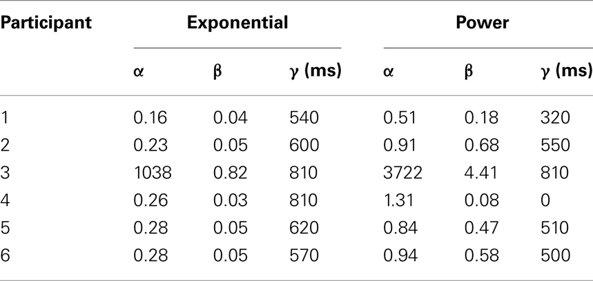
Table 3. Best fitting parameter values for the three-parameter power and exponential functions.

For these reasons, we take a more elaborate approach in fitting the power and exponential functions by first fitting an LBA model to the data and then estimating the parameters of the non-linear functions on the decision time. The LBA model that best balanced model fit with the number of free parameters was Model 1, the model in which only drift rate varied over angles. The average BIC value for Model 1 over participants was 7092, which was considerably less than any of the other models (7149, 8276, and 7307, respectively)⁴. Thus, the BIC results indicate that only drift rate variations were required to account for the data and no additional parameters were needed.

For Model 1, the best fitting parameter values are presented in Table 4⁵. As expected, the LBA model captures the increase in mean drift rate with increasing angular distance. The estimated non-decision time parameters (γ) seem to be in a reasonable range of 270–500 ms.

TABLE 4

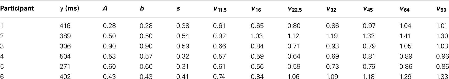
Table 4. Best fitting LBA model parameters for the data of Experiment 1.

A power function fits better

The LBA model allowed a more constrained estimation of the non-decision time parameter γ. We can now estimate power and exponential curves using this parameter estimate to assess whether the data follows a Piéron-like pattern. We fitted Equations (2) and (3) to the data of Experiment 1, allowing two free parameters (α and β), and one fixed parameter γ. Again, we fit both functions using standard simplex optimization routines (Nelder and Mead, 1965). The best fitting exponential and power curves are presented in Figure 3 (the best fitting parameters are presented in Table 6).

The results show that the power function was the best fitting model for all participants. Table 5 presents the goodness of fit for the exponential and power functions presented in Equations (3) and (2). The power function is consistently the better model, as indicated by the lower BIC values and higher correlations. Although the data of Participants 3 and 4 do not clearly distinguish between the models, the power function clearly is the better model for the remaining participants. In terms of the evidence ratio, the power function is 15 to 415 times more likely than the exponential function for these participants. This suggests that an increase in angular distance yields a power law decrease in MRT, and not an exponential law. The model comparison of the psychologically constrained models thus shows that behavior in 2AFC tasks is Piéron-like when the discriminability of choice alternatives is manipulated.

TABLE 5

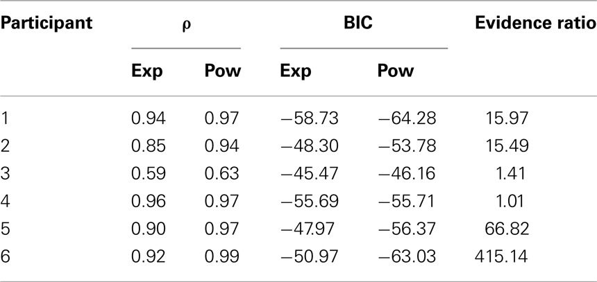
Table 5. Correlation coefficient (ρ) and BIC values for the two-parameter power function and the exponential function for each participant.

TABLE 6

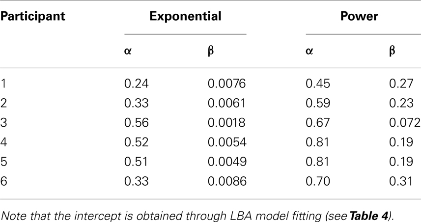
Table 6. Best fitting parameter values for the two-parameter power and exponential functions.

Bayesian Ideal Observer

In detection tasks, Piéron’s Law relates MRT to stimulus intensity by means of a power function (Equation 1). Experiment 1 showed that MRT and choice difficulty in a 2AFC task are also related by means of a power function. This result suggests that Piéron’s Law may generalize to choice behavior in which the discriminability of the correct alternative relative to the incorrect alternative is manipulated, instead of the intensity of the stimulus. To understand better why participants in Experiment 1 behave in accordance to Piéron’s Law, we developed a Bayesian ideal observer model. This model assumes that participants make the optimal choice, given the uncertainty of the task (for example, a noisy stimulus).

Methods

The RDM stimulus consists of a set of dots each moving in a particular direction. A proportion of dots move in the same direction whereas the remaining dots move in random directions. In order to make a correct decision, the observer needs to decide whether a certain amount of evidence for a particular response alternative outweighs the evidence for other response alternatives. If the observer performs this task on average in the minimum time required for a particular error rate, the observer is said to be optimal (Bogacz et al., 2006; Brown et al., 2009). Optimal behavior is achieved if the observer computes for each response alternative the posterior probability that it is the target based on the evidence observed so far (Baum and Veeravalli, 1994):

with H_i the hypothesis that motion direction i generated the RDM stimulus and x₁, …, x_t ∈ D the observed motion directions over time. Here we assume that the prior probabilities for each alternative are equal and hence can be ignored:

On the basis of new incoming evidence, the model continually updates the posterior probability of each response alternative, until the probability of one of the alternatives crosses a preset response criterion θ:

The time needed to reach that particular criterion θ determines the decision time (DT). Because in the current context we only discuss two-choice decisions, this equation reduces to a sequential probability ratio test (SPRT, Wald, 1947)

in which alternative 1 is chosen if θ* ≥ θ/(1 − θ) and alternative 2 is chosen if θ* ≤ (1 − θ)/θ (Baum and Veeravalli, 1994).

Results and Discussion

Piéron’s law in the ideal observer model for 2AFC tasks

We assume here that the evidence for the correct response alternative is represented by a Gaussian distribution with a mean μ_i representing the direction of motion. The variance of the distribution σ² may represent individual differences in perceptual ability, but will remain constant in our simulations. Thus, at each time step the model samples from the Gaussian distribution:

until the decision threshold has been reached⁶.

Without loss of generality we assume that the correct response is always alternative 1. The evidence for alternative 1 at any time step is computed from the Gaussian distribution function (Equation 5). Substituting Equation (5) in Equation (4) and taking the log shows that an evidence sample S_t for any alternative is proportional to the distance between the alternatives:

Following this computation of the evidence at each time step the ideal observer model predicts that decision times decrease as a power curve with the angular distance between the alternatives, as shown by Stafford and Gurney, 2004): Suppose that at each time step, the posterior probability of either alternative is increased with the average evidence sample E{S_t}. Then a decision is made as soon as with a decision time of approximately DT. Therefore DT·E{S_t} ≈ log θ*, which means that the mean decision time (MDT) is

with C = log θ*. Because S_t ∝ (μ₁ − μ₂)², Equation (7) entails Piéron’s Law (Equation 1) with the intercept γ = 0.The value of the scaling parameters α and β depends on the threshold and the variance in the assumed Gaussian distributions.

To corroborate this result, we explored the model’s behavior as a function of angular distance by running a 2AFC simulation. That is, the model had two response options and we manipulated the angular distance from 11.5° to 90°. In addition, we modeled a range of response criteria (from 0.6 to 0.9). The variance of the sampling distribution was kept constant at σ² = 4. The result of these simulations are presented in Figure 4. Each data point in Figure 4 was estimated using 10,000 Monte Carlo samples. The model’s behavior exhibits Piéron’s Law: when transformed to a log-log-scale the relation between angular distance and MDT is approximately linear. This pattern is observed independent of the response criterion (θ*) that is being adopted.

FIGURE 4

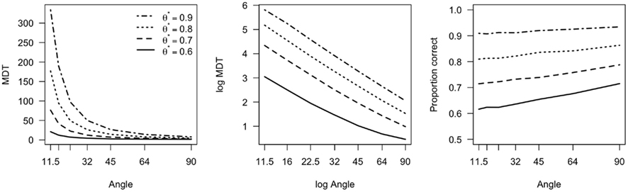
Figure 4. Ideal observer model behavior as a function of the angular distance between alternatives, for four different response criterion values. Left: Mean decision time (MDT) vs angular distance. Middle: log MDT vs log Angle. Right: Proportion correct vs Angle. θ*: response criterion value.

These simulations are in line with the results from Experiment 1, and together the model and experiment support the view that Piéron’s Law is a consequence of optimal behavior, at least in perceptual 2AFC tasks. To extend these results to the traditional field of application of stimulus detection, we demonstrate how the ideal observer model predicts Piéron’s Law in stimulus detection experiments.

Piéron’s law in the ideal observer model for stimulus detection

In stimulus detection experiments, the intensity of a stimulus is manipulated and participants are required to indicate the presence or absence of the stimulus. An ideal observer (ideal stimulus detector) weighs the likelihood of the presence of the stimulus (i.e., P(D|H₁) in Equation 4) against the likelihood of the absence of the stimulus (i.e., P(D|H₂)). Because any evidence supporting the presence (or absence) of the stimulus contributes equal evidence against the absence (or presence) of the stimulus, Equation (4) can be written as

Piéron’s Law emerges from an ideal observer model for stimulus detection if the likelihood of the presence (or absence) of the stimulus at each time step scales linearly with the stimulus intensity. In that case, MDT will decrease with stimulus intensity according to a power function (Equation 7) which will result in Piéron’s Law. Figure 5 presents the results of a simulation of this process. On each time step a value is drawn from a Gaussian distribution with stimulus intensity as the mean and σ = 0.005. The stimulus intensities ranged from 0.01 to 0.05. Equation (8) was computed until the posterior probability exceeded threshold (θ*), and the number of time steps required was recorded. Each data point in Figure 5 was estimated using 10,000 Monte Carlo samples. Again, the linearity in log-log space illustrates that the non-linear relation in the MRT data follows a power curve.

FIGURE 5

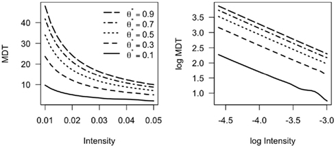
Figure 5. Ideal observer model behavior as a function of stimulus intensity, for five different response criterion values. Left: Mean decision time (MDT) vs stimulus intensity. Right: log MDT vs log Intensity. θ*: response criterion value.

General Discussion and Conclusion

Piéron’s Law has previously only been studied in experiments in which stimulus intensity was manipulated. Here, we hypothesized that Piéron’s Law may be a special case of a more general relationship between choice difficulty and mean response time. To support this conjecture, we performed an experiment in which the difficulty of choice in a random-dot motion paradigm was manipulated by adjusting the angular distance between two response alternatives. We found a power law relation between angular distance (discriminability) and mean response time, supporting our hypothesis of a general mechanism behind Piéron’s Law. A Bayesian ideal observer model showed that participants performing a 2AFC task may respond in a Piéron-like manner because it is the optimal way of minimizing overall response times (for a fixed error rate). The ideal observer model can also be extended to stimulus detection behavior, showing that Piéron’s Law reflects optimal detection behavior under varying stimulus intensities.

One particular aspect of our study deserves some additional consideration. We conclude that the decline of MRT with choice difficulty in Experiment 1 can be best described by a power function. An important step toward this conclusion was to determine which part of the observed response time we wanted to explain. As we have argued, directly fitting the models to the observed data does not provide enough constraint to make an appropriate model selection inference. Therefore, we first determined the decision time by subtracting an estimate for the non-decision time from the RTs. The non-decision time was estimated using the LBA model of choice-response time (Brown and Heathcote, 2008).

The validity of this approach rests on the extent to which it is reasonable to exclude non-decision time and focus on decision time. Because the exponential and power functions also implicitly focus on decision time, we believe that in this study, our approach is plausible. After subtracting non-decision time the evidence in favor of the power function was overwhelming, which was not the case for the models that were directly fitted to MRT. In some instances, the traditional approach may lead to an accurate estimate of the non-decision time parameter. In those cases, a more elaborate two-step fitting approach may not appear to be necessary. However, even in such cases we recommend the two-step fitting approach.

It should be noted that although we used a specific processing model to obtain appropriate non-decision time estimates (the LBA model), the same results could have been obtained with any other model that takes the variance in the RT distribution into account (e.g., Donkin et al., 2011). Where the LBA model is a full process model that attempts to describe many aspects of decision-making, we could have also used simpler process models (e.g., the EZ diffusion model, Wagenmakers et al., 2007), or even any descriptive model of the RT distribution (Matzke and Wagenmakers, 2009).

In summary, we have shown that MRT in a 2AFC task decreases with stimulus discriminability according to a power function. In addition, we provided a Bayesian ideal observer analysis of both 2AFC tasks and stimulus detection tasks. This analysis showed that optimal behavior in these tasks follows a power function when stimulus discriminability is manipulated. These results support the view that Piéron’s Law originates from optimal information processing.

Author Note

Leendert van Maanen, Raoul Grasman, Birte Forstmann, and Eric-Jan Wagenmakers, Department of Psychology, University of Amsterdam. Correspondence concerning this article should be addressed to Leendert van Maanen, Cognitive Science Center Amsterdam, University of Amsterdam, Plantage Muidergracht 24, 1018 TV Amsterdam, the Netherlands, e-mail: l.vanmaanen@uva.nl. We thank Helen Steingröver for data collection. This research was supported by VENI and VIDI grants from the Netherlands Organization for Scientific Research.

Conflict of Interest Statement

The authors declare that the research was conducted in the absence of any commercial or financial relationships that could be construed as a potential conflict of interest.

Footnotes

1. ^We use decision time to refer to the time required to make a choice in 2AFC tasks, and detection time to refer to the time required to detect a stimulus in a stimulus detection task.
2. ^The library can be downloaded from http://www.shadlen.org/Code/VCRDM.
3. ^We constrained the simplex routine to only allow positive values. Without this constraint, the best fitting models included values of γ < 0 ms.
4. ^These BIC values are higher than the BIC values obtained with the power and exponential functions because here we fit the quantiles instead of MRT.
5. ^The model fit itself is presented in the Appendix.
6. ^Because of the circular arrangement of response alternatives in the RDM task a slightly more accurate sampling distribution would be the von Mises distribution, which can be thought of as a Gaussian distribution wrapped around a circle. Because this distribution leads to similar results we chose to use the more generally applicable Gaussian.

References

Ball, K., and Sekuler, R. (1982). A specific and enduring improvement in visual motion discrimination. Science 218, 697–698.

Pubmed Abstract | Pubmed Full Text | CrossRef Full Text

Banks, W. (1973). Reaction time as a measure of summation of warmth. Percept. Psychophys. 13, 321–327.

CrossRef Full Text

Baum, C., and Veeravalli, V. (1994). A sequential procedure for multihypothesis testing. IEEE Trans. Inf. Theory 40, 1994–2007.

CrossRef Full Text

Bogacz, R., Brown, E., Moehlis, J., Holmes, P., and Cohen, J. D. (2006). The physics of optimal decision making: a formal analysis of models of performance in two-alternative forced-choice tasks. Psychol. Rev. 113, 700–765.

Pubmed Abstract | Pubmed Full Text | CrossRef Full Text

Bonnet, C., Zamora, M. C., Buratti, F., and Guirao, M. (1999). Group and individual gustatory reaction times and Piéron’s law. Physiol. Behav. 66, 549–558.

Pubmed Abstract | Pubmed Full Text | CrossRef Full Text

Brainard, D. H. (1997). The psychophysics toolbox. Spat. Vis. 10, 433–436.

Pubmed Abstract | Pubmed Full Text | CrossRef Full Text

Britten, K. H., Shadlen, M. N., Newsome, W. T., and Movshon, J. A. (1992). The analysis of visual motion: a comparison of neuronal and psychophysical performance. J. Neurosci. 12, 4745–4765.

Pubmed Abstract | Pubmed Full Text

Brown, S., and Heathcote, A. (2008). The simplest complete model of choice response time: linear ballistic accumulation. Cogn. Psychol. 57, 153–178.

Pubmed Abstract | Pubmed Full Text | CrossRef Full Text

Brown, S., Steyvers, M., and Wagenmakers, E.-J. (2009). Observing evidence accumulation during multi-alternative decisions. J. Math. Psychol. 53, 453–462.

CrossRef Full Text

Chocholle, R. (1940). Variation des temps de réaction auditifs en fonction de l’intensité à diverses fréquences. Année Psychol. 41, 65–124.

CrossRef Full Text

Churchland, A. K., Kiani, R., Chaudhuri, R., Wang, X.-J., Pouget, A., and Shadlen, M. N. (2011). Variance as a signature of neural computations during decision making. Neuron 69, 818–831.

Pubmed Abstract | Pubmed Full Text | CrossRef Full Text

Churchland, A. K., Kiani, R., and Shadlen, M. N. (2008). Decision-making with multiple alternatives. Nat. Neurosci. 11, 693–702.

Pubmed Abstract | Pubmed Full Text | CrossRef Full Text

Donkin, C., Brown, S., Heathcote, A., and Wagenmakers, E. (2011). Diffusion versus linear ballistic accumulation: different models but the same conclusions about psychological processes? Psychon. Bull. Rev. 18, 61–69.

Pubmed Abstract | Pubmed Full Text | CrossRef Full Text

Forstmann, B. U., Anwander, A., Schäfer, A., Neumann, J., Brown, S., Wagenmakers, E.-J., Bogacz, R., and Turner, R. (2010a). Cortico-striatal connections predict control over speed and accuracy in perceptual decision making. Proc. Natl. Acad. Sci. U.S.A. 107, 15916–15920.

CrossRef Full Text

Forstmann, B. U., Brown, S. D., Dutilh, G., Neumann, J., and Wagenmakers, E. J. (2010b). The neural substrate of prior information in perceptual decision making: a model-based analysis. Front. Hum. Neurosci. 4:40. doi:10.3389/fnhum.2010.00040

CrossRef Full Text

Forstmann, B. U., Dutilh, G., Brown, S., Neumann, J., von Cramon, D. Y., Ridderinkhof, K. R., and Wagenmakers, E. J. (2008). Striatum and pre-SMA facilitate decision-making under time pressure. Proc. Natl. Acad. Sci. U.S.A. 105, 17538–17542.

Pubmed Abstract | Pubmed Full Text | CrossRef Full Text

Heathcote, A., Brown, S., and Mewhort, D. J. K. (2002). Quantile maximum likelihood estimation of response time distributions. Psychon. Bull. Rev. 9, 394–401.

Pubmed Abstract | Pubmed Full Text | CrossRef Full Text

Ho, T. C., Brown, S., and Serences, J. T. (2009). Domain general mechanisms of perceptual decision making in human cortex. J. Neurosci. 29, 8675–8687.

Pubmed Abstract | Pubmed Full Text | CrossRef Full Text

Jaskowski, P., and Sobieralska, K. (2004). Effect of stimulus intensity on manual and saccadic reaction time. Percept. Psychophys. 66, 535–544.

Pubmed Abstract | Pubmed Full Text | CrossRef Full Text

Loftus, G. R., and Masson, M. (1994). Using confidence intervals in within-subject designs. Psychon. Bull. Rev. 1, 476–490.

CrossRef Full Text

Luce, R. D. (1986). Response Times. New York: Oxford University Press.

Matzke, D., and Wagenmakers, E.-J. (2009). Psychological interpretation of the ex-Gaussian and shifted Wald parameters: a diffusion model analysis. Psychon. Bull. Rev. 16, 798–817.

Pubmed Abstract | Pubmed Full Text | CrossRef Full Text

Mulder, M., Bos, D., Weusten, J. M., van Belle, J., Dijk, S. C., Simen, P., van Engeland, H., and Durston, S. (2010). Basic impairments in regulating the speed-accuracy tradeoff predict symptoms of ADHD. Biol. Psychiatry 68, 1114–1119.

Pubmed Abstract | Pubmed Full Text | CrossRef Full Text

Nelder, J., and Mead, R. (1965). A simplex method for function minimization. Comput. J. 7, 308–313.

Niwa, M., and Ditterich, J. (2008). Perceptual decisions between multiple directions of visual motion. J. Neurosci. 28, 4435–4445.

Pubmed Abstract | Pubmed Full Text | CrossRef Full Text

Overbosch, P., de Wijk, R., de Jonge, T. J., and Köster, E. P. (1989). Temporal integration and reaction times in human smell. Physiol. Behav. 45, 615–626.

Pubmed Abstract | Pubmed Full Text | CrossRef Full Text

Palmer, J., Huk, A. C., and Shadlen, M. N. (2005). The effect of stimulus strength on the speed and accuracy of a perceptual decision. J. Vis. 5, 376–404.

Pubmed Abstract | Pubmed Full Text | CrossRef Full Text

Piéron, H. (1914). Recherches sur les lois de variation des temps de latence sensorielle en fonction des intensités excitatrices. Année Psychol. 22, 17–96.

Pins, D., and Bonnet, C. (1996). On the relation between stimulus intensity and processing time: Piéron’s law and choice reaction time. Percept. Psychophys. 58, 390–400.

Pubmed Abstract | Pubmed Full Text | CrossRef Full Text

Raftery, A. (1996). “Hypothesis testing and model selection,” in Markov Chain Monte Carlo in Practice, eds W. Gilks, S. Richardson, and D. Spiegelhalter (Boca Raton, FL: Chapman & Hall/CRC), 163–187.

Salzman, C. D., and Newsome, W. T. (1994). Neural mechanisms for forming a perceptual decision. Science 264, 231–237.

Pubmed Abstract | Pubmed Full Text | CrossRef Full Text

Schwarz, G. (1978). Estimating the dimension of a model. Ann. Stat. 6, 461–464.

CrossRef Full Text

Shadlen, M. N., and Newsome, W. T. (2001). Neural basis of a perceptual decision in the parietal cortex (area LIP) of the rhesus monkey. J. Neurophysiol. 86, 1916–1936.

Pubmed Abstract | Pubmed Full Text

Stafford, T., and Gurney, K. N. (2004). The role of response mechanisms in determining reaction time performance: Piéron’s law revisited. Psychon. Bull. Rev. 11, 975–987.

Pubmed Abstract | Pubmed Full Text | CrossRef Full Text

Stafford, T., Ingram, L., and Gurney, K. N. (2011). Piéron’s law holds during Stroop conflict: insights into the architecture of decision making. Cogn. Sci. 35, 1553–1566.

Pubmed Abstract | Pubmed Full Text | CrossRef Full Text

Sternberg, S. (1969). The discovery of processing stages: extensions of Donders’ method. Acta Psychol. (Amst.) 30, 276–315.

CrossRef Full Text

Van Maanen, L., Brown, S. D., Eichele, T., Wagenmakers, E. J., Ho, T. C., Serences, J. T., and Forstmann, B. U. (2011). Neural correlates of trial-to-trial fluctuations in response caution. J. Neurosci. 31, 17488–17495.

Pubmed Abstract | Pubmed Full Text | CrossRef Full Text

Van Maanen, L., and Van Rijn, H. (2010). The locus of the Gratton effect in picture-word interference. Top. Cogn. Sci. 2, 168–180.

CrossRef Full Text

Van Maanen, L., Van Rijn, H., and Borst, J. P. (2009). Stroop and picture-word interference are two sides of the same coin. Psychon. Bull. Rev. 16, 987–999.

Pubmed Abstract | Pubmed Full Text | CrossRef Full Text

Wagenmakers, E.-J., and Farrell, S. (2004). AIC model selection using Akaike weights. Psychon. Bull. Rev. 11, 192–196.

Pubmed Abstract | Pubmed Full Text | CrossRef Full Text

Wagenmakers, E.-J., Ratcliff, R., Gomez, P., and McKoon, G. (2008). A diffusion model account of criterion shifts in the lexical decision task. J. Mem. Lang. 58, 140–159.

Pubmed Abstract | Pubmed Full Text | CrossRef Full Text

Wagenmakers, E.-J., van der Maas, H. L. J., and Grasman, R. P. P. P. (2007). An EZ-diffusion model for response time and accuracy. Psychon. Bull. Rev. 14, 3–22.

Pubmed Abstract | Pubmed Full Text | CrossRef Full Text

Wald, A. (1947). Sequential Analysis. New York: Wiley.

Appendix

Figures A1–A6 present the fit of the Linear Ballistic Accumulator (LBA) model to the data of Experiment 1. Each figure represents the data (black circles) and model fit (red lines) for one participant. The top line represents the cumulative RT distribution of correct responses, the bottom line represents the cumulative RT distribution of incorrect responses. Both lines are weighted to the probability of an incorrect response. Each graph represents the different angular distances (d) used in Experiment 1.

FIGURE A1

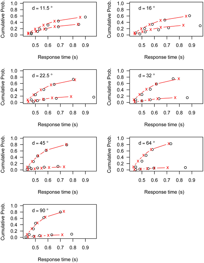
Figure A1. LBA model fit for Participant 1.

FIGURE A2

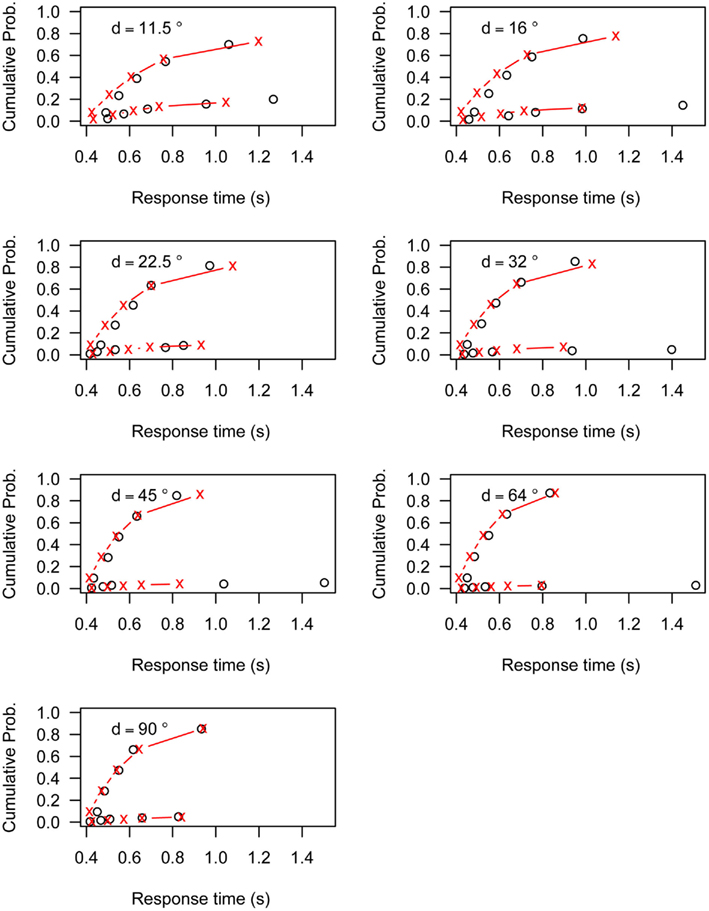
Figure A2. LBA model fit for Participant 2.

FIGURE A3

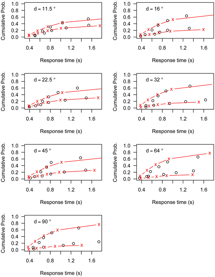
Figure A3. LBA model fit for Participant 3.

FIGURE A4

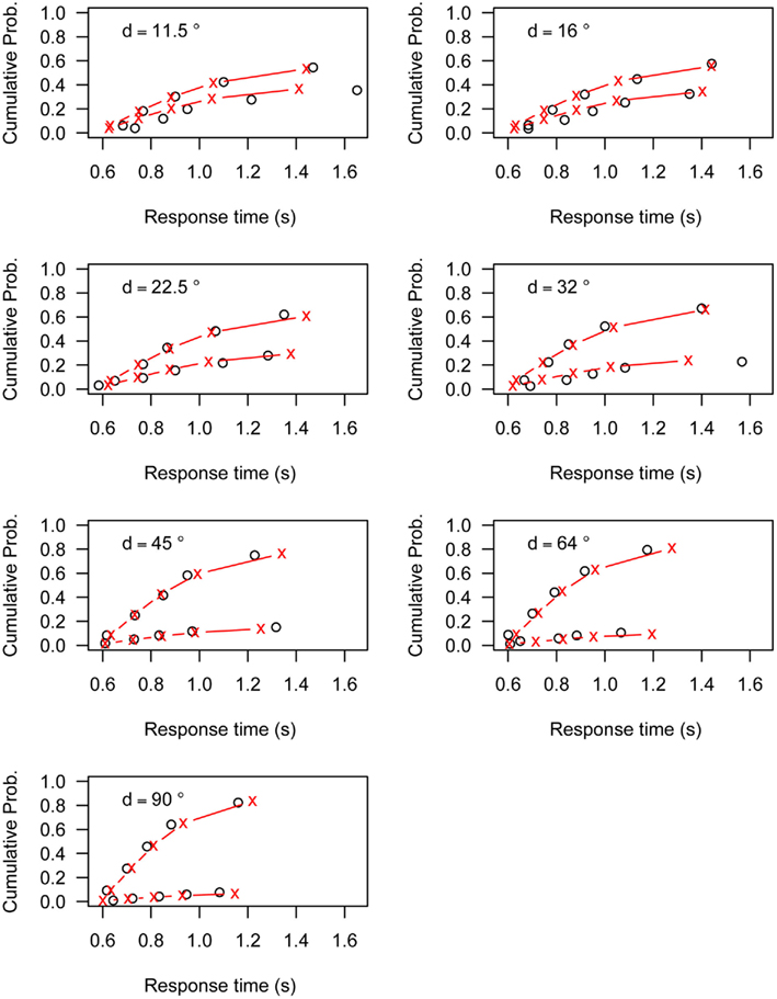
Figure A4. LBA model fit for Participant 4.

FIGURE A5

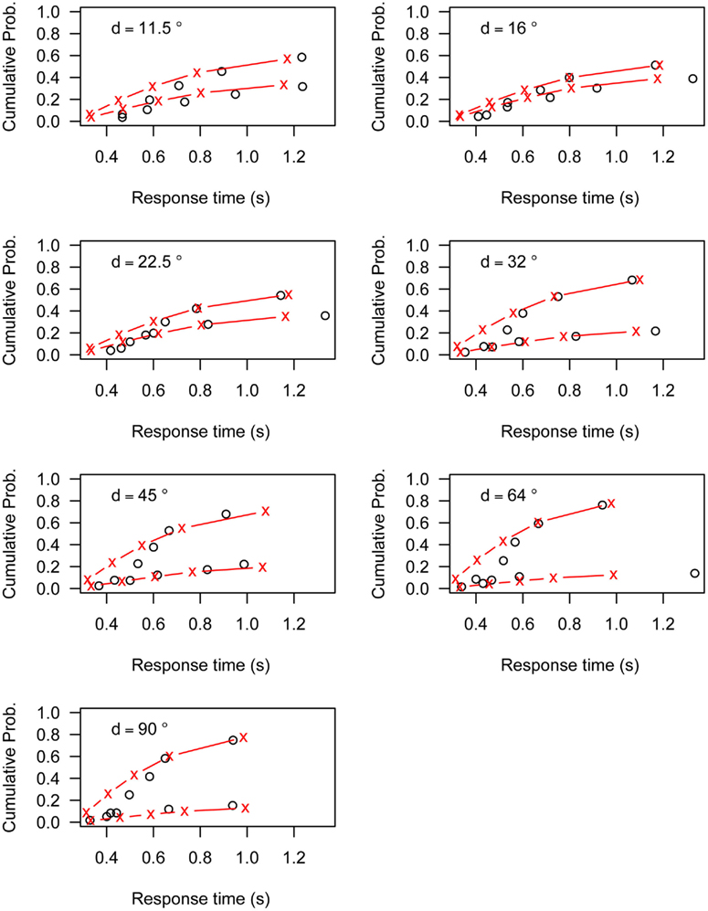
Figure A5. LBA model fit for Participant 5.

FIGURE A6

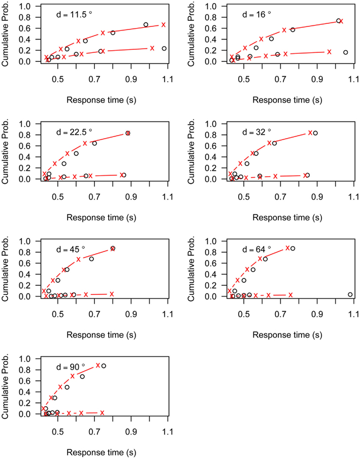
Figure A6. LBA model fit for Participant 6.