Using Lidar Data to Assess the Relationship Between Beach Geomorphology and Kemp’s Ridley (Lepidochelys kempii) Nest Site Selection Along Padre Island, TX, United States

Introduction

The range of the Kemp’s ridley sea turtle encompasses the Gulf of Mexico and extends into the northwestern Atlantic Ocean (Putman et al., 2013). Most nesting occurs on beaches along the west-central Gulf of Mexico, with the greatest nesting numbers near Rancho Nuevo, Tamaulipas, Mexico (Shaver and Rubio, 2008; Caillouet et al., 2015; Shaver and Caillouet, 2015). The Mexican government began protecting the nests in 1966 because the population was rapidly declining (Caillouet et al., 2015; Shaver and Caillouet, 2015). By 1977, extinction of the species was imminent, so a bi-national, multi-agency imprinting and head-start project was implemented in order to increase Kemp’s ridley nesting at Padre Island National Seashore (PAIS), known as the PAIS Restoration Program (Shaver and Rubio, 2008; Shaver and Caillouet, 2015). The overall goal of this project was to create a secondary nesting colony in a location that was both protected and within the native range of the species (Shaver and Rubio, 2008). Due to these and other efforts, both Rancho Nuevo and Padre Island National Seashore serve as main nesting sites for the Kemp’s ridley sea turtle today, in Mexico and the United States, respectively (Caillouet et al., 2015). Nesting also occurs in Veracruz, Mexico and occasionally in Florida, Alabama, and the Atlantic coast in the United States (National Marine Fisheries Service and U. S. Fish and Wildlife Service, 2015).

A female sea turtle responds to various signals, both biotic and abiotic, to select the most successful site for her eggs, making nest site selection non-random (Weishampel et al., 2006; Zavaleta-Lizárraga and Morales-Mávil, 2013). According to Wood and Bjorndal (2000), sea turtle nest site selection can be divided into three stages: beach selection, emergence of the female, and nest placement. Beach selection and emergence probably depend on offshore cues and beach characteristics, such as slope and dune profile (Wood and Bjorndal, 2000). A number of selective forces drive nest placement both seaward toward the shoreline and landward away from it; nests close to the sea have a higher probability of inundation and egg loss due to erosion while nests further from the sea are more likely to result in predation and hatchling disorientation (Wood and Bjorndal, 2000; Santos et al., 2006).

The biophysical features of beaches that affect nest site selection have long been thoroughly studied, but morphological characteristics influencing nest site selection have not been researched to the same extent (Horrocks and Scott, 1991; Yamamoto et al., 2012). There has been little to no research regarding the connection between beach geomorphology and Kemp’s ridley nesting site selection, but studies regarding other species of sea turtles suggest that beach characteristics may be important factors in determining sea turtle nesting site preferences (Santos et al., 2006; Yamamoto et al., 2012).

While it is well-known that females prefer to nest on beaches with fine grain sands because it is more difficult to dig egg chambers in coarse, dry sand, Mortimer (1982) predicted that slope and offshore configuration are potentially more important than sand grain properties in nesting preferences, but their relative importance was not quantified (Mortimer, 1982, 1990). One study found that segments of beaches with higher beach face slopes and narrower widths had higher nest densities of loggerhead turtles than beaches with lower slopes and wider widths (Provancha and Ehrhart, 1987). Research regarding hawksbill turtles found that nest elevation above sea level was positively related to hatching success. Furthermore, this study found that hawksbills nested further from the high tide line on beaches with less steep slopes, suggesting that they prefer to nest at a certain mean elevation above sea level (Horrocks and Scott, 1991). Similarly, Wood and Bjorndal (2000) found that out of the factors slope, temperature, moisture, and salinity, slope had the largest impact on nest site selection of loggerheads, likely because it is correlated with nest elevation. A study in Mexico discovered that green sea turtles prefer beaches with steeper slopes, specifically a steeper berm slope, while hawksbill turtles nest site selection extended to a wider range of beach morphology characteristics (Cuevas et al., 2010). A similar study regarding nest site selection by the green sea turtle in Mexico found that the most utilized nest sites were characterized by beaches at least 1,300 m long with gentle to medium slopes (Zavaleta-Lizárraga and Morales-Mávil, 2013).

Most recently, Dunkin et al. (2016) developed a model that accurately predicted loggerhead nesting habitat suitability in Florida using elevation, beach slope, beach width, and dune peak as predictors. Consistent with the findings of several of the aforementioned studies, they found that elevation was the most influential factor for nesting preferences (Dunkin et al., 2016). Similarly, Yamamoto et al. (2012) successfully modeled nest density for three different sea turtle species using a limited number of geomorphology variables. This study found that each sea turtle species exhibited a tolerance for beaches with a wide range of measured geomorphology variables but would not nest on beaches outside of this tolerance (Yamamoto et al., 2012).

The specific preference of nesting beach characteristics varies between species, possibly due to the difference in size, weight, and behavior between each species. This makes the specific preference of nesting beach characteristics for the Kemp’s ridley difficult to quantify. Considering the importance that slope and elevation have in regards to nest site selection of various species of sea turtles, it is possible that they are important aspects of Kemp’s ridley nesting preference. Additionally, other geomorphology features, such as dune height, rugosity, aspect, beach width, distance from shoreline, and offshore configuration, might also be important aspects of nesting preference for the Kemp’s ridley. Marquez-M (1994) notes that on beaches in Rancho Nuevo, Mexico, the Kemp’s ridley usually nests beyond the high tide line in front of the first dune, on the windward slope of the dune or on top of the dune. This report describes the distribution of nests at relative positions along a beach profile, but it fails to quantify the characteristics of each position, such as elevation or distance from shoreline, and to assess alongshore nesting preferences in relation to beach geomorphology characteristics, such as beach slope or width (Marquez-M, 1994).

The purpose of this study is to: (1) identify the terrestrial habitat variability of the Kemp’s ridley sea turtle on the beaches of North and South Padre Islands, Texas; and (2) quantify the influence of beach geomorphology characteristics on Kemp’s ridley nest site selection.

Materials and Methods

Study Area

The study area for this research is the beaches of the Padre Island National Seashore, located on North Padre Island, and South Padre Island, TX, United States (Figure 1). North and South Padre Islands are barrier islands that run parallel to the coastline, separated from the mainland by the shallow estuaries of the Upper and Lower Laguna Madre, respectively (Judd et al., 1977; Weise and White, 2007). Collectively, North and South Padre Islands extend 182 km from Corpus Christi to Brazos-Santiago Pass, varying from 450 m to 4.8 km in width (Judd et al., 1977). Port Mansfield Channel is a human-made and jettied channel that separates South Padre Island from North Padre Island (Judd et al., 1977). Because Kemp’s ridleys have been observed nesting from the water line to behind the foredune crest, the study area includes the area of beach extending from the wet/dry line to the landward dune boundary.

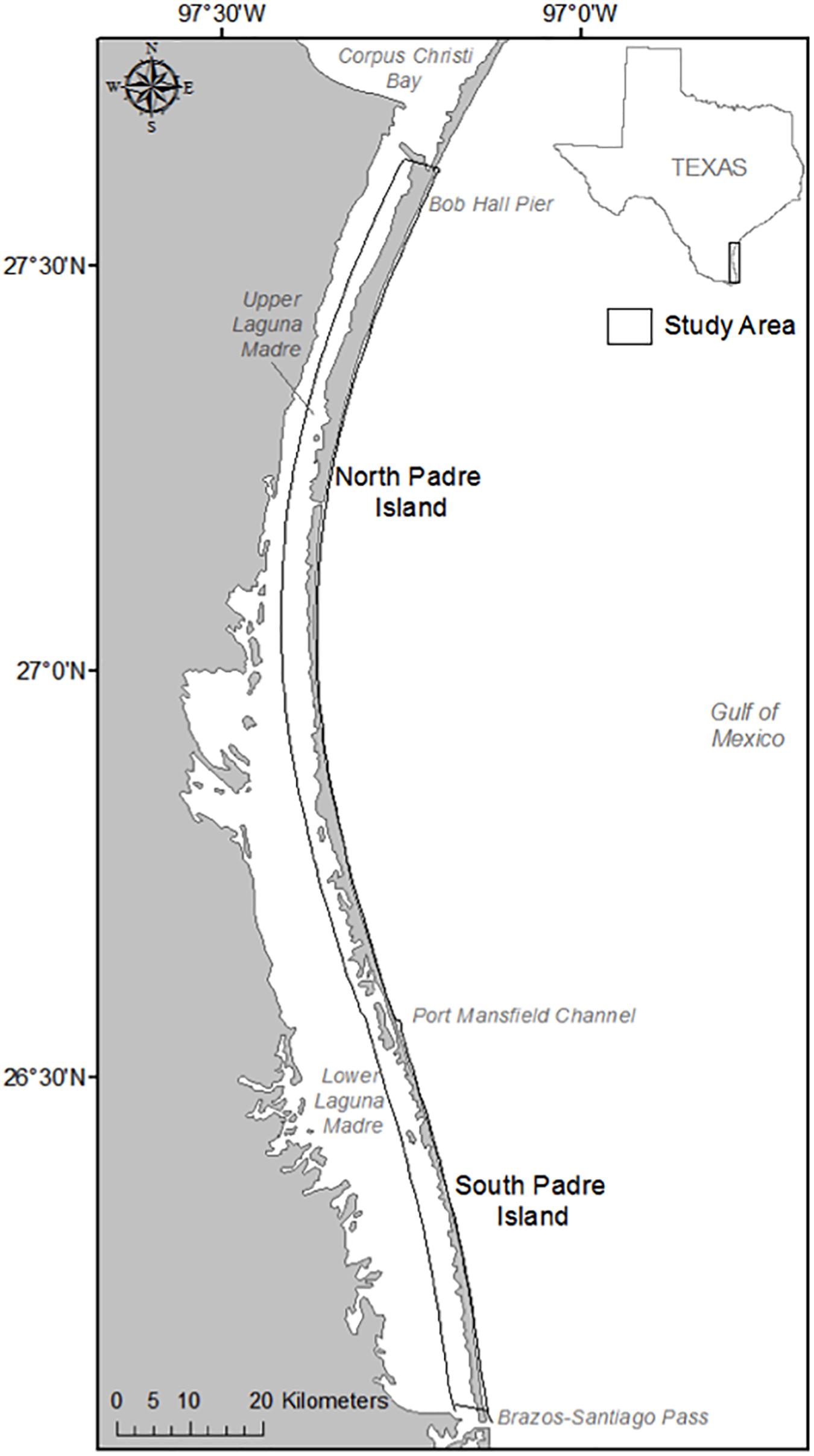
Figure 1. The study area of the research, the beaches of North and South Padre Islands, TX, United States.

Beaches in the northern and southern sections of the study area are broad and characterized by large foredunes and grasslands (Davis, 1977; Weise and White, 2007). Washover channels and a greater extent of development also characterize the southern section (Weise and White, 2007). The shape of the Texas Gulf shoreline causes longshore currents to converge near the central section of the study area, resulting in the accumulation of sediment and shell fragments (Davis, 1977). Thereby, the beaches in this region are steeper and the mean sediment size is larger in comparison to the other regions of the study area, resembling the geomorphology of the beaches of Rancho Nuevo, Mexico (Watson, 1971; Carranza-Edwards et al., 2004; Weise and White, 2007).

Dataset

The coordinates of observed Kemp’s ridley nests within the study area for the years 2009–2012 were obtained from Dr. Donna J. Shaver, the coordinator of the Sea Turtle Stranding and Salvage Network in Texas and Chief of Sea Turtle Science and Recovery at Padre Island National Seashore (Supplementary Table 1). The coordinates were imported into ArcGIS as XY data tables and were subsequently exported as shapefiles and projected to the coordinate system of UTM Zone 14 N. Of the total 573 nest coordinates, 8 points (1.39%) were determined to be outliers and were excluded from the study. These coordinates, comprised of three points from 2012, four points from 2011, and 1 point from 2010, were located outside of the study area, likely due to an instrumentation error when the nest coordinates were recorded.

Pseudo-absence points, or background data, establishes the characteristics of the study area while the presence data provides the attributes of the area in which a species is more likely to be present (Phillips et al., 2009). Barbet-Massin et al. (2012) found that model accuracy increased until an asymptote when the ratio of pseudo-absence to presence points reached 10:1 for generalized linear models and random forests, the statistical models used in this study. Therefore, psuedo-absence points were created randomly within the study area at a 10:1 ratio to the presence data.

In 2009, the US Army Corps of Engineers (USACE) Joint Airborne Lidar Bathymetry Technical Center of Expertise (JALBTCX) collected lidar data of the South Texas Gulf of Mexico shoreline for the West Texas Aerial Survey 2009 project. The survey was conducted between February and April, just before Kemp’s ridley nesting season. Additionally, the Bureau of Economic Geology (BEG), the Center for Space Research, and Texas A&M-Corpus Christi conducted three airborne lidar surveys of the Texas Gulf of Mexico shoreline every year from 2010 through 2012. The 2010 and 2011 surveys were conducted in April at the beginning of Kemp’s ridley nesting season while the 2012 survey was conducted in February, a few months prior to the start of nesting season (Paine et al., 2013). The las files for each dataset were procured from the NOAA Coastal Services Center’s Digital Coast website with NAD83 horizontal and NAVD88 vertical datums. Using NOAA/NOS’s VDatum, the USACE data was converted from Geoid12A to Geoid99, the same geoid as the 2010–2012 BEG lidar data. The BEG lidar data was characterized by UTM Zone 14 N projected coordinate system. Consequently, LAStools was used to project the 2009 LAS files into UTM Zone 14 N.

The last return points were used for this project in order to reduce the probability of land cover biasing topography (Starek Michael et al., 2012). The point density of each dataset was evaluated in order to determine the ideal resolution for the digital elevation models (DEMs) and outliers were located by identifying data points that exceed a height or slope difference relative to neighboring measurements within 30 m. Based on the point density of the datasets, a pixel size of 1 m was determined to be sufficient. Each LAS file was gridded using an inverse distance weighted (IDW) operation with a search radius of 2.5 m and a maximum of 3 points within each search radius. The subsequent rasters were combined to create consistent surfaces for each year.

Feature Extraction

Shoreline, potential line of vegetation, and landward dune boundaries were mapped to delineate the beach and the foredune complex within the study area for geomorphology characteristic extraction. Through the analysis of lidar data and beach profiles, Gibeaut et al. (2002) and Gibeaut and Caudle (2009) found that the wet/dry boundary typically occurs at 0.6 m above mean sea level on the Texas Gulf Coast. This elevation was mapped as the shoreline for each year. The potential vegetation line is the lowest elevation dune vegetation may thrive along the Texas Gulf shore and is 1.2 m above mean sea level. The wet/dry line is the seaward boundary of the beach and potential vegetation line is the landward boundary of the beach and seaward boundary of the foredune. The ArcGIS Contour List tool was used to map the contours, and the contours were smoothed using a 5 m tolerance with the Polynomial Approximation with Exponential Kernel (PAEK) method of the Smooth Line tool in ArcGIS. The landward dune boundaries for the 2010–2012 data were mapped by the Coastal and Marine Geospatial Lab at Harte Research Institute, as outlined in Paine et al. (2013). The same systematic qualitative criteria used to generate the landward dune boundaries for 2010–2012 was used to create a landward dune boundary for 2009.

Using the ET Geowizard Extension of ArcGIS, cross-shore profiles were created at each presence and pseudo-absence point, which were then delineated by beach, or the area between the shoreline and PVL, and dune system, or the area between the PVL and landward dune boundary. Points were created every 1 m along the profiles, and elevation values from the DEMs for each year were extracted to each. The points were converted back to line segments, resulting in 3D cross-shore profiles, from which various characteristics were derived. The resulting geomorphology characteristics include beach slope, beach width, dune peak height, dune slope uphill, and dune width (Table 1).

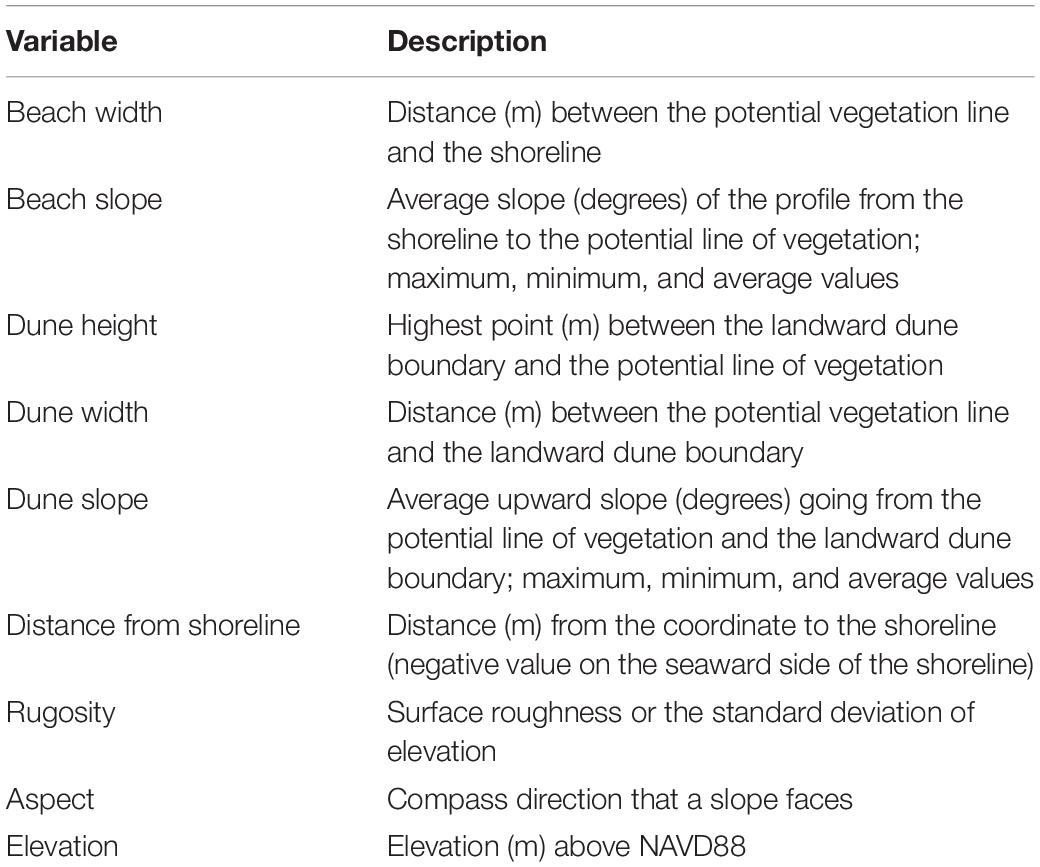
Table 1. Description of each geomorphology characteristic extracted to each presence and pseudo-absence point.

Using the ET Geowizard Extension of ArcGIS, the distance of each point from the shoreline was calculated by generating and measuring a line segment that extends from each point to the shoreline. Additionally, aspect, and rugosity rasters were created for each year from the DEMs. Values from the aspect, slope, and elevation ratsters were attributed to each coordinate for each year.

Analysis

To better understand the dynamics of the system, preliminary statistical analyses were conducted. The Optimized Hot Spot Analysis tool in ArcGIS, which identifies statistically significant spatial clusters of high values and low values, was used on each year of nest coordinates, as well as all years combined. This tool aggregates incident data, identifies an appropriate scale of analysis, and corrects for multiple testing and spatial dependence. The Getis_Ord Gi^∗ statistic is calculated for each feature in the dataset, and the resulting high and low z-scores are indicative of hot spots and cold spots, respectively. The resulting maps identified statistically significant hot spots and cold spots of nests and classified the general spatial trends in nesting.

Boxplots were created in R that compare the median and interquartile range of each geomorphology characteristic differentiated by nest presence and pseudo-absence. These boxplots served as tools that can be used to recognize if the Kemp’s ridleys are nesting within a subset of the available habitat. Additionally, a correlation matrix composed of pairwise scatterplots and associated Pearson correlation coefficients was calculated in R to assess the collinearity between the geomorphology characteristics and to preliminarily pinpoint any geomorphology characteristics with a relationship to nest presence. Collinearity between variables can skew generalized linear models, so this information was taken into consideration during model development and selection.

In addition, the data was analyzed using statistical regression models to both quantify the relationship between beach geomorphology characteristics and Kemp’s ridley nest site selection and assess the capacity of geomorphology characteristics in predicting nest presence. A generalized linear model was selected as a traditional modeling technique because it has the capacity of modeling response variables with non-normal distributions, such as discrete, binary data (Gilmour et al., 1985; Zuur et al., 2009). This modeling technique was expanded upon by the use of a machine-learning technique because recent studies have suggested that machine-learning methods may perform better than traditional algorithms, especially when the dataset includes a limited number of samples over an extensive range (Breiman, 2001; Elith et al., 2006; Mi et al., 2017).

Generalized Linear Models

Because the response variable is binary, binomial generalized linear models for all years of data combined were developed in R, with nest presence/absence as the dependent variable and the geomorphology characteristics as the explanatory variables. Models utilizing all explanatory variables were dredged in order to pinpoint the variables that comprise the relatively best model options. The best models options were then generated and evaluated using McFadden’s pseudo R-squared value, K-fold cross-validation prediction error, and a boxplot of the predictions differentiated by the observation value. McFadden’s pseudo R-squared value is defined as

where L_c denotes the likelihood value from the current fitted model and L_null denotes the corresponding value for the null model (McFadden, 1974). In K-fold cross-validation, the observations are split into K partitions, the model is trained on K-1 partitions, and the test error is predicted on the left out partition k (Zuur et al., 2009). This process is repeated for each partition and the result is the average test error of all partitions (Zuur et al., 2009).

Because the sampling type and ratio of the pseudo-absence data can greatly affect the model, these components were taken into consideration when developing the model (VanDerWal et al., 2009; Barbet-Massin et al., 2012). As mentioned in Section “Dataset,” pseudo-absence points were generated at a ratio of 10:1 to the presence points. However, using this ratio as an input into the model would likely cause the model to be biased to predict the pseudo-absence points. Therefore, models were developed using 10:1, 5:1, 2:1, and equal ratios of pseudo-absence points to presence points in order to gauge the effect of variations in ratio pseudo-absence points on model accuracy (VanDerWal et al., 2009; Barbet-Massin et al., 2012). The models generated using a 5:1, 2:1, and equal ratios of pseudo-absence to presence points were re-constructed 100 times, resampling the pseudo-absence points each iteration, in order to fully take into consideration the distribution of the pseudo-absence points. McFadden’s pseudo R-squared value, K-fold cross-validation prediction error, boxplots of the predictions differentiated by observed values, and the results of confusion matrices for each model were compared in order to evaluate model performance.

The analysis of spatial data is often complicated by spatial autocorrelation, a phenomenon that occurs when the values of variables sampled at nearby locations are not independent of each other (Dormann et al., 2007; Crase et al., 2014). In order to determine if there was spatial autocorrelation in the presence/absence data, a spline correlogram of the raw data was created in R (Zuur et al., 2009; Crase et al., 2014). A spline correlogram is a graphical representation of Moran’s I for different distance classes that is smoothed using a spline function. A spline correlogram of the Pearson residuals of the model was also created in R to determine if any spatial autocorrelation was explained by the explanatory variables (Zuur et al., 2009).

Random Forest

A random forest model was determined to be a suitable machine learning methodology option due to the size of the dataset and the binary nature of the predictant (Breiman, 2001; Svetnik et al., 2003; Elith et al., 2006; Mi et al., 2017). Specifically, a random forest was preferred over other machine-learning techniques, such as a neural network, because they are less computationally expensive, do no require an extensive amount of data, are less prone to overfitting and provide information on the importance of each predictor (Breiman, 2001).

Random forests are machine learning classification and regression tools composed of a combination of trees created by using bootstrap samples of training data and random feature selection in tree induction (Breiman, 2001; Svetnik et al., 2003). A random forest model was applied to the all of the years of data combined, with the predictant as the presence or pseudo-absence of a nest site and the predictors as the geomorphology characteristics. The relative importance of each predictor in the model was quantified, providing even more insight into the relationships within the system.

As previously mentioned in regards to the development of the generalized linear models, the sampling type and ratio of the pseudo-absence data can greatly affect the model, so these components were taken into consideration during the development the random forest model as well (VanDerWal et al., 2009; Barbet-Massin et al., 2012). A subset of the pseudo-absence points of equal ratio to the presence points was constructed and then the data was further split into 75% for testing and 25% for training. The random forest model was built and then a loop was established to perform 100 iterations of each step. This effectively bootstraps the pseudo-absence data so the entire distribution is assessed. In order to assess the accuracy of each model, a confusion matrix was generated as an output for both the test subset of each model. Accuracy, sensitivity, and specificity were used to assess and compare the performance of each model iteration. Variable important plots were constructed in order to determine the role of each explanatory variable.

Results

The use of the Optimized Hot Spot Analysis tool on the nest coordinates of each year and all years combined resulted in the presence of a hot spot near the central section of Padre Island, Texas each year (Figure 2). In particular, the analysis of all years combined exposed a notable hot spot along the central section of Padre Island and a cold spot along the northern half of South Padre Island.

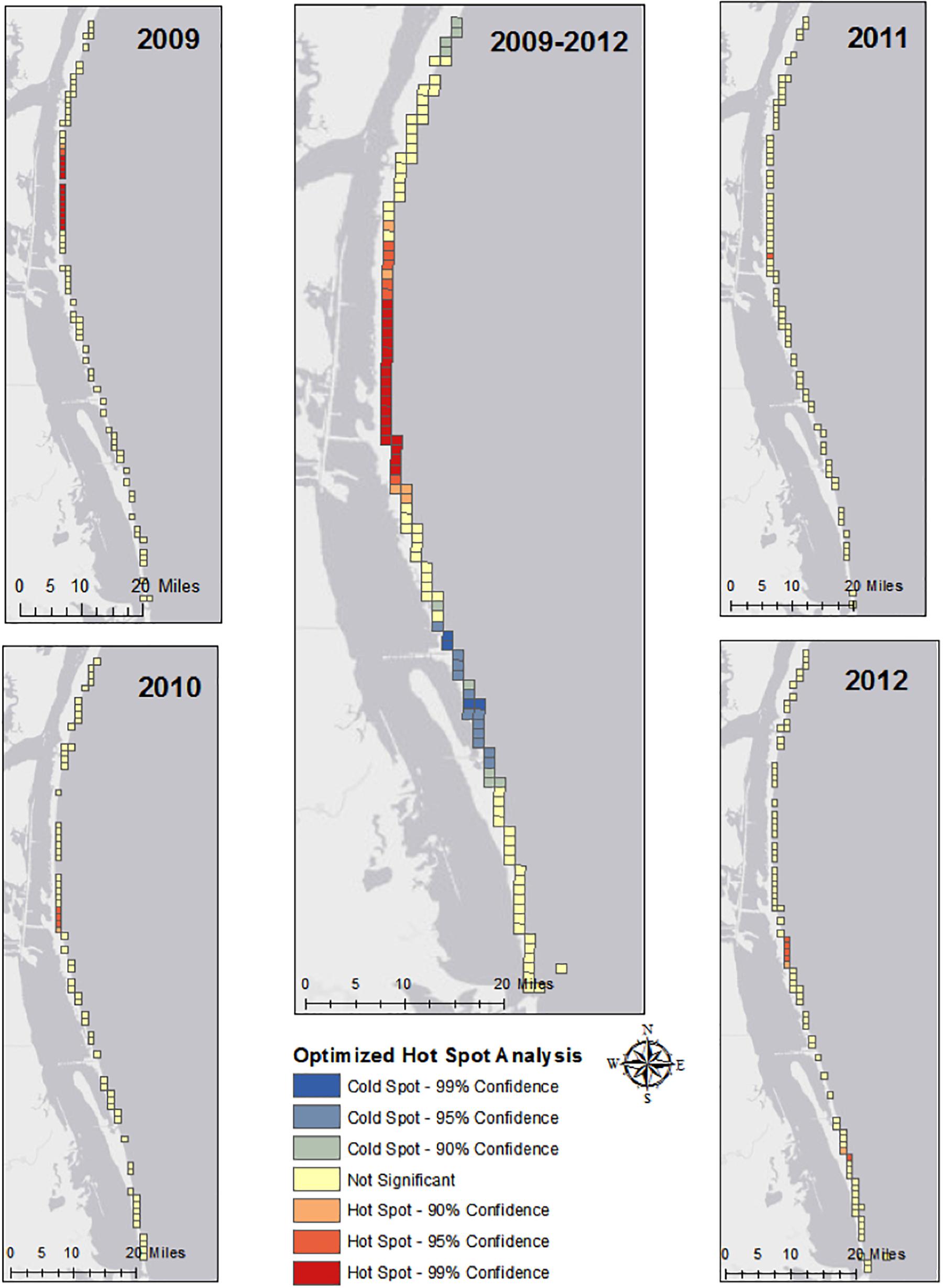
Figure 2. Statistically significant hot spots and cold spots for each year of data produced using the Optimized Hot Spot Analysis tool in ArcGIS.

Boxplots of each geomorphology characteristic differentiated by nest presence contrast the range of geomorphology values used by the Kemp’s ridley sea turtle with the total range of available nesting area (Supplementary Figures 1–7). For most of the geomorphology characteristics, the extent used by the Kemp’s ridley for nesting is limited in comparison to the breadth of the entire study area; the Kemp’s ridley tends to avoid extreme values. The median value for presence points is lower than the median value for the background points for the variables elevation, distance from shoreline, maximum dune slope, dune width, and average beach slope. In particular, the interquartile range of the presence points does not overlap with the interquartile range of the background data for elevation and distance from shoreline, indicative of a distinct preference of the species.

Furthermore, Table 2 lists statistical measures of each geomorphology characteristic for the nest coordinates for all years of data combined, which provides a detailed quantification of the terrestrial habitat range of the Kemp’s ridley sea turtle.

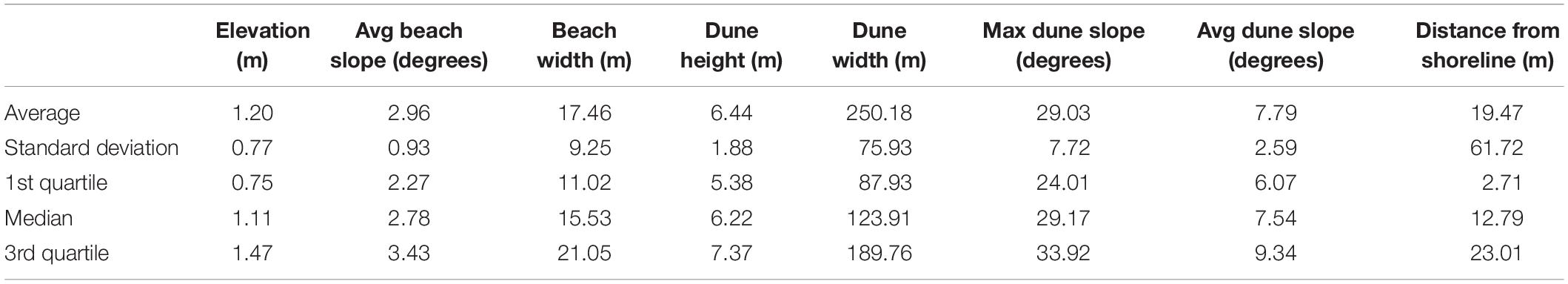
Table 2. Statistical measures of each geomorphology characteristic for the nest coordinates of all of the years of data combined.

Generalized Linear Models

A correlation matrix of the variables revealed collinearity between the following pairs of variables: maximum dune slope and average dune slope, maximum beach slope and average beach slope, and elevation and rugosity (Supplementary Figure 8). There was also a notable relationship between elevation and dune height, as well as between elevation and distance from shoreline. Therefore, these pairs of variables were not included in the generalized linear models in order to avoid creating a bias.

The generalized linear models created using higher ratios of pseudo-absence to presence points had a lower prediction error than models created using a lower ratio (Table 3). However, the results of the confusion matrices of the models created using varying ratios of pseudo-absence to presence points revealed that the ratio acts a factor for model accuracy in predicting pseudo-absence to presence points (Table 3). As the ratio of pseudo-absence to presence points decreases, the accuracy of the predictions for nest presence, or sensitivity, increases and the accuracy of the predictions for nest absence, or specificity, decreases. This is supported by the trends in the boxplots of the predictions of each model differentiated by the observed values (Supplementary Figures 9–14). These boxplots revealed that the median prediction value for the presence points increases in accuracy at a faster rate than the median prediction value for the absence points decreases in accuracy, resulting in a somewhat balanced accuracy in the model created using an equal ratio. Consequently, an equal of pseudo-absence to presence points was determined to be optimal for the purposes of this study because the resulting model was the most accurate in predicting the presence points without exceedingly hindering accuracy in predicting the absence points.

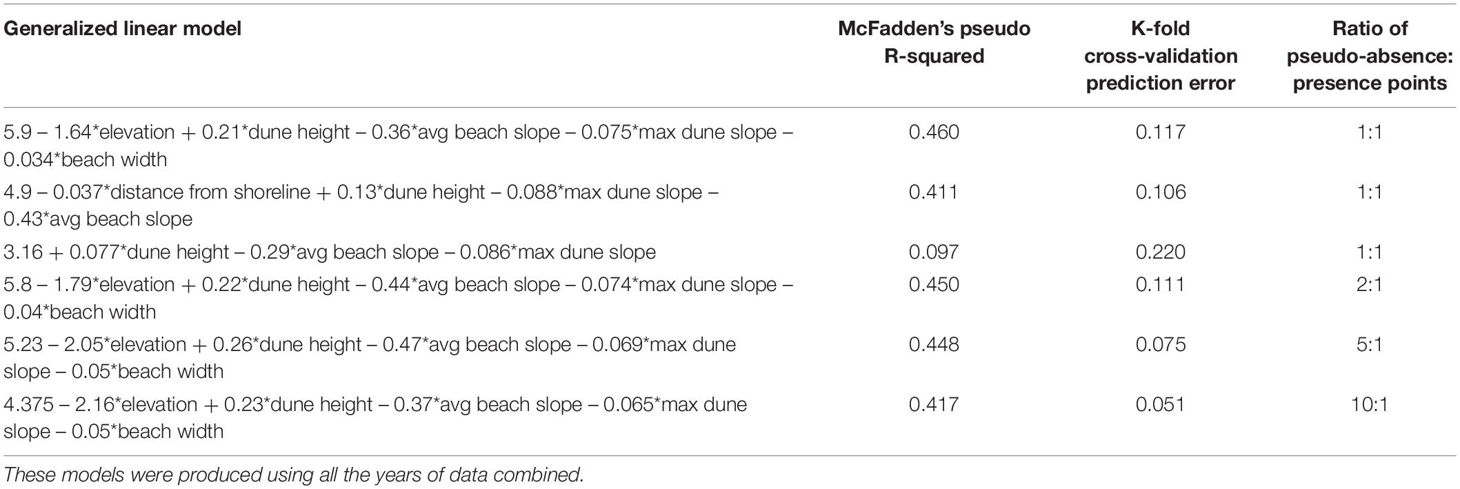
Table 3. Generalized linear models created using varying ratios of pseudo-absence to presence points and their respective measures of accuracy.

Generalized linear models generated using an equal ratio of pseudo-absence to presence points explained 40–46% of the variability of nest presence with a relatively low prediction error (Table 3). In each model, each variable was significant with a p-value < 0.001. The top two models both contained the variables elevation and distance from shoreline, which are collinear. Additionally, these models included the variables of dune height, average beach slope, and maximum dune slope as well. A model containing the aforementioned significant variables without elevation or distance from shoreline only had a pseudo R-squared value of 0.097, indicative that the variables elevation and distance from shoreline are the most influential for the top two models (Table 3). Response curves of the predictions of models 1 and 2 in Table 3 show the relationship between the probability of nest presence and elevation and distance from shoreline, respectively (Figures 3, 4).

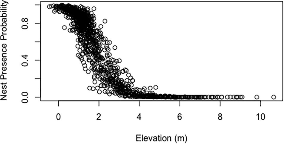
Figure 3. Response curve of the predictions of model 1 in Table 3 showing the probability of nest presence versus elevation (m).

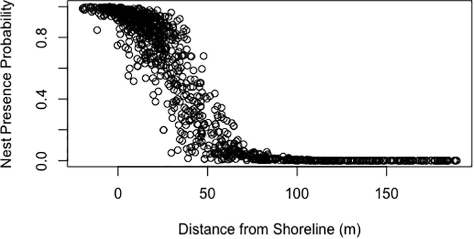
Figure 4. Response curve of the predictions of model 2 in Table 3 showing the probability of nest presence versus distance from shoreline (m).

The spline correlogram of the raw data for all years of data combined revealed positive spatial autocorrelation between nests up to 250 m apart (Supplementary Figure 15). However, the spline correlogram of the Pearson residuals of the top generalized linear model for all the years combined (first model in Table 4) exhibited little spatial autocorrelation between nests, even within a short distance (Supplementary Figure 16). This suggests that the spatial autocorrelation in the data was explained by the explanatory variables in the model (Zuur et al., 2009; Crase et al., 2014). Therefore, the generalized linear model does not need to be adapted to account for spatial autocorrelation (Zuur et al., 2009).

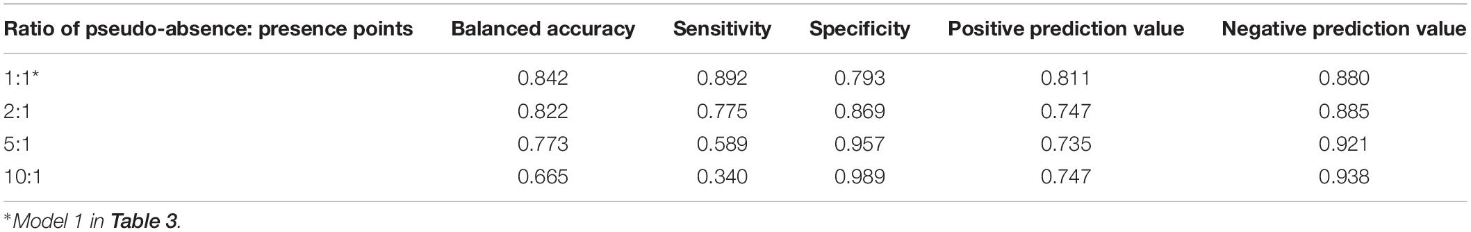
Table 4. Results of the confusion matrices for GLMs created using varying ratios of pseudo-absence to presence points.

Random Forest

The random forest model generated using an equal ratio of pseudo-absence to presence points improved upon the accuracy of the comparable generalized linear models (Table 5). A random forest model was also generated using a 10:1 ratio of pseudo-absence points to presence points, which had a lower sensitivity in comparison to the model created using an equal ratio (Table 5). This is indicative that the higher ratio of pseudo-absence to presence points biases the model against the presence data, which is consistent with the trends between the generalized linear models created using varying ratios of pseudo-absence to presence points.

Table 5. Results of confusion matrices for random forest models generated using varying ratios of pseudo-absence to presence points.

The receiving operating characteristic (ROC) curve, which shows the false positive rate versus the true positive rate, of the random forest model created using an equal ratio of pseudo-absence to presence points further demonstrates the accuracy of this model (Figure 5). The closer the false positive rate is to 0 and the closer the true positive rate is to 1, the more accurate the model. Therefore, the top random forest model for this study was the model created using an equal ratio of pseudo-absence to presence points. The variable importance plots of this model revealed elevation and distance from shoreline to be the most important variables, concurrent with the results of the generalized linear models (Figure 6).

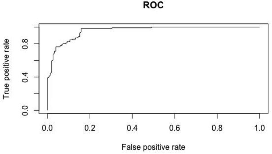
Figure 5. Receiver operating characteristic (ROC) curve of the random forest model.

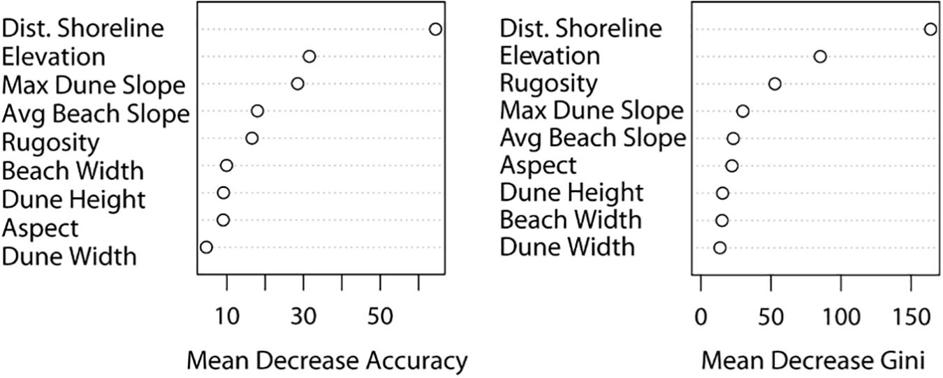
Figure 6. Variable importance plots of the top random forest model. The figure on the left shows the mean decrease in accuracy of the model due to the exclusion of each variable and the figure on the right shows the relative importance of each variable.

Discussion

Kemp’s ridley nest presence was successfully modeled using a small number of geomorphology characteristics, suggestive that these characteristics may be important factors in Kemp’s nest site selection. The top generalized linear models were able to explain 40–46% of the variability of nest presence with a relatively low prediction error (Table 4), and the final random forest model was highly accurate with a true positive rate above 85% (Table 5). The random forest model was superior in performance compared to the generalized linear models, which is indicative of a more complex relationship between nest site selection and beach geomorphology characteristics than can be captured in a traditional modeling technique. This indicates that ranges of the geomorphology characteristics may be more important for Kemp’s ridley nesting than linear trends.

For both the random forest model and the top generalized linear models, elevation and distance from shoreline were the most important variables, but maximum dune slope, dune height, and average beach slope were relatively important variables as well. The importance of elevation and distance from shoreline strongly corresponds to the results of studies regarding both hawksbill and loggerhead sea turtles. Horrocks and Scott (1991); Wood and Bjorndal (2000), Weishampel et al. (2003), and Katselidis et al. (2013) found that the hawksbill and loggerhead prefer to nest at a certain elevation above mean sea level. Furthermore, Dunkin et al. (2016) developed a model that successfully predicted loggerhead habitat suitability using geomorphology characteristics, of which elevation proved to be the most influential factor. Multiple studies also found beach slope characteristics are an important factor for other sea turtle species in locating suitable nesting habitat (Kolbe and Janzen, 2002; Tucker, 2010; Katselidis et al., 2013).

Results showed that Kemp’s ridleys nest at a median elevation of 1.04 m above mean sea level and a median distance from shoreline of 12.79 m, which corresponds to the area near the potential vegetation line or the lowest elevation dune vegetation may thrive along the Texas Gulf shore (Table 2). These findings are consistent with the species description by Marquez-M (1994) that the Kemp’s ridley usually nests in front of the first dune, on the windward slope, or on top of the dune. A comparison of the ranges of values of geomorphology characteristics for the beaches at which Kemp’s ridleys nested to the ranges for the entire study area revealed that Kemp’s ridleys exhibited a preference for a limited range of the available habitat and avoided nesting on beaches with extreme values for maximum dune slope, average beach slope, and beach width. Additionally, for each geomorphology characteristic, nesting occurred at a median value that is lower than the median value for the pseudo-absence points, suggestive of an aversion to maximum values of geomorphology characteristics. This coincides with trends exhibited by other species. Yamamoto et al. (2012) documented that the loggerhead, green, and leatherback sea turtles each exhibited tolerances for a range of values of geomorphology characteristics and would not nest on beaches with values outside these tolerances.

Figure 7 shows examples of profiles that would not be preferred for nesting because they are characterized by extreme values for the beach geomorphology characteristics. On the other hand, Figure 8 shows examples of profiles that would be preferred for nesting because they are characterized by beaches with moderate widths and slopes, as well as prominent foredune complexes.

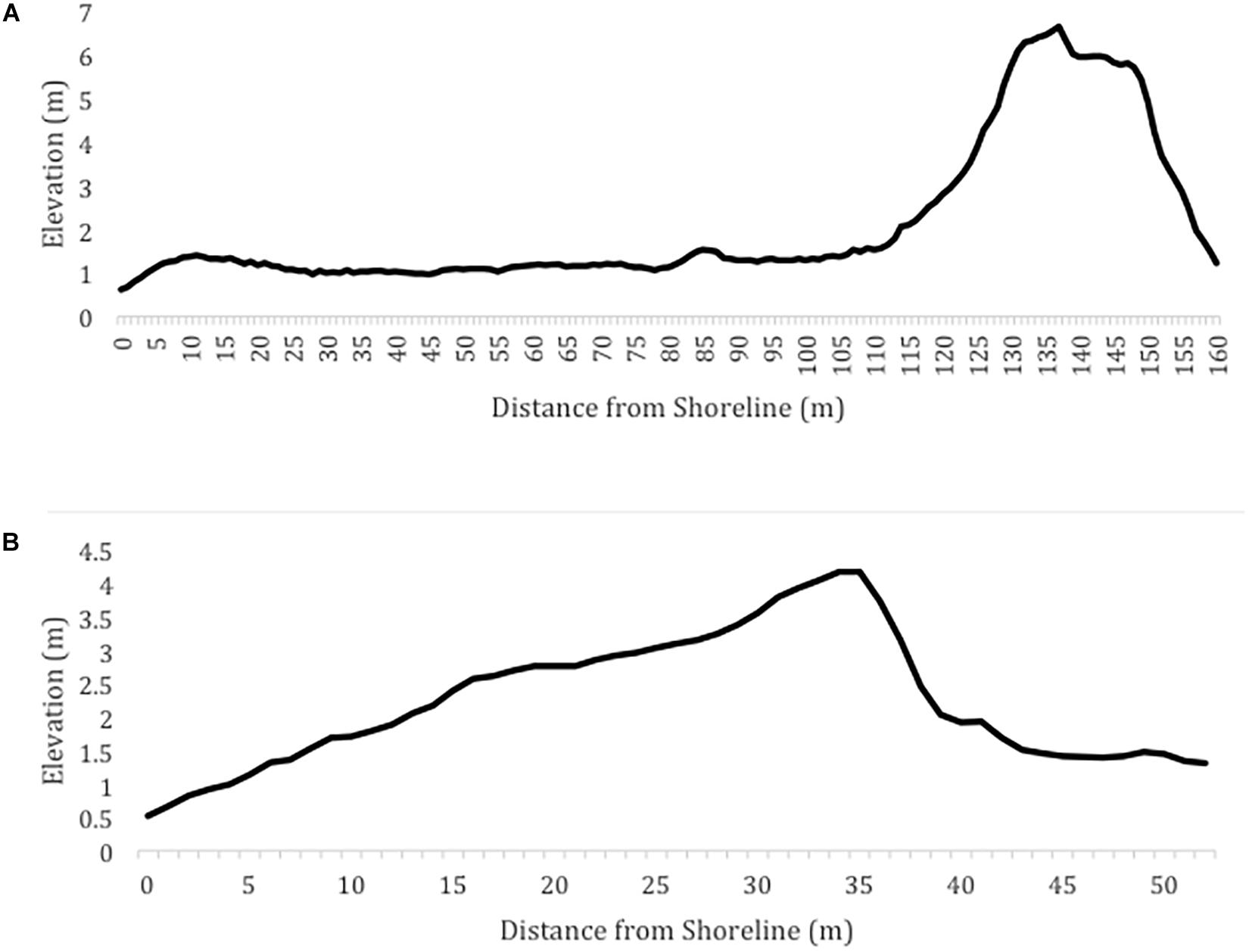
Figure 7. Examples of beach profiles that would not be preferred for nesting due to (A) the wide, flat beach and (B) the narrow, steep beach and high average dune slope.

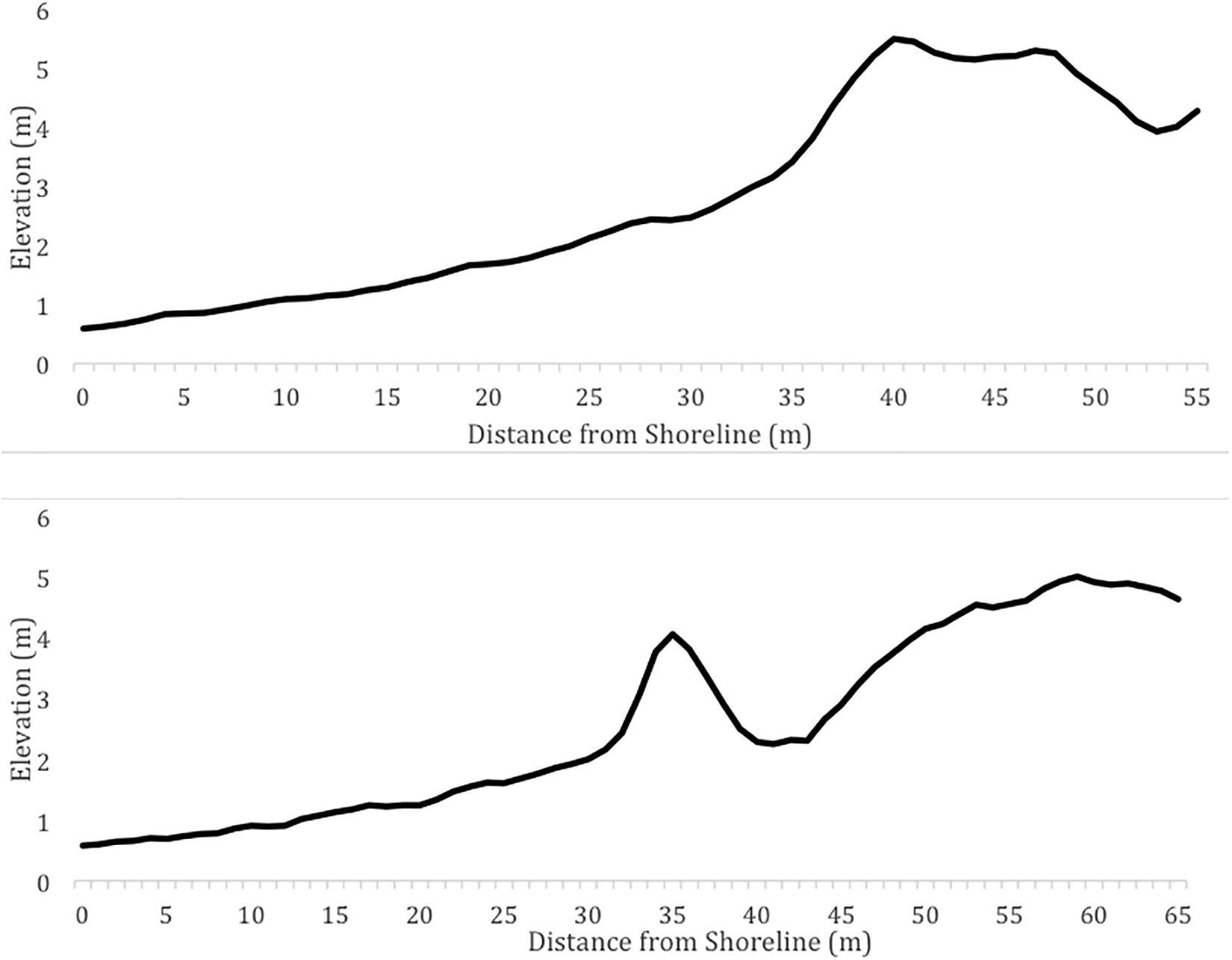
Figure 8. Example of profiles that would be preferred for nesting due to the moderate beach slope and width and prominent dune complex.

Spatially, Kemp’s ridleys nested at a higher frequency in a hot spot along the central section of the study area (Figure 2). The beaches in this region are on average narrower, steeper and characterized by higher dune peaks in comparison to the northern sections of the study area. The beaches in this region of the study area resemble the beaches of Rancho Nuevo, Mexico, the main nesting site of the Kemp’s ridley (Carranza-Edwards et al., 2004). Both regions are also characterized by the presence of shell fragments (Carranza-Edwards et al., 2004; National Marine Fisheries Service [NMFS] et al., 2010; National Marine Fisheries Service and U. S. Fish and Wildlife Service, 2015).

The models did not explain all of the variability in Kemp’s ridley nest presence, indicative that other factors, such as coastal development, alongshore currents, offshore bathymetry, sediment size, or environmental conditions, could also be influential (Weishampel et al., 2003; Pike, 2008; Garcon et al., 2010; Katselidis et al., 2013; Thums et al., 2019). Kemp’s ridleys often nest in synchronous emergences called arribadas, and studies suggest that there may be cues that initiate an arribada, including strong onshore wind, lunar and tidal cycles, olfactory signals, or social facilitation (Shaver and Rubio, 2008; Shaver et al., 2017). Jimenez-Quiroz et al. (2005) found a coherence between nesting cycles and temperature and wind fluctuations, implying that these environmental variables could serve as stimuli for nesting. Shaver et al. (2017) discerned that Kemp’s ridleys prefer to nest on windy days and may be prompted to nest by increases in wind speed and surf. It is possible that these conditions are preferable because the sand is cooler and the risk of predation is reduced, as any signs of nesting would be quickly erased (Shaver et al., 2017). Similarly, multiple studies regarding other species of sea turtles indicate that environmental factors, such as wind and wave exposure, oceanic currents, rainfall events, and tide levels, may be related to sea turtle nest site selection (Pike, 2008; Garcon et al., 2010; Thums et al., 2019). Future modeling efforts should attempt to strengthen the predictions for Kemp’s ridley nest site selection by incorporating these environmental drivers.

Kemp’s Ridley Conservation and Management

There are a variety of species management and conservation applications for the results of this study that would help protect the Kemp’s ridley sea turtle and its habitat. The methods developed in this study can be used to monitor and protect Kemp’s ridley habitat availability along the Texas coast as both human (i.e., beach nourishment and beach maintenance) and natural processes (i.e., sea-level rise and extreme storm events) alter beach geomorphology characteristics.

Beach nourishment projects are often a necessary source protection against shoreline erosion, but beach nourishment and beach maintenance activities can result in changes to beach characteristics that may be important for sea turtle nesting, such as beach slope and width, sand compaction, gaseous environment, hydric environment, containment levels, nutrient availability, and thermal environment (Crain et al., 1995; Gallaher, 2009). This could result in a decrease in sea turtle nesting habitat suitability and may deter nesting. Resource managers and city planners can use the results of this study to limit degradation to Kemp’s ridley terrestrial habitat during beach nourishment and maintenance projects by ensuring the geomorphology characteristics of all managed beaches fall within the habitat range of the species. Specifically, this data can be used to help generate a habitat suitability index for the Kemp’s ridley to be considered during the permitting process.

The results of this study can also be expanded upon to calculate the extent of nesting habitat that may be at risk to sea-level rise and identify beaches where nesting may shift. Sea-level rise has the potential to cause an increase in nest inundation events and to change beach geomorphology characteristics key to sea turtle nesting, such as beach slope and elevation (Pendleton et al., 2004; Stutz and Pilkey, 2011; Williams, 2013; Santos et al., 2015). Annual and seasonal measurements of beach geomorphology characteristics could be used to calculate how the morphology of nesting beaches is changing and to predict the extent and location of optimal nesting habitat as the beaches continue to shift (Katselidis et al., 2013).

The results of this study can also be applied to Kemp’s ridley nest location efforts. Because Kemp’s ridleys are a relatively small and light sea turtle species, they leave only a faint track in the sand, rendering it especially difficult for nest chambers to be located on windy days. During windy conditions, searches for Kemp’s ridley nests should be focused on areas where Kemp’s ridleys are most likely to nest, such as near the potential line of vegetation and along the central section of North Padre Island, Texas within the Padre Island National Seashore.

Conclusion

This is the first study to assess the relationship between beach geomorphology characteristics and nest site selection for the Kemp’s ridley, the most endangered sea turtle species in the world. This research serves as an example of how remote sensing data can be used to model wildlife habitat over an expansive study area and obtain detailed information about an endangered species that is difficult to study.

The application of high-resolution lidar data resulted in new information regarding the terrestrial habitat variability and nesting preferences of the Kemp’s ridley sea turtle, which can be used to benefit the conservation and management of the species. Although other factors may influence beach selection by the Kemp’s, beach geomorphology characteristics were able to be used to predict nest presence. This is suggestive of a degree of importance of geomorphology characteristics in Kemp’s nest site selection, which coincides with similar studies regarding other species. Nevertheless, future work should focus on generating a more robust model that incorporates other potential factors, such as the presence of vegetation, human activity, or sand characteristics, in hopes of explaining more of the variability of Kemp’s ridley nest presence.

Data Availability Statement

The datasets for this study have been submitted to Gulf of Mexico Research Initiative Information and Data Cooperative, and publicly available at: https://data.gulfresearchinitiative.org/data/HI.x833.000:0002 (10.7266/N7445K0Z).

Author Contributions

JG, DS, MS, PT, and MC conceptualized the study. DS contributed the nest coordinates. MC, JG, and PT performed the data analysis. MC wrote the manuscript with contributions from DS, JG, MS, and PT.

Funding

This work was supported by the Crutchfield Fellowship at the Harte Research Institute for Gulf of Mexico Studies at TAMUCC. This funding source had no involvement in the conduct of the research and/or preparation of the article.

Conflict of Interest

The authors declare that the research was conducted in the absence of any commercial or financial relationships that could be construed as a potential conflict of interest.

Acknowledgments

We would like to thank the Harte Research Institute for Gulf of Mexico Studies and the Padre Island National Seashore Sea Turtle Division for their support.

Supplementary Material

The Supplementary Material for this article can be found online at: https://www.frontiersin.org/articles/10.3389/fmars.2020.00214/full#supplementary-material

References

Barbet-Massin, M., Jiguet, F., Albert, C. H., and Thuiller, W. (2012). Selecting pseudo-absences for species distribution models: how, where and how many? Methods Ecol. Evol. 3, 327–338. doi: 10.1111/j.2041-210x.2011.00172.x
Caillouet, C. W., Shaver, D. J., and Landry, A. M. (2015). Kemp’s ridley sea turtle (Lepidochelys kempii) head-start and reintroduction to padre island national seashore, Texas. ResearchGate 10, 309–377.
Carranza-Edwards, A., Rosales-Hoz, L., Chávez, M. C., and de la Garza, E. M. (2004). “Environmental geology of the coastal zone,” in Environmental Analysis of the Gulf of Mexico, eds M. Caso, I. Pisanty, and E. Ezcurra (College Station, TX: Texas A&M University Press), 351–372.
Crain, D. A., Bolten, A. B., and Bjorndal, K. A. (1995). Effects of Beach nourishment on sea turtles: review and research initiatives. Restorat. Ecol. 3, 95–104. doi: 10.1111/j.1526-100X.1995.tb00082.x
Crase, B., Liedloff, A., Vesk, P. A., Fukuda, Y., and Wintle, B. A. (2014). Incorporating spatial autocorrelation into species distribution models alters forecasts of climate-mediated range shifts. Glob. Chang. Biol. 20, 2566–2579. doi: 10.1111/gcb.12598
Cuevas, E., Liceaga-Correa, M. Á, and Mariño-Tapia, I. (2010). Influence of Beach slope and width on hawksbill (Eretmochelys imbricata) and green turtle (Chelonia mydas) nesting activity in El Cuyo, Yucatán, Mexico. Chelonian Conserv. Biol. 9, 262–267. doi: 10.2744/ccb-0819.1
Davis, R. A. (1977). Beach sedimentology of Mustang and Padre Islands: a time-series approach. J. Geol. 86, 35–46. doi: 10.1086/649654
Dormann, C. F., McPherson, J. M., Araújo, M. B., Bivand, R., Bolliger, J., Carl, G., et al. (2007). Methods to account for spatial autocorrelation in the analysis of species distributional data: a review. Ecography 30, 609–628. doi: 10.1111/j.2007.0906-7590.05171.x
Dunkin, L., Reif, M., Altman, S., and Swannack, T. (2016). A spatially explicit, multi-criteria decision support model for loggerhead sea turtle nesting habitat suitability: a remote sensing-based approach. Remote Sens. 8:573. doi: 10.3390/rs8070573
Elith, J., Graham, C. H., Anderson, R. P., Dudík, M., Ferrier, S., Guisan, A., et al. (2006). Novel methods improve prediction of species’ distributions from occurrence data. Ecography 29, 129–151.
Gallaher, A. A. (2009). The Effects of Beach Nourishment on Sea Turtle Nesting Densities in Florida. Ph.D. thesis, University of Florida, Florida, IL.
Garcon, J. S., Grech, A., Moloney, J., and Hamann, M. (2010). Relative exposure index: an important factor in sea turtle nesting distribution. Aquat. Conserv. 20, 140–149. doi: 10.1002/aqc.1057
Gibeaut, J. C., and Caudle, T. (2009). Defining and Mapping Foredunes, the Line of Vegetaiton, and Shorelines along the Texas Gulf Coast. Corpus Christ, TX: Harte Research Institute for Gulf of Mexico Studies at TAMU-CC.
Gibeaut, J. C., Gutiérrez, R., and Hepner, T. L. (2002). Threshold conditions for episodic beach erosion along the southeast Texas coast. Gulf Coast Assoc. Geol. Soc. Trans. 52, 323–335.
Gilmour, A. R., Anderson, R. D., and Rae, A. L. (1985). The analysis of binomial data by generalized linear mixed model. Biometrika 72, 593–599. doi: 10.1093/biomet/72.3.593
Horrocks, J. A., and Scott, N. M. (1991). Nest site location and nest success in the hawksbill turtle Eretmochelys imbricata in Barbados, West Indies. Mar. Ecol. Prog. Ser. 69, 1–8. doi: 10.3354/meps069001
Jimenez-Quiroz, M., del, C., Filonov, A., Tereshchenko, I., and Marquez-Milan, R. (2005). Time-series analyses of relationship between nesting frequency of the Kemp’s ridley sea turtle and meterological conditions. Chelonian Conserv. Biol. 2005, 774–780.
Judd, F. W., Lonard, R. I., and Sides, S. L. (1977). The vegetation of South Padre Island, Texas in relation to topography. Southw. Nat. 22, 31–48.
Katselidis, K. A., Schofield, G., Dimopoulous, G. S. P., and Pantis, J. D. (2013). Evidence based management to regulate the impact of tourism at a key sea turtle rookery. Oryx 47, 584–594. doi: 10.1017/S0030605312000385
Kolbe, J. J., and Janzen, F. J. (2002). Impact of nest-site selection on nest success and nest temperature in natural and disturbed habitats. Ecology 83, 269–281. doi: 10.1890/0012-9658(2002)083[0269:ionsso]2.0.co;2
Marquez-M, R. (1994). Synopsis of Biological Data on the Kemp’s Ridley Turtle, Lepidochelys Kempi, (Garman, 1880) (No. NOAA Technical Memorandum NMFS-SEFSC-343). Silver Spring, MD: NOAA.
McFadden, D. (1974). “Conditional logit analysis of qualitative choice behavior,” in Frontiers in Econometrics, ed. P. Zarembka (Cambridge, MA: Academic Press), 105–142.
Mi, C., Huettmann, F., Guo, Y., Han, X., and Wen, L. (2017). Why choose Random Forest to predict rare species distribution with few samples in large undersampled areas? Three Asian crane species models provide supporting evidence. PeerJ 5:e2849. doi: 10.7717/peerj.2849
Mortimer, J. A. (1982). “Factors influencing beach selection by nesting sea turtles,” in Biology and Conservation of Sea Turtles, ed. K. A. Bjorndal (Washington, DC: Smithsonian Institution Press), 45–51.
Mortimer, J. A. (1990). The Influence of Beach Sand Characteristics on the Nesting Behavior and Clutch Survival of Green Turtles (Chelonia mydas). Lawrence: American Society of Ichthyologists and Herpetologists, 802–817.
National Marine Fisheries Service [NMFS] et al. (2010). Draft Bi-National Recovery Plan for the Kemp’s Ridley Sea Turtle, Secon Revision. Silver Spring, MD: National Marine Fisheries Service.
National Marine Fisheries Service, and U. S. Fish and Wildlife Service (2015). Kemp’s Ridley Sea Turtle 5-Year Review: Summary and Evaluation. Silver Spring, MD: NOAA.
Paine, J., Caudle, T., and Andrews, J. (2013). Shoreline, Beach, and Dune Morphodynamics, Texas Gulf Coast (No. 09-242-000-3789). Austin, TX: Bureau of Economic Geology.
Pendleton, E. A., Thieler, E. R., Williams, S. J., and Beavers, R. L. (2004). Coastal Vulnerability Assessment of Padre Island National Seashore (PAIS) to Sea-Level Rise. Reston: U.S. Geological Survey.
Phillips, S. J., Dudík, M., Elith, J., Graham, C. H., Lehmann, A., Leathwick, J., et al. (2009). Sample selection bias and presence-only distribution models: implications for background and pseudo-absence data. Ecol. Appl. 19, 181–197. doi: 10.1890/07-2153.1
Pike, D. A. (2008). Environmental correlates of nesting in loggerhead turtles, Caretta caretta. Anim. Behav. 76, 603–610. doi: 10.1186/s40462-018-0145-1
Provancha, J. A., and Ehrhart, L. M. (1987). “Sea turtle nesting trends at kennedy space center and Cape Canaveral Air Force Station, Florida, and relationships with factors influencing nest-site selection,” in Ecology of East Florida Sea Turtles: Proceedings of the Cape Canaveral, Florida Sea Turtle Workshop Miami, Florida February 26–27, 1985 NOAA Technical Report NMFS 53, ed. W. N. Witzell (Seattle, WA: NOAA), 33–44.
Putman, N. F., Mansfield, K. L., He, R., Shaver, D. J., and Verley, P. (2013). Predicting the distribution of oceanic-stage Kemp’s ridley sea turtles. Biol. Lett. 9:20130345. doi: 10.1098/rsbl.2013.0345
Santos, K. C., Livesey, M., Fish, M., and Lorences, A. C. (2015). Climate change implications for the nest site selection process and subsequent hatching success of a green turtle population. Mitig. Adapt. Strateg. Glob. Chang. 22, 121–135. doi: 10.1007/s11027-015-9668-6
Santos, K. C., Tague, C., Alberts, A. C., and Franklin, J. (2006). Sea turtle nesting habitat on the US Naval station, guantanamo Bay, Cuba: a comparison of habitat suitability index models. Chelonian Conserv. Biol. 5, 175–187. doi: 10.2744/1071-8443(2006)5%5B175:stnhot%5D2.0.co;2
Shaver, D. J., and Caillouet, C. W. Jr. (2015). Reintroduction of Kemp’s ridley (Lepidochelys kempii) sea turtle to padre Island National Seashore, Texas and its connection to head-starting. Herpetol. Conserv. Biol. 10, 378–435.
Shaver, D. J., Hart, K. M., Fujisaki, I., Bucklin, D., Iverson, A. R., and Rubio, C. (2017). Inter-nesting movements and habitat-use of adult female Kemp’s ridley turtles in the Gulf of Mexico. PLoS One 12:e0174248. doi: 10.1371/journal.pone.0174248
Shaver, D. J., and Rubio, C. (2008). Post-nesting movement of wild and head-started Kemp’s ridley sea turtles Lepidochelys kempii in the Gulf of Mexico. Endang. Spec. Res. 4, 43–55. doi: 10.3354/esr00061
Starek Michael, J., Vemula, R., and Slatton, K. C. (2012). Probabilistic detection of morphologic indicators for beach segmentation with multitemporal lidar measurements. IEEE Trans. Geosci. Remote Sens. 50, 1–12.
Stutz, M. L., and Pilkey, O. H. (2011). Open-ocean barrier islands: global influence of climatic, oceanographic, and depositional settings. J. Coast. Res. 27, 207–222. doi: 10.2112/09-1190.1
Svetnik, V., Liaw, A., Tong, C., Culberson, J. C., Sheridan, R. P., and Feuston, B. P. (2003). Random forest: a classification and regression tool for compound classification and QSAR modeling. J. Chem. Inform. Comput. Sci. 43, 1947–1958. doi: 10.1021/ci034160g
Thums, M., Rossendell, J., Fisher, R., and Guinea, M. L. (2019). Nesting ecology of flatback sea turtles (Natator depressus) from Delambre Island, Western Australia. Mar. Freshw. Res. 602, 237–253.
Tucker, A. D. (2010). Nest site fidelity and clutch frequency of loggerhead turtles are better elucidated by satellite telemetry than by nocturnal tagging efforts: implications for stock estimation. J. Exp. Mar. Biol. Ecol. 383, 48–55. doi: 10.1016/j.jembe.2009.11.009
VanDerWal, J., Shoo, L. P., Graham, C., and Williams, S. E. (2009). Selecting pseudo-absence data for presence-only distribution modeling: how far should you stray from what you know? Ecol. Model. 220, 589–594. doi: 10.1016/j.ecolmodel.2008.11.010
Watson, R. T. (1971). Origin of shell beaches, Padre Island, Texas. J. Sedim. Petrol. 41, 1105–1111.
Weise, B. R., and White, W. A. (2007). Padre Island National Seashore: A Guide to the Geology, Natural Environments, and History of a Texas Barrier Island (No. Guidebook 17 Bureau of Economic Geology, University of Texas at Austin). Austin, TX: University of Texas, Bureau of Economic Geology.
Weishampel, J. F., Bagley, D. A., and Ehrhart, L. M. (2006). Intra-annual loggerhead and green turtle spatial Nesting Patterns. Southeast. Nat. 5, 453–462. doi: 10.1656/1528-7092(2006)5%5B453:ilagts%5D2.0.co;2
Weishampel, J. F., Bagley, D. A., Ehrhart, L. M., and Rodenbeck, B. L. (2003). Spatiotemporal patterns of annual sea turtle nesting behaviors along an east central Florida beach. Biol. Conserv. 110, 295–303. doi: 10.1016/s0006-3207(02)00232-x
Williams, S. J. (2013). Sea-level rise implications for coastal regions. J. Coast. Res. 63, 184–196. doi: 10.2112/SI63-015.1
Wood, D. W., and Bjorndal, K. A. (2000). Relation of temperature, moisture, salinity, and slope to nest site selection in loggerhead Sea Turtles. Am. Soc. Ichthyol. Herpetol. Copeia 1, 119–128.
Yamamoto, K. H., Powell, R. L., Anderson, S., and Sutton, P. C. (2012). Using Lidar to quantify topographic and bathymetric details for sea turtle nesting beaches in Florida. Remote Sens. Environ. 125, 125–133. doi: 10.1016/j.rse.2012.07.016
Zavaleta-Lizárraga, L., and Morales-Mávil, J. E. (2013). Nest site selection by the green turtle (Chelonia mydas) in a beach of the north of Veracruz, Mexico. Rev. Mexic. Biodivers. 84, 927–937. doi: 10.7550/rmb.31913
Keywords: sea turtle, lidar data, habitat model, coastal, beach geomorphology
Citation: Culver M, Gibeaut JC, Shaver DJ, Tissot P and Starek M (2020) Using Lidar Data to Assess the Relationship Between Beach Geomorphology and Kemp’s Ridley (Lepidochelys kempii) Nest Site Selection Along Padre Island, TX, United States. Front. Mar. Sci. 7:214. doi: 10.3389/fmars.2020.00214
Received: 31 January 2020; Accepted: 19 March 2020;
Published: 08 April 2020.
Edited by:
Michele Thums, Australian Institute of Marine Science (AIMS), AustraliaReviewed by:
Vinay Udyawer, Australian Institute of Marine Science (AIMS), AustraliaGail Schofield, Queen Mary University of London, United Kingdom
Copyright © 2020 Culver, Gibeaut, Shaver, Tissot and Starek. This is an open-access article distributed under the terms of the Creative Commons Attribution License (CC BY). The use, distribution or reproduction in other forums is permitted, provided the original author(s) and the copyright owner(s) are credited and that the original publication in this journal is cited, in accordance with accepted academic practice. No use, distribution or reproduction is permitted which does not comply with these terms.
*Correspondence: Michelle Culver, michellefculv@gmail.com