Ensemble Projections of Future Climate Change Impacts on the Eastern Bering Sea Food Web Using a Multispecies Size Spectrum Model

Introduction

Anthropogenic climate change is expected to have significant impacts on ocean biogeochemistry, primary and secondary production, and the distribution and productivity of higher trophic level species (Doney et al., 2012; Mora et al., 2013; Pecl et al., 2017). Given the complexity and large spatiotemporal scales at which marine ecosystems operate, modeling approaches are necessary for inferring possible outcomes and tradeoffs due to climate change. For large marine ecosystems, models of varying complexity have been used to project potential impacts on community structure, size composition, and fishery catches, and to evaluate management strategies under climate change (e.g. Niiranen et al., 2013; Barange et al., 2014; Marshall et al., 2017). However, efforts to quantify uncertainty in climate-forced ecological projections have lagged, which limits their utility for informing ecosystem approaches to management and decision-making (Payne et al., 2015; Cheung et al., 2016).

Ensemble modeling enables representation of multiple sources of uncertainty. The approach entails developing a set of models, with each model member representing different working hypotheses or alternative formulations of uncertain processes. For instance, regional studies have evaluated structural uncertainty using model ensembles that consist of different formulations of species interactions (Gårdmark et al., 2013) or biogeochemical processes (MacKenzie et al., 2012; Meier et al., 2012; Niiranen et al., 2013). However, climate-forced ecological projections also depend on assumptions regarding future socio-economic policies, markets, or technological developments that result in different greenhouse gas (GHG) emissions scenarios (Payne et al., 2015; Cheung et al., 2016). For specific marine ecosystems, scenario uncertainty could also encompass implementations of different policies, for instance, that impact fisheries regulations or coastal land use patterns. The distribution of projected outcomes conveys the level of confidence conditional on the set of alternative future scenarios and the model ensemble. Moreover, the uncertainty can be partitioned according to source which helps characterize their relative influence on the projection spread and informs where gains in precision may be made, for instance, through model refinement, additional research and observations, or advances in theory (Hawkins and Sutton, 2009; Cheung et al., 2016). Ensemble modeling is now widely used in weather and climate forecasting (e.g. Murphy et al., 2004; Berliner and Kim, 2008), but remains underutilized with respect to climate-driven ecosystem projections (Cheung et al., 2016).

Mechanistic food web models offer a powerful framework for exploring potential tradeoffs and uncertainties under different environmental or management scenarios (Persson et al., 2014). In marine and freshwater ecosystems, predation interactions are strongly size-structured and size-based food web models offer a relatively simple way to capture key aspects of system dynamics (Kerr and Dickie, 2001; Andersen et al., 2016; Guiet et al., 2016; Blanchard et al., 2017). Size spectra depict the abundance of individuals as a continuous function of body mass, and the first dynamic size spectrum models were developed to explain regularities observed in the scaling of abundance with body mass in lake and ocean ecosystems [reviewed in Blanchard et al. (2017)]. In size spectra models, system dynamics emerge from rules regarding the prey size preference of predators and the allocation of ingested energy toward maintenance costs, growth, and reproduction. The models are effective at capturing large-scale patterns in fisheries production despite their simplicity, and can be forced with Earth System Model (ESM) outputs to project future community size structure and bulk fisheries production (Blanchard et al., 2012; Woodworth-Jefcoats et al., 2013; Barange et al., 2014; Lefort et al., 2015). Recent extensions to the modeling framework, however, permit explicit representation of multiple interacting species and their fisheries (Andersen et al., 2016; Blanchard et al., 2017). Species can be distinguished according to life history and prey size and species preference and predation, growth, and reproduction are represented at the individual-level using a dynamic energy budget framework (Hartvig et al., 2011; Blanchard et al., 2014; Andersen et al., 2016). This latter feature makes multispecies size spectrum models (MSSMs) strong candidates for evaluating climate impacts because the hypothesized effects of climate variables (e.g. temperature) on animal energy budgets can be modeled in a more mechanistic fashion and scaled up to the population and community levels (Maury and Poggiale, 2013; Lefort et al., 2015; Guiet et al., 2016; Woodworth-Jefcoats et al., 2019).

Here, we evaluated future climate impacts on the eastern Bering Sea (EBS) food web using an MSSM and ensemble modeling approach (Figure 1). The EBS is a highly productive, semi-enclosed subpolar sea that overlays a broad continental shelf (average width ∼500 km). Although physical and biological conditions in the EBS are characterized by high interannual variation (Stabeno et al., 2001), climate change is expected to have multiple impacts. Warmer conditions are expected to reduce the southern spatial extent and duration of seasonal sea ice cover, advance the spring transition, and increase water column stratification, which may negatively impact phytoplankton, zooplankton, and benthic production (Hermann et al., 2013, 2016, 2019). Among global-scale simulation studies of climate change impacts, projections for the EBS are inconsistent and include forecasts of increased total catch potential (Cheung et al., 2010), negligible shifts in pelagic fish biomass (Lefort et al., 2015), and moderate reductions in total fish biomass (Lotze et al., 2018). However, out of practical necessity these studies lack taxonomic detail, make simplifying assumptions regarding growth potential and trophic structure, and are forced with ESM projections with coarse spatial resolution. To better understand the implications of climate change for higher trophic level species and their fisheries in the EBS, the interdisciplinary Alaska Climate Integrated Modeling project (ACLIM) was initiated by the NOAA Alaska Fisheries Science Center (Hollowed et al., 2019). As a component of ACLIM, capacity to dynamically downscale ESM projections to the EBS was expanded (Hermann et al., 2019) and an MSSM was developed for and calibrated to the EBS (Reum et al., 2019).

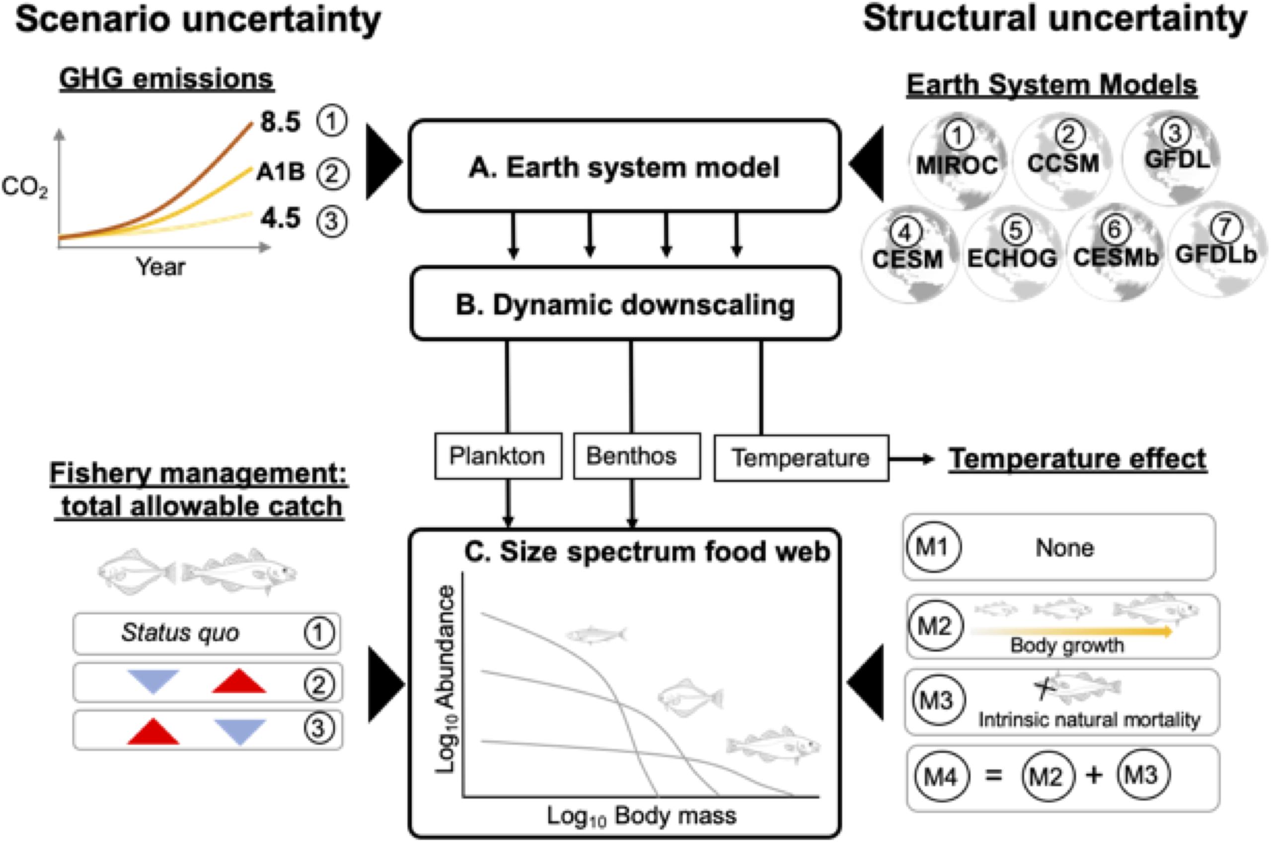
Figure 1. Overview of modeling framework that links outputs from three model levels (A–C) to generate future projections of the eastern Bering Sea food web while incorporating different sources of uncertainty. (A) Multiple Earth System Models (ESMs) were forced under low (RCP 4.5), medium (SRES A1B), and high (RCP 8.5) future greenhouse gas emissions (GHG) scenarios. The ESM projections, in turn, were dynamically downscaled using (B) a regional biophysical model. Projections of temperature and plankton and benthos biomass were used to force (C) a multispecies size spectrum model. Structural uncertainty in projections arise from variability in model forcing parameters related to the different ESMs and hypotheses regarding temperature-dependences on body growth and mortality rates. Scenario uncertainty arises from different future GHG emission and fishery management scenarios that differ with respect to allocation of total allowable catch between flatfish and gadid stocks.

In this study, we built upon these advances and produced ensemble projections of the EBS food web that incorporated multiple sources of uncertainty (Figure 1). Specifically, we included two sources of structural uncertainty (Figure 1). First, down-scaled climate projections for the EBS differ across ESMs (Hermann et al., 2019). We therefore used downscaled climate projections from multiple ESMs. Second, we addressed structural uncertainty related to possible temperature-dependences in biological rates. Temperature influences metabolism, which may impact multiple processes including physiological rates that affect body growth (Kooijman, 2000; Brown et al., 2004) as well as “intrinsic” or non-predation natural mortality (i.e. disease, senescence rates; Munch and Salinas, 2009; Keil et al., 2015). Previous size-based studies have included temperature-dependencies on both body growth-related and intrinsic natural mortality rates (Blanchard et al., 2012; Woodworth-Jefcoats et al., 2013; Lefort et al., 2015), but biological rates can exhibit different scaling relationships with temperature (e.g. Englund et al., 2011; Brown et al., 2004; Rall et al., 2012) and it remains unclear to what degree these two processes influence emergent features of the food web. To account for this uncertainty, we considered multiple MSSM variants that differed with regard to how temperature affects key biological rates (Figure 1). We also included two sources of scenario uncertainty. The first relates to different scenarios of future GHG emissions (Payne et al., 2015; Cheung et al., 2016). The second corresponds to different fisheries management scenarios that, relative to status quo, prioritize fishing on different components of the EBS food web and reflect trade-offs fishery managers are confronted with in setting total allowable catches for each stock (Figure 1; Hollowed et al., 2019).

Our main objectives were to: (1) develop ensemble projections of fish and invertebrate community composition and size structure and partition projection uncertainties according to source over various time horizons and (2) evaluate how different sources of uncertainty interact. For the latter objective, we specifically sought to clarify how policy and decision-making at regional and intergovernmental scales interact by comparing catches and community composition under alternative fishery management scenarios and either business-as-usual or mitigation GHG emissions scenarios. Further, we evaluated how temperature-dependencies operating on individual-level processes related to body growth and intrinsic natural mortality influenced emergent community- and species-level projections and whether their combined effects were additive or not (e.g. Crain et al., 2008; Kaplan et al., 2013).

Materials and Methods

Overview of Modeling Approach

Our modeling framework included three components, each of which supplied outputs that flowed unidirectionally to the next component (Figure 1). The first component (A) consisted of IPCC-class ESMs forced using various GHG emission scenarios based on IPCC Representative Concentration Pathways (R). In the second component (B), ESM projections were dynamically downscaled to the EBS. Specifically, the ESM projections provided boundary conditions for a 10 km spatial resolution regional biophysical model (Hermann et al., 2016, 2019). In the third component (C), a MSSM was forced using dynamically downscaled temperatures and values for phytoplankton, zooplankton, and benthos standing stock from B. Four versions of the MSSM were used in the ensemble to evaluate alternative assumptions regarding temperature-dependencies on biological processes. Aspects of structural uncertainty were accounted for at the ESM and MSSM components (Figure 1), and the model ensemble consisted of all possible combinations of ESMs and MSSMs. Next, we provide an overview of the climate downscaling approach and MSSM implementation. Additional details of the MSSM equations, parameterization, and calibration are available in Reum et al. (2019) and Supplementary Appendix I; details regarding the biophysical model are available in Hermann et al. (2016) and Hermann et al. (2019).

A and B: Earth System Models and Dynamic Downscaling of Climate

Due to the computational demands of dynamically downscaling regional climate projections, we assembled an “ensemble of opportunity” (e.g. Tebaldi and Knutti, 2007) that consisted of two sets of previously published downscaled projections from ESMs and GHG emissions scenarios used in the Intergovernmental Panel on Climate Change Assessment Reports (IPCC AR4 and AR5) and archived by the Coupled Model Inter-comparison Project (CMIP) (Hermann et al., 2016, 2019).

The first set of ESMs included downscaled projections from three ESMs. These included the Coupled Global Climate Model, T47 grid (CGCM3-t4) from the Canadian Centre for Climate Modeling and Analysis, the Hamburg Atmosphere-Ocean Coupled Circulation Model (ECHO-G), and the Model for Interdisciplinary Research on Climate, medium-resolution version (MIROC3.2-Medres; Hermann et al., 2016). We refer to these ESMs as CGCM, ECHO, and MIROC, respectively. All ESM outputs from this set were archived by CMIP3 (Meehl et al., 2007). Projections were obtained through 2040 for IPCC Special Report on Emissions Scenarios (SRES) A1B, which corresponds to a future scenario with moderate GHG abatement (Hermann et al., 2016; Table 1).

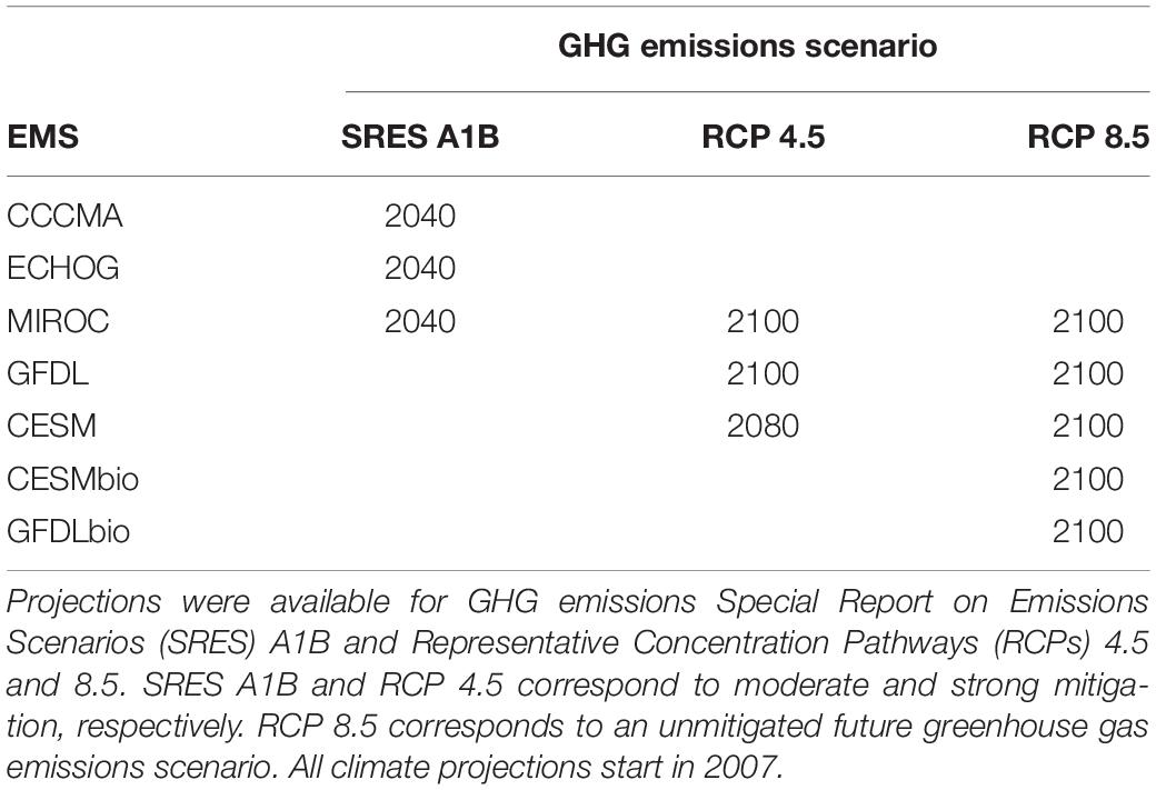
Table 1. Overview of the temporal extent of projections from Earth System Models (ESMs) that were used to generate ensemble predictions of the eastern Bering Sea food web.

The second set of ESMs included: MIROC, the Community Earth System Model (CESM), and the Geophysical Fluid Dynamic Laboratory ESM2M model (GFDL-ESM2M, herein simply GFDL; Table 1). These ESMs were archived by CMIP5 and span CMIP5 member variability (Taylor et al., 2012). Under this set of ESMs, downscaling of projections were performed through 2100 when possible for IPCC Representative Concentration Pathways (RCPs) 4.5 and 8.5, which correspond to futures with moderate and “business as usual” GHG emissions, respectively (Hermann et al., 2019; Table 1). ESMs in both sets were originally selected based on performance for the Bering Sea under present conditions and the availability of physical and biogeochemical output (Hermann et al., 2016, 2019).

ESM projections were dynamically downscaled using a biophysical model for the EBS (Hermann et al., 2019). Briefly, daily atmospheric and monthly oceanic outputs from the ESMs were interpolated in space and time for use in the surface forcing and boundary conditions for the regional model (Hermann et al., 2013). The model was implemented at ∼10 km spatial resolution with ten vertical layers and spans the entire Bering Sea (Hermann et al., 2013). The biological component of the model consists of a Nutrient-Phytoplankton-Zooplankton model (NPZ) developed by Gibson and Spitz (2011) with modifications by Hermann et al. (2016). Biological groups in the biophysical model include small phytoplankton, large phytoplankton, microzooplankton, small copepods, large copepods, krill (euphausiids), jellyfish, and slow and fast sinking detritus, benthic detritus, and benthic infauna. In addition to the ESM projections, a hindcast simulation for the EBS was generated for year 1970–2015 using historical reanalysis atmospheric forcing and ocean lateral boundary conditions (Hermann et al., 2016).

C: Multispecies Size Spectrum Model

The MSSM is based on source code for the R package “mizer” (Scott et al., 2014), as modified by Reum et al. (2019) and with additional updates (Supplementary Appendix I). The MSSM captures predator-prey interactions between fish and crab species and includes a submodel to represent the catch allocation process for EBS fisheries. In total, the model includes nine fish species, three crab species, and three fish functional groups (Supplementary Table 1). The included species support economically significant fisheries or are important prey items for other predators in the EBS, and combined, accounted for ∼95% of the community biomass based on estimates from annual bottom trawl surveys. The species are able to feed on each other, as well as two background spectra that represent additional pelagic and benthic prey resources. Predator species in the MSSMs are distinguished by several traits including maturation and maximum sizes, feeding and growth rates, and preferences for prey species and sizes (Supplementary Table 1). Additional details of the core model structure and prey selection parameterizations are available in Reum et al. (2019).

The submodel describing catch allocation in the EBS was incorporated into the MSSM to represent fishery management scenarios (Supplementary Appendix I). The aggregate total allowable catch (TAC) for several finfish and a few invertebrate fisheries is capped at 2 million metric tons for the larger Bering Sea-Aleutian Islands fisheries management zone (Livingston et al., 2011). Given this constraint, the North Pacific Fishery Management Council (a regional body that provides management recommendations for fisheries within the United States Economic Exclusive Zone surrounding Alaska) sets TACs by species based on stock assessment estimates of acceptable biological catch (ABC) and consideration of other factors such as market capacity, bycatch constraints, and fleet interests. A model describing TAC allocation for EBS fisheries, and that specifically used historical Council and fishery data to translate ABC to TAC and TAC to catches was adapted to generate catch predictions for each species depending on the fishery scenario (Supplementary Appendix I). ABCs were calculated for each species, based on current sloped harvest control rules that are intended to provide conservative catch recommendations, and the submodel returned realized catches that were used to calculate fishing mortality rates and total mortality calculations. The fishery submodel and ABC calculations are described further in Supplementary Appendix I.

At the MSSM level we sought to incorporate uncertainty into ensemble projections related to assumptions regarding temperature-dependencies on biological rates and, specifically, to evaluate the individual and interactive effects of temperature-dependencies on rates that influence body growth and intrinsic natural mortality. To do so, four MSSM variants were developed (Figure 1). The “baseline” model (M1) lacked temperature effects altogether, but background pelagic and benthic spectra were forced using downscaled projections from the biophysical model (Figure 1). The remaining models shared the same structure and forcings as M1, but differed in regard to whether temperature-dependencies were applied to the two categories of rates. The body growth category included maximum consumption, prey encounter, and metabolism rates and the intrinsic natural mortality category consisted solely of the intrinsic natural mortality rate which represents all mortality not explicitly captured by predation or fisheries in the model (Andersen et al., 2016). In mizer, intrinsic natural mortality is constant across body mass classes within species and calculated as an allometric function of species maximum body size (Scott et al., 2014) such that smaller species experience higher intrinsic natural mortality rates relative to larger species (Hartvig et al., 2011). The three additional MSSM variants (Figure 1) included temperature-dependencies in body growth-related rates (M2), intrinsic natural mortality rates (M3), and both body growth-related and intrinsic natural mortality rates (M4).

In models M2-4, Arrhenius temperature-dependent correction factors (Brown et al., 2004) were applied to biological rates. Originally intended for describing temperature effects on chemical reaction rates, the Arrhenius function is also appropriate for approximating temperature effects on metabolism and other biological rates at the individual, population, and community levels over environmentally plausible temperature ranges (Kooijman, 2000; Brown et al., 2004). For a given rate τ, the Arrhenius-corrected value at temperature T (in Kelvin) was obtained following Eq. (1):

where E is the activation energy of heterotrophic metabolism (0.63 eV), k is the Boltzmann constant, 8.62 × 10^–5eV K^–1, and T_ref is the reference temperature (Brown et al., 2004). Temperature forcing was based on downscaled depth-averaged temperature projections that were averaged spatially and within 3 month intervals starting in January, in accordance with the time step of the MSSM. A seasonal T_ref was therefore used and was obtained from averaging downscaled hindcast of depth-averaged temperatures over the model calibration period (1982–1991). All downscaled time series of temperature, benthos, and pelagic prey used in projections were bias-corrected relative to mean seasonal differences with the hindcast for the overlapping period 2002–2014 (Supplementary Figure 1). Details of the bias-correction calculation are presented in Supplementary Appendix I.

We calibrated the MSSM using a multistep process that included the estimation of parameters that scale species abundances and tuning of prey species preferences. The model was calibrated to time-averaged estimates of SSBs, catches, and diets from the 1980s (1982–1991; Supplementary Appendix I). Additional post-calibration modifications were made to the baseline natural (non-predation) mortality rates of several species to improve correspondence between projected SSBs and stock assessment estimates and ensure that predators exhibited levels of density-dependent recruitment that were commensurate with levels implied by time series of recruitment and SSB from stock assessments (Supplementary Appendix I). To validate the final calibrated models, all four variants of the MSSM were forced with historical fishing mortality rates (Fs) and hindcast time series of temperature and benthic and pelagic resource spectra from 1982 to 2014. Four validation criteria were evaluated: (1) correspondence of diet projections to data from outside the calibration time period (2005–2014); (2) correspondence between observed and predicted weight-at-age relationships; (3) overlap in the 95% confidence intervals for long-term linear trends between projected and observed SSBs; and (4) continued persistence of stocks when the models were projected forward assuming average historical climate conditions and status quo fisheries management from 2014 through 2100.

We focused on matches between long-term trends rather than simple correlation because population dynamics are partly controlled by stochastic recruitment events and these processes are not represented in the current class of MSSMs. This issue extends to other types of marine food web models where emphasis in model tuning has commonly been placed on matching averages and trends (e.g. Kaplan and Marshall, 2016). The last criteria was based on the observation that no finfish stocks have been overfished in the EBS and that the healthy status of EBS stocks is attributable in part to current (status quo) management practices (Livingston et al., 2011). We provide a thorough overview of the calibration and validation procedure in Supplementary Appendix I. The final post-calibrated MSSMs (all four variants) met the validation criteria and produced long-term trends that were similar to those from stock assessments (Supplementary Appendix I).

Fishery Management Scenarios

We evaluated three fishery management scenarios based on current policies for setting total allowable catch (TAC). This procedure is essential because the Bering Sea-Aleutian Islands ecosystem cap requires that individual species TACs be reduced so that the sum of all species is at or below the 2 million metric ton ecosystem cap (Hollowed et al., 2019). We considered scenarios in which: (1) TAC was allocated based on recent historical patterns (“status quo”); (2) pollock and Pacific cod TAC is increased up to 10% relative to status quo at the cost of lower flatfish TAC, and (3) flatfish TAC was increased up to 10% relative to status quo at the cost of lower pollock and Pacific cod TAC. For brevity, we herein refer to the scenarios as the “status quo,” “gadid,” and “flatfish” scenarios, respectively. The gadid and flatfish scenarios have been developed through examinations of historical fishing data and extensive conversations with members of the North Pacific Fishery Management Council and other stakeholders about the key decisions in the TAC-setting process. The scenarios represent realistic shifts in management and harvest behavior along what managers have identified as a key axis of decision-making. The shift could be motivated by combinations of economic factors, more stringent bycatch limits in different fisheries, or technological improvements that reduce the cost of bycatch avoidance.

Ensemble Projections

In total, seven ESMs were included in the model ensemble, and projections of these models under multiple GHG emissions scenarios were obtained, resulting in 11 unique ESM and GHG emission scenario projections that were downscaled to the EBS (Table 1). In turn, each unique downscaled projection was used to force M1-4 under the three catch allocation scenarios, resulting in 11 ⋅ 4 ⋅ 3 = 132 ensemble projections. All simulations were initiated in 1982 and forced with historical fishing mortality rates through 2014 (e.g. Blanchard et al., 2014) and thereafter downscaled bias-corrected projections of plankton and benthos prey (M1-4) and depth-averaged temperatures (M2-4). Catches and fishing mortality rates after 2014 were obtained from the catch allocation submodel.

Partitioning Uncertainty

We partitioned uncertainty (variance) in the ensemble projections into five distinct factors that were categorized as scenario (GHG and fishery management) and structural (ESM and MSSM) uncertainty and internal variability. Internal variability in climate projections on annual to decadal time scales includes phenomena such as the El Nino Southern Oscillation (ENSO), Pacific Decadal Oscillation (PDO), or North Atlantic Oscillation (NAO). In addition, internal variability can emerge within biological systems at similar time scales due to predator-prey cycles or other density-dependent growth, recruitment or mortality processes (Cheung et al., 2016). Internal variability is emergent in many types of complex systems, and outcomes are typically sensitive to initial starting conditions. If multiple realizations based on different starting conditions are available, the variance component associated with internal variability at a given time slice can be estimated along with other uncertainty sources using Analysis of Variance (ANOVA) models (e.g. Yip et al., 2011; Bosshard et al., 2013). However, similar to other climate and ecosystem simulation studies (e.g. Hawkins and Sutton, 2009; Gårdmark et al., 2013), our ensemble projections lacked multiple realizations that differ in initial conditions only. Instead, we used an alternative approach based on Hawkins and Sutton (2009) and Cheung et al. (2016).

First, the raw projection outputs y for each ESM m, MSSM variant v, GHG scenario g, fishing scenario f, and year t are written as:

where a reference level (invariant in time) for each unique ensemble member is denoted by μ_ref, the long-term trend with y is represented by a smooth spline function z, and the regression residual error (due to internal variability) is ε. For each ensemble realization, the reference level is the 1995–2014 mean state. The variance of y (V_y) is described as a function of time t following Eq. (3):

The estimate of internal variability is the variance (V_ε) of the residual regression error ε(m,v,r,f,t):

and is considered to have constant variance over time. In their original formulation, Hawkins and Sutton (2009) assumed V_ε was constant across the complete projection time span. We instead calculate a V_ε for each of three time blocks (2015–2040, 2041–2080, and 2081–2100) to account for changes in the representation of different ESMs and GHG scenarios in the ensemble projections (Table 1).

V_z, the variance associated with z(m,v,g,f,t), is calculated as:

where $z(\cdot ,\cdot ,\cdot ,\cdot ,t)$ is the overall mean at time-step t of the smooth spline trends; therefore, it measures the spread of ensemble simulations trends around the ensemble mean trend.

We used commonality analysis (Whittaker, 1984; Ray-Mukherjee et al., 2014) to decompose V_z into components that were uniquely and jointly associated with the four structural and scenario factors at time-step t. The approach entails performing multiple regression on the response variable (z), estimating the proportion of variance “explained” (R²) by the four factors, and decomposing R² into unique and shared components (Ray-Mukherjee et al., 2014). The method proceeds as follows. For factor x₁, the proportion of variance uniquely explained by x₁ is obtained by first regressing z on the full set of factors (x₁, x₂, x₃, and x₄) and the proportion of variance explained by the model ($R_{1,2,3,4}^2$) is calculated. Note, only main effects are included in the regression model. A second regression model is then applied, but excluding x₁. The proportion of variance uniquely explained by x₁ ($R_{1|2,3,4}^2$) is obtained by subtracting $R_{2,3,4}^2$ from $R_{1,2,3,4}^2$. Variance jointly explained by x₁ and the remaining factors is found by regressing z on x₁, obtaining the corresponding explained variance ($R_1^2$), and subtracting $R_{1|2,3,4}^2$ from $R_1^2$.

The absence of replicates (multiple realizations based on different initial conditions) meant that a fully saturated regression model with second, third and fourth order interaction terms would have zero degrees of freedom and no residual error. Consequently, we ascribed the “unexplained variance” associated with a model consisting only of main effect terms (that is, 1 – $R_{1,2,3,4}^2$) to variance associated with higher order interactions. We calculated the total variance associated with interaction terms for comparative purposes, but did not decompose it further since these components can be minor relative to those associated with the main effects and difficult to reliably estimate when replication at the lowest levels is limited (e.g. Yip et al., 2011).

We partitioned uncertainty in projections of catch, SSB, and mean weight for the community in aggregate and for individual species. We grouped species according to similarities in the decomposition of their catch, SSB, and mean weight projection uncertainties over time using a hierarchical cluster analysis which was based on a Euclidean distance matrix of the partitioned uncertainties and using Ward’s minimum variance criteria. For a given species, year, and variable, the partitioned uncertainties were expressed as proportions of the total uncertainty.

Interactions Between Fishery Management and GHG Mitigation Scenarios

We evaluated 2090 (mean for years 2081–2100) ensemble projections of abundance size spectra and catches, SSBs, and mean body weights to identify (1) differences between fishing scenarios in a warmer future (RCP 8.5) and (2) potential improvement in outcomes if GHG mitigation (RCP 4.5) is pursued. Specifically, we calculated average changes in 2090 projections relative to historical (1995–2014) levels for each fishing scenario under RCP 8.5. The effect of GHG mitigation was calculated as the difference in 2090 outcomes under scenario RCP 4.5 from those under RCP 8.5.

We characterized the reliability of ensemble projections in terms of the level of agreement in projecting positive or negative changes in relative values (e.g. Meehl et al., 2007; Bopp et al., 2013; Bryndum-Buchholz et al., 2019). Percent sign agreement (SA) was calculated as:

where P and N are the total number of positive and negative projections, respectively, and n is the total number of projections in the ensemble. If 50% of the ensemble projections are positive and 50% are negative the resulting SA is zero because every positive projection is matched by an opposing negative projection and vice versa. We focused on SA to emphasize qualitative differences in long-term ensemble projections. We considered SA of projections “high” and “low” when values were ≥80 and <80%, respectively.

Temperature Effects

We compared 2090 projections of relative change in abundance size spectra, catches, SSB, and mean body size under the different temperature models (M1-4). To simplify comparisons, the calculation was limited to projections made under the status quo fishing scenario and RCP 8.5 which included the largest changes in temperature. The ensemble mean and SA were calculated for each model output.

In addition, we calculated the cumulative effects of the temperature-dependency assumptions. Previous studies of cumulative ecological impacts have proposed methods for classifying interactions between stressors as synergistic, additive, or antagonistic (e.g. Crain et al., 2008; Griffith et al., 2011). However, if the individual effects of two “treatments” have opposing signs, assigning the interaction of the two treatments into these categories is not straightforward (Kaplan et al., 2013). Instead, we calculated whether the sum of the individual effects of temperature assumptions represented in M2 and M3 were above, below or similar to outcomes predicted under the combined model, M4 (Kaplan et al., 2013). The deviation (d₁,₂) of the interaction from the value expected if the individual effects were additive was obtained following (Kaplan et al., 2013):

where Y_AB is the ensemble mean value (catch, SSB, or mean weight) predicted under M4 (the subscript AB denotes both “treatments” are included), Y_CT is the ensemble mean value predicted under M1 (the “control”), and Y_A and Y_B are the ensemble mean values under M2 and M3. All Y values are expressed as a percentage of the control value (Y_CT is always 100%). We considered values of d_1,2 from −5 to 5% as additive, and values below and above the range non-additive negative and non-additive positive, respectively (Kaplan et al. (2013).

Results

Community Ensemble Projections and Uncertainty

Projected changes in aggregate community catch, SSB, and mean body weight for the full ensemble trended negatively on average through the end of the century (see Figure 2A). Projected model outputs through 2060 spanned both positive and negative values but thereafter projected values were solely negative, that is, SA was 100% (Figure 2A; Table 2). Projection uncertainties for aggregate catch, SSB, and mean body mass were dominated by internal variability through ∼2040 (Figure 2A) but at longer time horizons (2040–2100) structural uncertainties (i.e. ESM and temperature-dependencies) dominated (Figure 2A). For catches, temperature-dependencies composed the largest uncertainty source whereas ESM was the greatest source of uncertainty for SSB and mean body weight (Figure 2A).

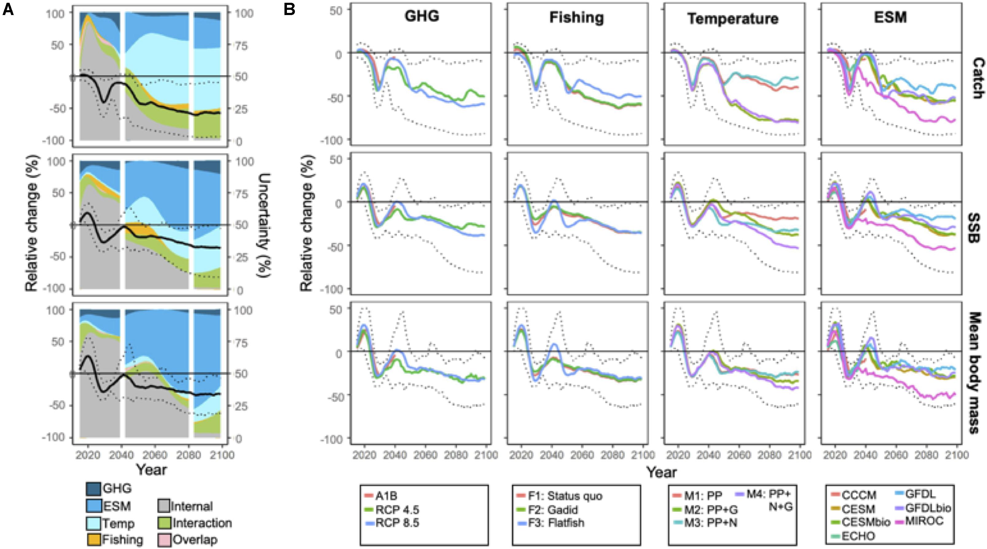
Figure 2. (A) Projections of total catches of EBS predator species, spawning stock biomass (SSB), and community mean body mass relative to 2014 levels. Black solid line corresponds to ensemble mean. Dotted lines indicate the minimum and maximum projections from the ensemble. Projection trends are overlaid on area plots that indicate the proportion of total variance in ensemble projections explained by scenario [greenhouse gas emissions (GHG) and fishing] and structural [Earth system model (ESM) and temperature effect] uncertainty and internal variability. The proportions explained by interactions between factors, and variance mutually explained by multiple factors (overlap) are also indicated. The vertical white lines demarcate time periods that differ with respect to the number of ESM members. For (B), solid colored lines correspond to projection averages within levels of the uncertainty source. For reference, maximum and minimum ensemble projections are noted (dotted lines).

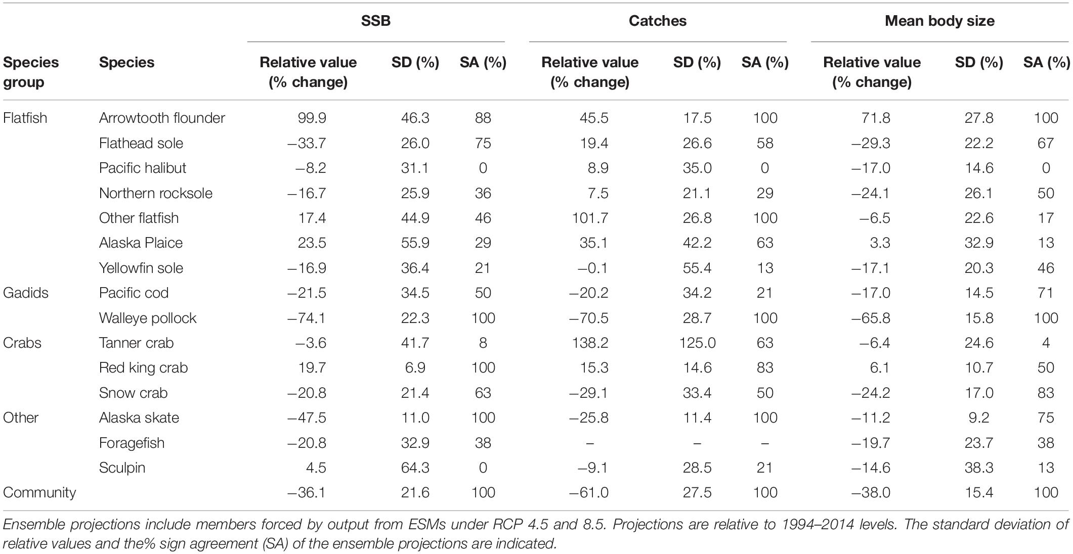
Table 2. Mean ensemble projections of average (2081–2100) relative SSB, catches and average body size for eastern Bering Sea food web members.

These general patterns were also evidenced by the larger spread of projected values when averaged according to ESM and MSSM variants as opposed to the GHG emission or fishery management scenario (Figure 2B). Future catches were substantially lower (∼30%) when body growth-related rates depended on temperature (M2 and M4 vs M1 and M3; Figure 2B). For SSB and mean body weight, the spread of projected values averaged according to ESMs were larger, and projected values under MIROC (the ESM with the warmest projections; Supplementary Figure 1) were considerably lower than under the remaining models (Figure 2B).

Although GHG scenarios accounted for only a small proportion of ensemble projection uncertainty over time (Figure 2A), average catches and SSB after 2060 were somewhat higher under mitigation scenario RCP 4.5 relative to the business-as-usual RCP 8.5 (Figure 2B). Among the fishery scenarios, total catches under the flatfish scenario were consistently higher than under the two alternatives after 2060, but differences for SSB and mean body weight among fishing scenarios were small (Figure 2B). In general, uncertainty due to interactions among the various sources of uncertainty increased over time and was larger in magnitude to the proportion directly associated with scenario uncertainty by the end of the century (both GHG and fishery; Figure 2A). Uncertainty explained by multiple sources (overlap) was minor (<1%, Figure 2B) for all variables.

Species Ensemble Projections and Uncertainty

Average full ensemble projections of relative change in SSB, catches, and mean body sizes for 2090 were negative for 66, 33, and 86% of species, respectively (Table 2), and for the majority of species, projections were more uncertain (as measured by SDs) than those for the aggregate community (Table 2). Overall, SDs ranged from 7 to 138% among model outputs (Table 2). Across model outputs, SA for projections were high for only four to five species and only pollock, the species with the largest biomass, had an SA value of 100% for all three model outputs (Table 2).

Species clustered into three groups based on similarity in the decomposition of projection uncertainty (Figure 3A). For the first group (yellowfin sole, Alaska plaice, other flatfish, and Alaska skate), internal variability and fishing scenario accounted for ∼10 to 50% of uncertainty in model outputs through 2040, but thereafter projection uncertainty was increasingly dominated by temperature assumptions (Figure 3B). Fishing scenario was the dominant source of uncertainty for catch projections in the second group (flathead sole and arrowtooth flounder) over time, but structural uncertainty sources (both ESMs and temperature assumptions) were important (>25%) after ∼2060 for SSB and mean body size (Figure 3B). For the third group, projection uncertainties were initially dominated by internal variability (∼50 to 75%), but after 2040, structural uncertainties became increasingly important (Figure 3B). For all groups and model outputs, uncertainty related to interactions between variables increased over time, and accounted for between ∼5 and 20% of uncertainty; GHG scenario uncertainty was a relatively minor contributor to uncertainty (<10%) for all groups and model outputs (Figure 3B).

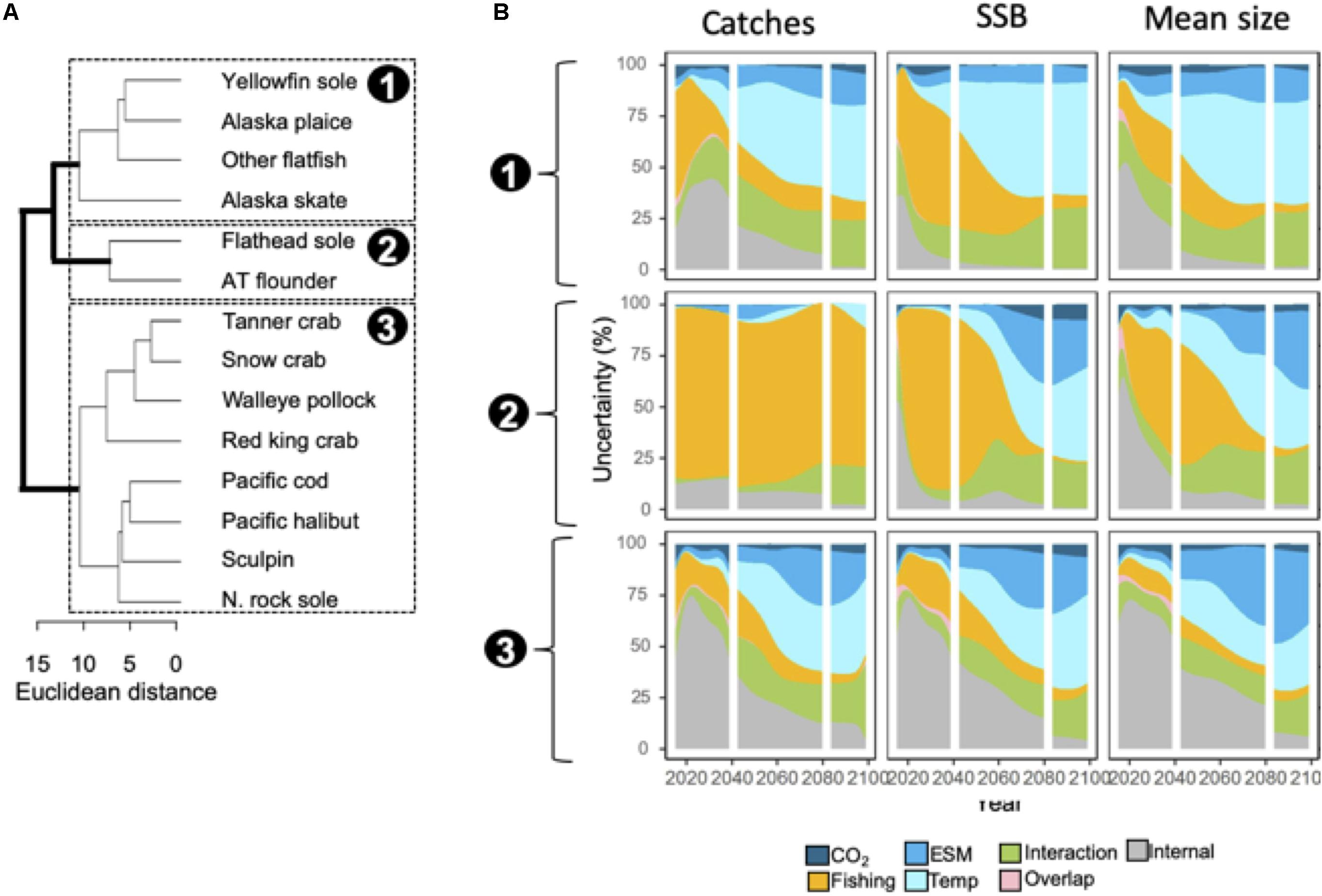
Figure 3. (A) Dendrogram of species similarity (Euclidean distance) based on relative importance of different uncertainty sources to catches, SSB, and mean weight ensemble projections. Three clusters were identified (labeled 1–3). (B) Area plots indicate the proportion of uncertainty associated with each source averaged across species within the three clusters. Species name abbreviations in panel (B): N. Northern; AT, arrowtooth.

Fishery Management and GHG Emissions

Overall, the largest differences in 2090 projections across fishery management scenarios included catches for flatfishes (flathead sole, other flatfish), which were ∼25 to 50% higher under the flatfish (F3) relative to status quo (F1) and gadid scenarios (F2) (Figure 4A). Reductions in total community catch were also ∼25% less severe under F3 relative to F1 and F3 (Figure 4A). For the remaining species, differences between model scenarios were smaller (Figure 4A).

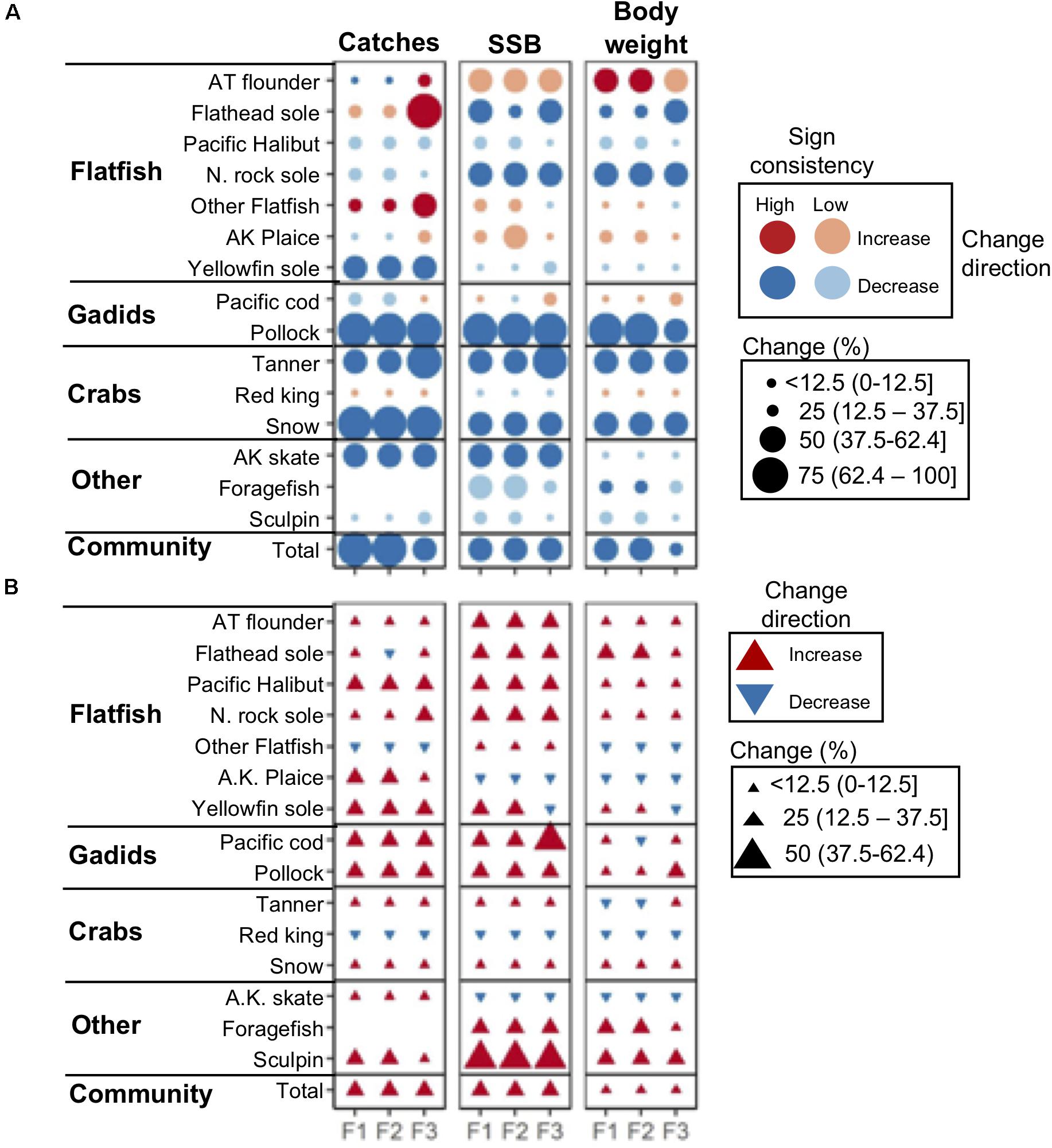
Figure 4. (A) Projected percent change in catches, SSB, and body weight by 2090 (mean 2080–2100) relative to historical (mean 1995–2014) levels assuming a “business-as-usual” GHG emissions scenario (RCP 8.5) and three scenarios of TAC setting preferences by fisheries management: status quo (F1), gadid (F2), and flatfish (F3). Dark and light symbol colors denote ensemble projections with high (≥80%) and low (<80%) sign agreement, respectively. (B) Percent difference between 2090 ensemble projections under GHG mitigation scenario RCP 4.5 and RCP 8.5. Species names abbreviations: AT, arrowtooth; A.K., Alaska; N., Northern.

Across all fishing management scenarios, SSB reductions were projected for the aggregate community and for 11 of the 15 species (Figure 4A). Reductions of ∼25% or more were projected for 6 species (flathead sole, Northern rock sole, walleye pollock, tanner and snow crab, and Alaska skate) with high SA. Smaller reductions (less than ∼25%) with low SA were projected for other species (yellowfin sole, Pacific halibut, red king crab, foragefish, and sculpin; Figure 4A). Both increases and decreases were projected across fishery management scenarios for the remaining species, with the notable exception of arrowtooth flounder which was projected to increase ∼50% across all fishery management scenarios (Figure 4A). These general patterns were similar to those observed for mean body weight for most species (Figure 4A), and were reflected in relative changes in abundance size spectra (Figure 5A). For each fishing scenario, reductions in abundance were projected across most body masses except for the interval dominated by arrowtooth flounder (∼10^3.7–10^4.0 g; Figure 5A).

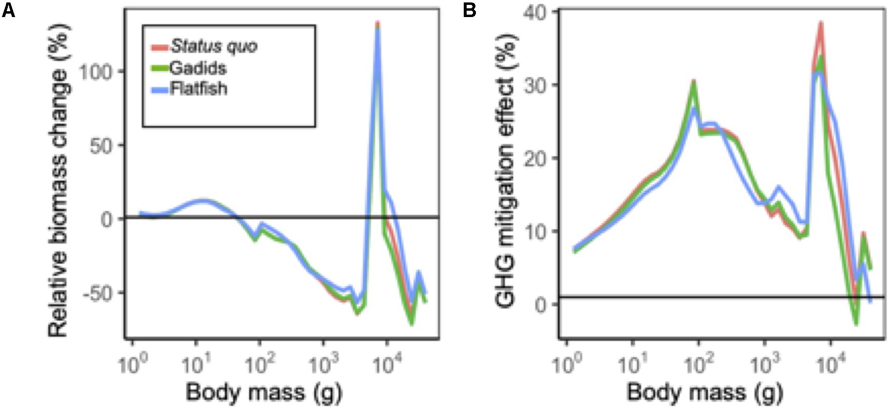
Figure 5. (A) Mean size spectra in 2090 (mean 2080–2100) relative to historical levels (mean 1995–2014) under each fishing scenario. All projections are under RCP 8.5. (B) Change in size spectra under GHG mitigation scenario RCP 4.5 relative to business as usual RCP 8.5 in 2090.

Under the GHG mitigation RCP 4.5 scenario, projections of SSB increased relative to RCP 8.5 across fishery scenarios for the aggregate community and 11 individual species (Figure 4B). The level of increase for individual species ranged up to ∼50% (sculpin) but for most species and model outputs, the increase was closer to ∼25%. Species that decreased in terms of SSB, included red king crab, Alaska plaice, and Alaska skate and reductions were <12.5% (Figure 4B). Overall, community abundance levels of individuals under RCP 4.5 increased ∼10 to 40% across size classes (Figure 5B). Patterns of net change in mean body weight and catches for most species were similar to those for SSB between scenarios (Figure 4B).

Temperature Sensitivity

At the community level, model outputs from MSSM variants that included temperature-dependencies on body growth (M2 and M4) were ∼25% lower than those that did not (Figure 6). This general pattern also extended to the abundance size spectra: in size classes >10² g reductions in abundance were consistently largest under M2 and M4 (Figure 7A). For individual species, model outputs under M4 (body growth and intrinsic natural mortality) where usually lower than those projected under M1 (status quo), but the difference in model outputs between M1 and M2 and M3 was variable across species (Figure 6). Roughly a third of species exhibited cumulative temperature effects that were additive, a third that were positive non-additive, and a third that were negative non-additive for each model output (Figure 6). A mixture of cumulative responses was also observed for the abundance size spectrum: positive responses were observed for body sizes near ∼10^1.8 and ∼10⁴ and negative responses dominated from between ∼10² and 10^3.8 g (Figure 7B).

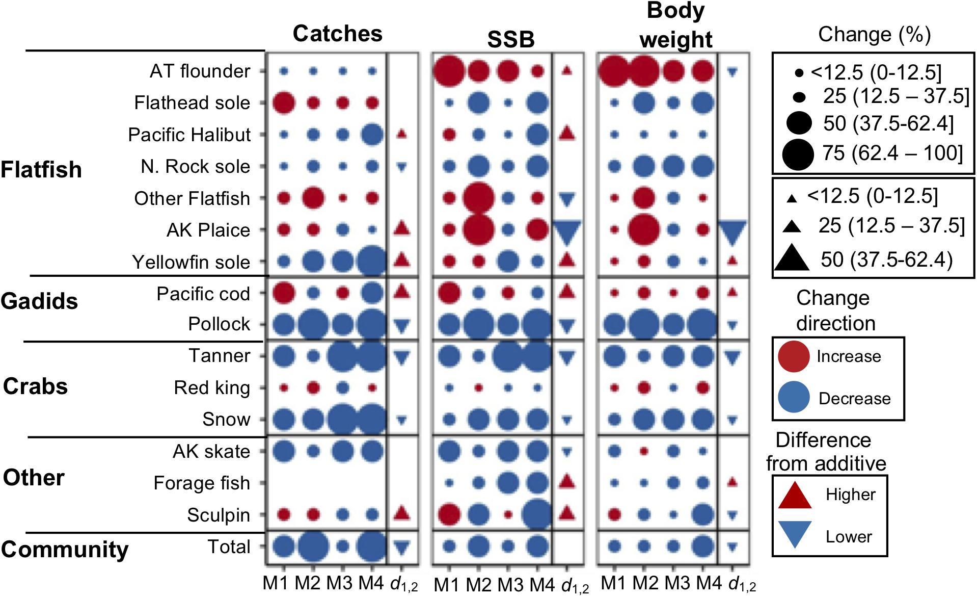
Figure 6. Mean projected changes in 2090 catches, SSB, and mean body size under RCP 8.5 and assuming status quo fishing for MSSM variants that assume the following temperature-dependencies on biological rates: none (M1), body growth-related rates (M2), intrinsic natural mortality (M3), and intrinsic natural mortality and body growth-related (M4). Changes are relative to historical average conditions (1995 to 2014). For each species and variable, the cumulative effects (d_1,2) of natural mortality and body growth-related temperature-dependencies are provided as the difference from outcomes derived from the assumption that cumulative effects are additive (triangle symbol).

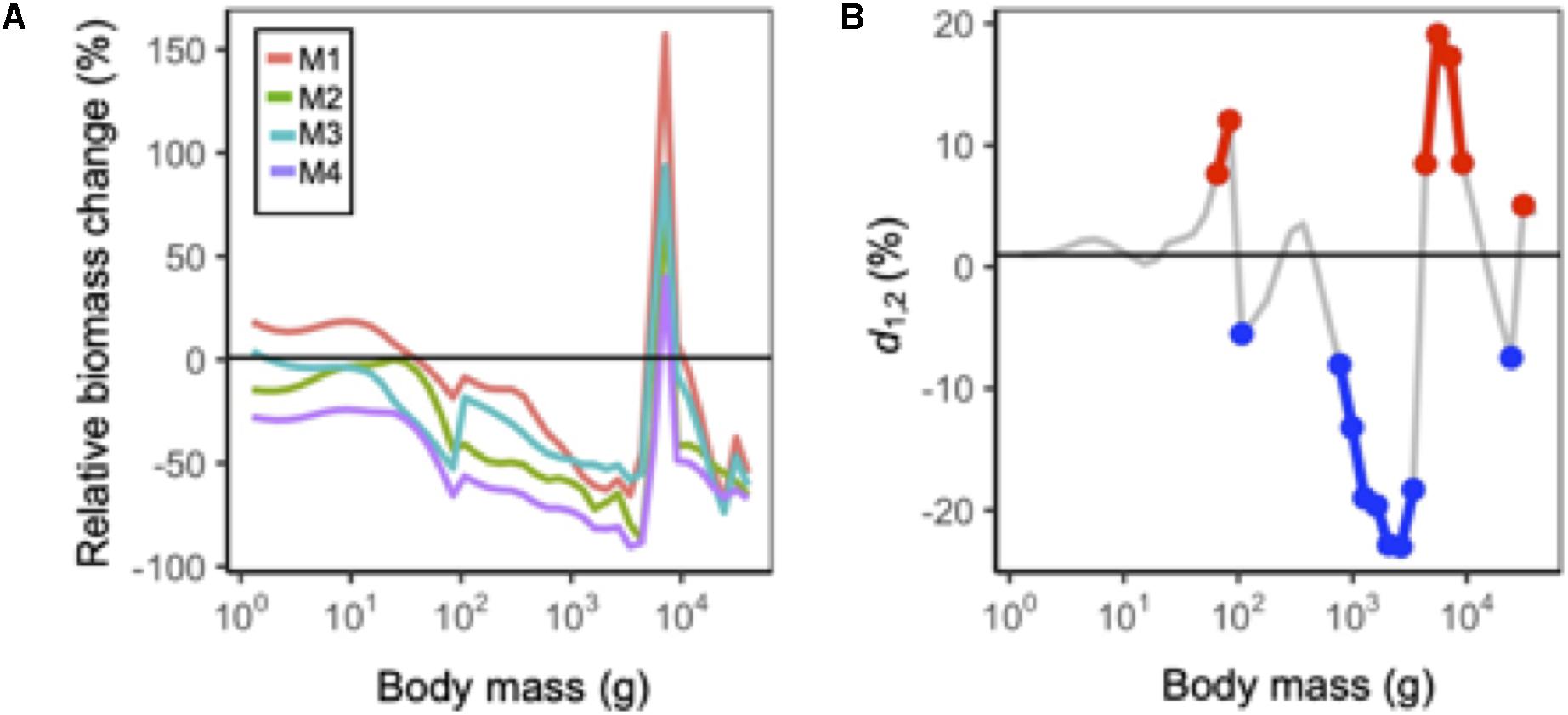
Figure 7. (A) Mean size spectra in 2090 relative to historical levels under each MSSM variant. All projections are under RCP 8.5 and assuming status quo fishing. (B) Difference in the cumulative effects of natural mortality and body growth-related temperature dependency assumptions from an additive effect (d₁,₂) on abundance at each size class. Red and blue points correspond to values larger and less than 5% of the additive effect, respectively.

Discussion

Our ensemble projections for the EBS food web lead to at least four significant insights. First, we show that aggregate community SSB, catches, and mean body weight (which are weighted toward pollock and which declines overtime), are likely to decrease by 2090 but ensemble projections for the majority of individual species were a mixture of increasing and decreasing trends. Second, structural uncertainty (both ESM and temperature-dependencies) dominated long-term (2060–2100) projections for many aggregate and species-level variables, which contrasts with global climate model ensemble projections of physical variables. In those studies, GHG emissions scenarios typically dominate end-of-century projection uncertainty (e.g. Hawkins and Sutton, 2009). Third, we show that temperature-dependencies on individual-level processes can impact emergent community- and species-level variables in complex and often non-additive ways. This highlights a critical aspect of structural uncertainty in climate-driven food web projections and the importance of frameworks such as MSSMs for scaling temperature-dependencies in individual-level processes to populations and communities. Last, while contributing less to long-term projection uncertainty, the moderate GHG mitigation scenario RCP4.5 also decreased the severity of projected long-term reductions in SSB, catches, and mean body weight for the majority of species relative to the business-as-usual emissions scenario across the different fisheries management scenarios. These outcomes demonstrate how policies and decision-making related to global GHG emissions may filter down to impact the trajectory of regional systems.

The results suggest future reductions in EBS benthic and pelagic prey resource spectra will decrease aggregate community biomass and fisheries yield. Overall, pollock composes ∼60% of the total fish biomass in the EBS and drove reductions in aggregate community biomass, catches, and mean body weight. Generally considered a forage species, pollock feed primarily on pelagic resource spectra prey and as they grow fish and benthic invertebrates comprise larger proportions of their diet. In downscaled projections, average pelagic and benthic resource spectrum prey densities decline ∼25% and 35% and 18 and 29% under RCP 4.5 and 8.5, respectively, by 2090. This largely caused the reductions in pollock productivity and aggregate community variables across fishery management scenarios. Interestingly, the negative trend is similar to projections from EBS pollock studies that estimated environmental stock-recruit relationships and forced recruitment with sea surface temperature projections using both single-species (Ianelli et al., 2011; Mueter et al., 2011) and age-structured multispecies models (Holsman et al., 2016; Ianelli et al., 2016; Spencer et al., 2016). The agreement in pollock trends across the different regional modeling studies is encouraging in terms of establishing confidence in projections, and contrasts with inconsistent total fish biomass projections from global-scale simulation studies (Cheung et al., 2010; Lefort et al., 2015; Lotze et al., 2018). That said, the directions of long-term trends in the ensemble were mixed for most other species and, with a few exceptions (e.g. Wilderbuer et al., 2002; Hollowed et al., 2009; Szuwalski and Punt, 2012), other regional projection studies are unavailable for these species. The ambiguity indicates heightened caution is warranted in drawing conclusions regarding the absolute value of potential net effects of climate change on the majority of EBS species using only the present model ensemble and that considerable room for improvement exists.

Our analysis of projection uncertainty provides descriptive summaries of key sources of variation, clustered species with similar sensitivities, and provides a basis for setting research priorities for refining ensemble projections (Evans et al., 2015; Cheung et al., 2016). Importantly, we show that structural uncertainties dominate intermediate- and long-term ensemble projections and, for the majority of species, ESMs were the largest uncertainty source. ESM climate projections are more variable for high latitude seas relative to other locations in part due to seasonal sea-ice cover dynamics that strongly impact other physical properties and the seasonal production cycle (Hawkins and Sutton, 2009). The number of ESMs used in the current study is small, but were selected to span CMIP5 member variability for EBS projections (Hermann et al., 2019). Decreasing this uncertainty source may be possible by applying more stringent EBS-specific validation criteria to further limit the ESM suite (Stock et al., 2011). Alternatively, including a larger set of IPCC-class ESMs in the ensemble could also help characterize the central tendency and spread of projections. Methods for expanding the number of ESMs in the ensemble, such as the development of statistical models to generate predictions of downscaled forcing variables based on relationships estimated from smaller subsets of dynamically downscaled ESMs, may prove valuable in this regard (e.g. Hermann et al., 2019).

The strong influence of temperature-dependencies on model outputs reinforces findings from sensitivity analyses performed on other size-based food web models (Maury et al., 2007) and highlights an important consideration when interpreting climate-driven projections from food web models forced with only primary production (e.g. Brown et al., 2010; Howell et al., 2013). At the community-level, temperature-dependencies on both categories of biological rates lowered catches, SSB, mean body weight, and abundance across size classes, but the level of decrease was highly variable across species and model outputs, in part because each species relies on different prey and is vulnerable to different predators. Consequently, the indirect effects of temperature that propagate through the food web may oppose or amplify direct temperature effects depending on the species and result in net outcomes that are difficult to anticipate. This complexity is exemplified in part by the mixture of additive, non-additive negative, and non-additive positive cumulative effects observed across body size intervals in the size spectrum and for individual species and model outputs. Ultimately, identifying how climate change impacts will manifest in ecological communities requires accounting for species interactions and our findings underscore the value of mechanistic models such as MSSMs for linking individual-level climate impacts to population and community-level outcomes.

Structural uncertainty related to temperature assumptions was also important for most long-term projections, but relative importance can also easily be change based on which models are represented in the ensemble. For instance, the baseline variant M1 represents an extreme endpoint and was included to bracket the range of model structures with regard to temperature and to evaluate potential non-additivity between different temperature-dependencies. Removing M1 from the ensemble would reduce projection uncertainty and could be justified based on the pervasive influence of temperature on biological rates (Brown et al., 2004). That said, in the absence of detailed species-specific information, the model set could also be expanded to represent other general but more nuanced hypotheses regarding temperature effects. For instance, the scaling of temperature-dependencies may change with ontogeny (Lindmark et al., 2018), differ across biological rates (Englund et al., 2011; Rall et al., 2012), or scale with temperature in a manner different from that described by the Arrhenius correction factor (Woodworth-Jefcoats et al., 2019). The latter may occur if species are currently at or near their thermal maximum. If so, additional warming could reduce rates ultimately controlling body growth, for example (Woodworth-Jefcoats et al., 2019). In the EBS, this issue may emerge for some species, particularly those with restricted northern distributions (e.g. snow crab, Northern rock sole) if the warmest future scenarios are realized. As our understanding of temperature effects on individuals and communities evolves, the ensemble members can be updated to formalize other possibilities, for instance, the effects of temperature-driven changes in phenology or distribution, and help identify the most consequential assumptions to projecting future system states.

Despite uncertainty in the absolute value of climate change impacts, we show that pursing GHG mitigation scenario RCP 4.5 ameliorated reductions in catches, SSB, mean body size, and abundance relative to business-as-usual RCP 8.5. These findings add to a growing body of research that demonstrate potential benefits to advancing coordinated, global-scale policies that abate GHG emission rates (Barange et al., 2014; e.g. Bryndum-Buchholz et al., 2019; Lotze et al., 2018). Importantly, we also show that these benefits were realized across the different fishery management scenarios for the majority of species over the long-term and that community-level catches were highest from after ∼2060 under the flatfish scenario relative to the other two scenarios. This latter observation suggests fisheries on currently underutilized species such as Arrowtooth flounder, flathead sole, Alaska plaice, and other flatfishes may partly offset future losses in pollock catches owing to climate change. Realization of the fishery management scenarios, however, is based on additional contingencies such as the opening of new markets and improvement in fishing gear technology and therefore suggests a direction in which to steer the larger EBS socioecological system.

The fishery management scenarios we considered are merely a subset of potential options and are premised on current fishery management polices remaining intact into the future. However, the framework can easily be adapted to evaluate a wider range of fishery management strategies including the effects of significant policy changes, for instance, modification or elimination of the 2 million m ton cap on TAC or the use of versions of multispecies maximum sustainable yield (Collie and Gislason, 2001; Moffitt et al., 2016) for setting ABCs rather than the currently used single-species version. To further increase the realism of different fishery management scenarios, methods for updating the reference SSBs that are used to calculate ABCs on annual or semi-annual time-scales would also be desirable to more closely simulate the management decision-making process. While room for improvement exists, the representation of the complex TAC setting process in the EBS is a major strength of our modeling framework because different fishery management strategies and scenarios can be compared to status quo management, and will be useful for exploring futures based on different regionalized socioeconomic pathways (Maury et al., 2017).

Due to computational demands, we were unable to evaluate several additional uncertainty sources. For instance, we did not address parametric uncertainty, but we note that uncertainty in parameters controlling allometric relationships and life history traits can strongly influence MSSM projections (Zhang et al., 2015). Outputs from the biophysical model, such as primary production, are also sensitive to biological parameterization uncertainty (Gibson and Spitz, 2011) and the issue also extends to ESMs. We did not incorporate parameter uncertainty because of practical computational constraints and because we sought to focus on uncertainty sources that have received less treatment in the ecological literature (Cheung et al., 2016). That said, methods for efficiently sampling parameter space to represent this uncertainty in the ensemble are available (e.g. Gibson and Spitz, 2011; Thorpe et al., 2015) and it is an important area for future research. Stochasticity in the stock-recruit relationships was also not represented in the MSSM. Consequently, the projections are based on the assumption that average recruitment relationships hold over time. Stochasticity in recruitment (or in parameters that directly control recruitment), can be a major uncertainty source in MSSM predictions (Blanchard et al., 2014; Zhang et al., 2016) and quantifying this uncertainty would help frame the importance of improving basic understanding of recruitment processes relative to other aspects of system structure. Last, we focused on two major climate forcings (shifts in basal prey resources, temperature), but other climate effects including ocean acidification, deoxygenation, or distributional shifts due to changes in habitat may also be important future drivers on fish and crab dynamics. As projections of additional variables become available for the EBS (e.g. Pilcher et al., 2018) and our understanding of their biological impacts improves, the model ensemble can be updated to consider a larger array of climate drivers.

Modeling frameworks that link global climate processes to regional ecological systems are vital test beds for evaluating management strategies under climate change (e.g. Weijerman et al., 2016; Hollowed et al., 2019). The framework presented here makes significant inroads in this regard and offers a template for other systems. Overall, we show that community-level catches, SSB, and mean body size are likely to decline for the EBS over the following century, but the level of decline is dominated by structural uncertainty. For many individual species, structural uncertainty also dominated projections, but for a subset (e.g. Arrowtooth flounder, flathead sole) fishery management scenario was instead important. This information can help inform and prioritize development of more concerted research programs based on both the species and objective. While we have partly focused on one facet of structural uncertainty at the MSSM level, we note that other single and multispecies models may also offer plausible representations of EBS fish and crab species dynamics and a major goal of ACLIM is to bracket the possible range of ecological effects of climate change by including models that differ in terms of their strengths and weaknesses (Hollowed et al., 2019). We expect ensemble projections that include a broader set of structurally distinct higher trophic level models will increase projection uncertainty. The estimates in the current study should therefore be viewed as conservative.

The method we propose for decomposing projection uncertainty can easily be adapted to account for additional categories of uncertainty represented in future ACLIM model suites and could be applied to other varieties of ensemble projections retroactively to glean further insight. Our modeling framework allows evaluation of different management and policy options and, like other ecosystem models, is best viewed as a strategic rather than tactical tool for supporting decision-making (e.g. Fulton et al., 2011; Andersen et al., 2016). In this vein, our efforts to characterize uncertainty in projections should facilitate uptake of results by resource managers and policy-makers alike (Addison et al., 2013; Cheung et al., 2016).

Data Availability Statement

The datasets generated for this study are available on request to the corresponding author.

Author Contributions

JR conceived of the study, developed the model code, performed the simulations and analysis, and drafted the manuscript. JB, KH, KA, and ABH helped conceive the study and aided with writing. AF and ACH provided code and text describing the eastern Bering Sea fishery system. WC and AJH provided downscaled climate projections for forcing the food web model. AP provided input on simulation design and analysis and contributed to writing.

Funding

This study was partially by the Alaska Climate Change Integrated Modeling project (ACLIM) and was supported by grants through the NOAA National Marine Fisheries Service Fisheries and the Environment (FATE) program, the Stock Assessment Analytical Methods (SAAM) program, the Climate Regimes & Ecosystem Productivity (CREP), the Economics and Human Dimensions Program, the NOAA Alaska Fisheries Science Center, the NOAA Integrated Ecosystem Assessment Program (IEA), and the NOAA Research Transition Acceleration Program (RTAP). This publication is partially funded by the Joint Institute for the Study of the Atmosphere and Ocean (JISAO) under NOAA Cooperative Agreement NA15OAR4320063, Contribution No. 2020-1053. We also acknowledge support from the Australian Research Council Discovery Project DP170104240 (“Rewiring Marine Foodwebs”).

Conflict of Interest

The authors declare that the research was conducted in the absence of any commercial or financial relationships that could be construed as a potential conflict of interest.

Acknowledgments

Valuable comments and suggestions were provided by P. Woodworth-Jefcoats, G. Whitehouse, and K. Murphy on earlier versions of the manuscript.

Supplementary Material

The Supplementary Material for this article can be found online at: https://www.frontiersin.org/articles/10.3389/fmars.2020.00124/full#supplementary-material

References

Addison, P. F., Rumpff, L., Bau, S. S., Carey, J. M., Chee, Y. E., Jarrad, F. C., et al. (2013). Practical solutions for making models indispensable in conservation decision-making. Diver. Distrib. 19, 490–502. doi: 10.1111/ddi.12054
Andersen, K. H., Jacobsen, N. S., and Farnsworth, K. D. (2016). The theoretical foundations for size spectrum models of fish communities. Can. J. Fish. Sci. 73, 575–588. doi: 10.1139/cjfas-2015-0230
Barange, M., Merino, G., Blanchard, J. L., Scholtens, J., Harle, J., Allison, E. H., et al. (2014). Impacts of climate change on marine ecosystem production in societies dependent on fisheries. Nat. Clim. Change 4, 211–216. doi: 10.1038/nclimate2119
Berliner, L. M., and Kim, Y. (2008). Bayesian design and analysis for superensemble-based climate forecasting. J. Clim. 21, 1891–1910. doi: 10.1175/2007jcli1619.1
Blanchard, J. L., Andersen, K. H., Scott, F., Hintzen, N. T., Piet, G., and Jennings, S. (2014). Evaluating targets and trade-offs among fisheries and conservation objectives using a multispecies size spectrum model. J. App. Ecol. 51, 612–622. doi: 10.1111/1365-2664.12238
Blanchard, J. L., Heneghan, R. F., Everett, J. D., Trebilco, R., and Richardson, A. J. (2017). From bacteria to whales: using functional size spectra to model marine ecosystems. Trends Ecol. Evol. 32, 174–186. doi: 10.1016/j.tree.2016.12.003
Blanchard, J. L., Jennings, S., Holmes, R., Harle, J., Merino, G., Allen, J. I., et al. (2012). Potential consequences of climate change for primary production and fish production in large marine ecosystems. Philos. Trans. R. Soc. B 367, 2979–2989. doi: 10.1098/rstb.2012.0231
Bopp, L., Resplandy, L., Orr, J. C., Doney, S. C., Dunne, J. P., Gehlen, M., et al. (2013). Multiple stressors of ocean ecosystems in the 21st century: projections with CMIP5 models. Biogeosciences 10, 6225–6245. doi: 10.5194/bg-10-6225-2013
Bosshard, T., Carambia, M., Goergen, K., Kotlarski, S., Krahe, P., Zappa, M., et al. (2013). Quantifying uncertainty sources in an ensemble of hydrological climate-impact projections. Water Resour. Res. 49, 1523–1536. doi: 10.1029/2011wr011533
Brown, C. J., Fulton, E. A., Hobday, A. J., Matear, R. J., Possingham, H. B., Bulman, C., et al. (2010). Effects of climate-driven primary production change on marine food webs: implications for fisheries and conservation. Glob. Change Biol. 16, 1194–1212. doi: 10.1111/j.1365-2486.2009.02046.x
Brown, J. H., Gillooly, J. F., Allen, A. P., Savage, V. M., and West, G. B. (2004). Toward a metabolic theory of ecology. Ecology 85, 1771–1789. doi: 10.1890/03-9000
Bryndum-Buchholz, A., Tittensor, D. P., Blanchard, J. L., Cheung, W. W., Coll, M., Galbraith, E. D., et al. (2019). Twenty-first-century climate change impacts on marine animal biomass and ecosystem structure across ocean basins. Glob. Change Biol. 25, 459–472. doi: 10.1111/gcb.14512
Cheung, W. W., Lam, V. W., Sarmiento, J. L., Kearney, K., Watson, R. E. G., Zeller, D., et al. (2010). Large-scale redistribution of maximum fisheries catch potential in the global ocean under climate change. Glob. Change Biol. 16, 24–35. doi: 10.1111/j.1365-2486.2009.01995.x
Cheung, W. W. L., Frölicher, T. L., Asch, R. G., Jones, M. C., Pinsky, M. L., Reygondeau, G., et al. (2016). Building confidence in projections of the responses of living marine resources to climate change. ICES J. Mar. Sci. 73, 1283–1296. doi: 10.1093/icesjms/fsv250
Collie, J. S., and Gislason, H. (2001). Biological reference points for fish stocks in a multispecies context. Can. J. Fish. Aquat. Sci. 58, 2167–2176. doi: 10.1139/f01-158
Crain, C. M., Kroeker, K., and Halpern, B. S. (2008). Interactive and cumulative effects of multiple human stressors in marine systems. Ecol. Lett. 11, 1304–1315. doi: 10.1111/j.1461-0248.2008.01253.x
Doney, S. C., Ruckelshaus, M., Duffy, J. E., Barry, J. P., Chan, F., English, C. A., et al. (2012). Climate change impacts on marine ecosystems. Mar. Sci. 4, 11–37.
Englund, G., Öhlund, G., Hein, C. L., and Diehl, S. (2011). Temperature dependence of the functional response. Ecol. Lett. 14, 914–921. doi: 10.1111/j.1461-0248.2011.01661.x
Evans, K., Brown, J. N., Sen Gupta, A. S., Nicol, S. J., Hoyle, S., Matear, R., et al. (2015). When 1+1 can be >2: uncertainties compound when simulating climate, fisheries and marine ecosystems. Deep Sea Res. Part II Top. Stud. Oceanogr. 113, 312–322. doi: 10.1016/j.dsr2.2014.04.006
Fulton, E. A., Link, J. S., Kaplan, I. C., Savina-Rolland, M., Johnson, P., Ainsworth, C., et al. (2011). Lessons in modelling and management of marine ecosystems: the Atlantis experience. Fish Fish. 12, 171–188. doi: 10.1111/j.1467-2979.2011.00412.x
Gårdmark, A., Lindegren, M., Neuenfeldt, S., Blenckner, T., Heikinheimo, O., Müller-Karulis, B., et al. (2013). Biological ensemble modeling to evaluate potential futures of living marine resources. Ecol. Appl. 23, 742–754. doi: 10.1890/12-0267.1
Gibson, G. A., and Spitz, Y. H. (2011). Impacts of biological parameterization, initial conditions, and environmental forcing on parameter sensitivity and uncertainty in a marine ecosystem model for the Bering Sea. J. Mar. Sci. 88, 214–231. doi: 10.1016/j.jmarsys.2011.04.008
Griffith, G. P., Fulton, E. A., and Richardson, A. J. (2011). Effects of fishing and acidification-related benthic mortality on the southeast Australian marine ecosystem. Glob. Change Biol. 17, 3058–3074. doi: 10.1111/j.1365-2486.2011.02453.x
Guiet, J., Poggiale, J.-C., and Maury, O. (2016). Modelling the community size-spectrum: recent developments and new directions. Ecol. Modell. 337, 4–14. doi: 10.1016/j.ecolmodel.2016.05.015
Hartvig, M., Andersen, K. H., and Beyer, J. E. (2011). Food web framework for size-structured populations. J. Theor. Biol. 272, 113–122. doi: 10.1016/j.jtbi.2010.12.006
Hawkins, E., and Sutton, R. (2009). The potential to narrow uncertainty in regional climate predictions. Bull. Am. Met. Soc. 90, 1095–1108. doi: 10.1175/2009bams2607.1
Hermann, A. J., Gibson, G. A., Bond, N. A., Curchitser, E. N., Hedstrom, K., Cheng, W., et al. (2013). A multivariate analysis of observed and modeled biophysical variability on the Bering Sea shelf: multidecadal hindcasts (1970–2009) and forecasts (2010–2040). Deep Sea Res. II 94, 121–139. doi: 10.1016/j.dsr2.2013.04.007
Hermann, A. J., Gibson, G. A., Bond, N. A., Curchitser, E. N., Hedstrom, K., Cheng, W., et al. (2016). Projected future biophysical states of the Bering Sea. Deep Sea Res. II. 134, 30–47. doi: 10.1016/j.dsr2.2015.11.001
Hermann, A. J., Gibson, G. A., Cheng, W., Ortiz, I., Aydin, K., Wang, M., et al. (2019). Projected biophysical conditions of the Bering Sea to 2100 under multiple emission scenarios. ICES J. Mar. Sci. 76, 1280–1304. doi: 10.1093/icesjms/fsz111
Hollowed, A. B., Bond, N. A., Wilderbuer, T. K., Stockhausen, W. T., A’Mar, Z. T., Beamish, R. J., et al. (2009). A framework for modelling fish and shellfish responses to future climate change. ICES J. Mar. Sci. 66, 1584–1594. doi: 10.1093/icesjms/fsp057
Hollowed, A. B., Holsman, K. K., Haynie, A. C., Hermann, A., Punt, A. E., Aydin, K., et al. (2019). Integrated modeling to evaluate climate change impacts on coupled social-ecological systems in Alaska. Front. Mar. Sci. 6:775. doi: 10.3389/fmars.2019.00775
Holsman, K. K., Ianelli, J., Aydin, K., Punt, A. E., and Moffitt, E. A. (2016). A comparison of fisheries biological reference points estimated from temperature-specific multi-species and single-species climate-enhanced stock assessment models. Deep Sea Res. Part II Top. Stud. Oceanogr. 134, 360–378. doi: 10.1016/j.dsr2.2015.08.001
Howell, E. A., Wabnitz, C. C. C., Dunne, J. P., and Polovina, J. J. (2013). Climate-induced primary productivity change and fishing impacts on the Central North Pacific ecosystem and Hawaii-based pelagic longline fishery. Clim. Change 119, 79–93. doi: 10.1007/s10584-012-0597-z
Ianelli, J. N., Hollowed, A. B., Haynie, A. C., Mueter, F. J., and Bond, N. A. (2011). Evaluating management strategies for eastern Bering Sea walleye pollock (Theragra chalcogramma) in a changing environment. ICES J. Mar. Sci. 68, 1297–1304. doi: 10.1093/icesjms/fsr010
Ianelli, J., Holsman, K. K., Punt, A. E., and Aydin, K. (2016). Multi-model inference for incorporating trophic and climate uncertainty into stock assessments. Deep Sea Res. Part II Top. Stud. Oceanogr. 34, 379–389. doi: 10.1016/j.dsr2.2015.04.002
Kaplan, I. C., Gray, I. A., and Levin, P. S. (2013). Cumulative impacts of fisheries in the California current. Fish Fish. 14, 515–527. doi: 10.1111/j.1467-2979.2012.00484.x
Kaplan, I. C., and Marshall, K. (2016). A guinea pig’s tale: learning to review end-to-end marine ecosystem models for management applications. ICES J. Mar. Sci. 73, 1715–1724. doi: 10.1093/icesjms/fsw047
Keil, G., Cummings, E., and de Magalhaes, J. P. (2015). Being cool: how body temperature influences ageing and longevity. Biogerontology 16, 383–397. doi: 10.1007/s10522-015-9571-2
Kerr, S. R., and Dickie, L. M. (2001). The Biomass Spectrum. New York, NY: Columbia University Press.
Kooijman, S. A. L. M. (2000). Dynamic Energy and Mass Budgets in Biological Systems. New York, NY: Cambridge University Press.
Lefort, S., Aumont, O., Bopp, L., Arsouze, T., Gehlen, M., and Maury, O. (2015). Spatial and body-size dependent response of marine pelagic communities to projected global climate change. Glob. Change Biol. 21, 154–164. doi: 10.1111/gcb.12679
Lindmark, M., Huss, M., Ohlberger, J., and Gårdmark, A. (2018). Temperature-dependent body size effects determine population responses to climate warming. Ecol. Lett. 21, 181–189. doi: 10.1111/ele.12880
Livingston, P., Aydin, K., Boldt, J. L., Hollowed, A. B., Napp, J. M., et al. (2011). “Alaska marine fisheries management: advances and linkages to ecosystem research,” in Ecosystem Based Management for Marine Fisheries: An Evolving Perspective, eds A. A. Belgrano and C. C. Fowler (Cambridge: Cambridge Univ. Press), 113–152. doi: 10.1017/cbo9780511973956.006
Lotze, H. K., Tittensor, D. P., Bryndum-Buchholz, A., Eddy, T. D., Cheung, W. W., Galbraith, E. D., et al. (2018). Ensemble projections of global ocean animal biomass with climate change. bioRxiv [Preprint]
MacKenzie, B. R., Meier, H. M., Lindegren, M., Neuenfeldt, S., Eero, M., Blenckner, T., et al. (2012). Impact of climate change on fish population dynamics in the Baltic Sea: a dynamical downscaling investigation. AMBIO 41, 626–636. doi: 10.1007/s13280-012-0325-y
Marshall, K. N., Kaplan, I. C., Hodgson, E. E., Hermann, A., Busch, D. S., McElhany, P., et al. (2017). Risks of ocean acidification in the California current food web and fisheries: ecosystem model projections. Glob. Change Biol. 23, 1525–1539. doi: 10.1111/gcb.13594
Maury, O., Campling, L., Arrizabalaga, H., Aumont, O., Bopp, L., Merino, G., et al. (2017). From shared socio-economic pathways (SSPs) to oceanic system pathways (OSPs): building policy-relevant scenarios for global oceanic ecosystems and fisheries. Glob. Environ. Change 45, 203–216. doi: 10.1016/j.gloenvcha.2017.06.007
Maury, O., and Poggiale, J.-C. (2013). From individuals to populations to communities: a dynamic energy budget model of marine ecosystem size-spectrum including life history diversity. J. Theor. Biol. 324, 52–71. doi: 10.1016/j.jtbi.2013.01.018
Maury, O., Shin, Y. J., Faugeras, B., Ari, T. B., and Marsac, F. (2007). Modeling environmental effects on the size-structured energy flow through marine ecosystems. Part 2: simulations. Prog. Oceanog. 74, 500–514. doi: 10.1016/j.pocean.2007.05.001
Meehl, G. A., Stocker, T. F., Collins, W. D., Friedlingstein, P., Gaye, A. T., Gregory, J. M., et al. (2007). “Climate change 2007: the physical science basis,” in Contribution of Working Group I to the Fourth Assessment Report of the Intergovernmental Panel on Climate Change, chap. Global Climate Projections, eds M.L. Parry, O.F. Canziani, J.P. Palutikof, P.J. van der Linden, and C.E. Hanson (Cambridge: Cambridge University Press), 747–846.
Meier, H. E. M., Andersson, H., Arheimer, B., Blenckner, T., Chubarenko, B., Donnelly, C., et al. (2012). Comparing reconstructed past variations and future projections of the Baltic Sea ecosystem—first results from multi-model ensemble simulations. Environ. Res. Lett. 7:034005. doi: 10.1088/1748-9326/7/3/034005
Moffitt, E. A., Punt, A. E., Holsman, K., Aydin, K. Y., Ianelli, J. N., and Ortiz, I. (2016). Moving towards ecosystem-based fisheries management: options for parameterizing multi-species biological reference points. Deep Sea Res. II 134, 350–359. doi: 10.1016/j.dsr2.2015.08.002
Mora, C., Wei, C.-L., Rollo, A., Amaro, T., Baco, A. R., Billett, D., et al. (2013). Biotic and human vulnerability to projected changes in ocean biogeochemistry over the 21st century. PLoS Biol. 11:e1001682. doi: 10.1371/journal.pbio.1001682
Mueter, F. J., Bond, N. A., Ianelli, J. N., and Hollowed, A. B. (2011). Expected declines in recruitment of walleye pollock (Theragra chalcogramma) in the eastern Bering Sea under future climate change. ICES J. Mar. Sci. 68, 1284–1296. doi: 10.1093/icesjms/fsr022
Munch, S. B., and Salinas, S. (2009). Latitudinal variation in lifespan within species is explained by the metabolic theory of ecology. Proc. Nat. Acad. Sci. U.S.A. 106, 13860–13864. doi: 10.1073/pnas.0900300106
Murphy, J. M., Sexton, D. M., Barnett, D. N., and Jones, G. S. (2004). Quantification of modelling uncertainties in a large ensemble of climate change simulations. Nature 430:768. doi: 10.1038/nature02771
Niiranen, S., Yletyinen, J., Tomczak, M. T., Blenckner, T., Hjerne, O., MacKenzie, B. R., et al. (2013). Combined effects of global climate change and regional ecosystem drivers on an exploited marine food web. Global Change Biol. 19, 3327–3342.
Payne, M. R., Barange, M., Cheung, W. W., MacKenzie, B. R., Batchelder, H. P., Cormon, X., et al. (2015). Uncertainties in projecting climate-change impacts in marine ecosystems. ICES J. Mar. Sci. 73, 1272–1282.
Pecl, G. T., Araújo, M. B., Bell, J. D., Blanchard, J., Bonebrake, T. C., Chen, I.-C., et al. (2017). Biodiversity redistribution under climate change: impacts on ecosystems and human well-being. Science 355:eaai9214.
Persson, L., Van Leeuwen, A., and De Roos, A. M. (2014). The ecological foundation for ecosystem-based management of fisheries: mechanistic linkages between individual-, population-, and community-level dynamics. ICES J. Mar. Sci. 71, 2268–2280. doi: 10.1093/icesjms/fst231
Pilcher, D., Naiman, D., Cross, J., Hermann, A., Siedlecki, S., Gibson, G., et al. (2018). Modeled effect of coastal biogeochemical processes, climate variability, and ocean acidification on aragonite saturation state in the Bering Sea. Front. Mar. Sci. 5:508. doi: 10.3389/fmars.2018.00508
Rall, B. C., Brose, U., Hartvig, M., Kalinkat, G., Schwarzmüller, F., Vucic-Pestic, O., et al. (2012). Universal temperature and body-mass scaling of feeding rates. Philos. Trans. R. Soc. B 367, 2923–2934. doi: 10.1098/rstb.2012.0242
Ray-Mukherjee, J., Nimon, K., Mukherjee, S., Morris, D. W., Slotow, R., and Hamer, M. (2014). Using commonality analysis in multiple regressions: a tool to decompose regression effects in the face of multicollinearity. Method Ecol. Evol. 5, 320–328. doi: 10.1111/2041-210x.12166
Reum, J. C. P., Blanchard, J. L., Holsman, K. K., Aydin, K., and Punt, A. E. (2019). Species-specific ontogenetic diet shifts attenuate trophic cascades and lengthen food chains in an exploited ecosystem. Oikos 128, 1051–1064. doi: 10.1111/oik.05630
Scott, F., Blanchard, J. L., and Andersen, K. H. (2014). mizer: an R package for multispecies, trait-based and community size spectrum ecological modelling. Methods Ecol. Evol. 5, 1121–1125. doi: 10.1111/2041-210X.12256
Spencer, P. D., Holsman, K. K., Zador, S., Bond, N. A., Mueter, F. J., Hollowed, A. B., et al. (2016). Modelling spatially dependent predation mortality of eastern Bering Sea walleye pollock, and its implications for stock dynamics under future climate scenarios. ICES J. Mar. Sci. 73, 1330–1342. doi: 10.1093/icesjms/fsw040
Stabeno, P. J., Bond, N. A., Kachel, N. B., Salo, S. A., and Schumacher, J. D. (2001). On the temporal variability of the physical environment over the south-eastern Bering Sea. Fish. Oceanog. 10, 81–98. doi: 10.1046/j.1365-2419.2001.00157.x
Stock, C. A., Alexander, M. A., Bond, N. A., Brander, K. M., Cheung, W. W., Curchitser, E. N., et al. (2011). On the use of IPCC-class models to assess the impact of climate on living marine resources. Prog. Oceanog. 88, 1–27. doi: 10.1016/j.pocean.2010.09.001
Szuwalski, C. S., and Punt, A. E. (2012). Fisheries management for regime-based ecosystems: a management strategy evaluation for the snow crab fishery in the eastern Bering Sea. ICES J. Mar. Sci. 70, 955–967. doi: 10.1093/icesjms/fss182
Taylor, K. E., Stouffer, R. J., and Meehl, G. A. (2012). An overview of CMIP5 and the experiment design. Bull. Am. Met. Soc. 93, 485–498. doi: 10.1175/bams-d-11-00094.1
Tebaldi, C., and Knutti, R. (2007). The use of the multi-model ensemble in probabilistic climate projections. Philos. Trans. R. Soc. A 365, 2053–2075. doi: 10.1098/rsta.2007.2076
Thorpe, R. B., Le Quesne, W. J., Luxford, F., Collie, J. S., and Jennings, S. (2015). Evaluation and management implications of uncertainty in a multispecies size-structured model of population and community responses to fishing. Method Ecol. Evol. 6, 49–58. doi: 10.1111/2041-210x.12292
Weijerman, M., Fulton, E. A., and Brainard, R. E. (2016). Management strategy evaluation applied to coral reef ecosystems in support of ecosystem-based management. PLoS ONE 11:e0152577. doi: 10.1371/journal.pone.0152577
Whittaker, J. (1984). Model interpretation from the additive elements of the likelihood function. J. R. Stat. Soc. C 33, 52–64.
Wilderbuer, T. K., Hollowed, A. B., Ingraham, W. J. Jr., Spencer, P. D., Conners, M. E., Bond, N. A., et al. (2002). Flatfish recruitment response to decadal climatic variability and ocean conditions in the eastern Bering Sea. Prog. Oceanog. 55, 235–247. doi: 10.1016/s0079-6611(02)00081-2
Woodworth-Jefcoats, P. A., Blanchard, J. L., and Drazen, J. C. (2019). Relative impacts of simultaneous stressors on a pelagic marine ecosystem. Front. Mar. Sci. 6:383. doi: 10.3389/fmars.2019.00383
Woodworth-Jefcoats, P. A., Polovina, J. J., Dunne, J. P., and Blanchard, J. L. (2013). Ecosystem size structure response to 21st century climate projection: large fish abundance decreases in the central North Pacific and increases in the California Current. Glob. Change Biol. 19, 724–733. doi: 10.1111/gcb.12076
Yip, S., Ferro, C. A., Stephenson, D. B., and Hawkins, E. (2011). A simple, coherent framework for partitioning uncertainty in climate predictions. J. Clim. 24, 4634–4643. doi: 10.1175/2011jcli4085.1
Zhang, C., Chen, Y., and Ren, Y. (2015). Assessing uncertainty of a multispecies size-spectrum model resulting from process and observation errors. ICES J. Mar. Sci. 72, 2223–2233. doi: 10.1093/icesjms/fsv086
Keywords: uncertainty partitioning, predictive ecology, Arrhenius factor, body size, size-based food web, cumulative effects, commonality analysis
Citation: Reum JCP, Blanchard JL, Holsman KK, Aydin K, Hollowed AB, Hermann AJ, Cheng W, Faig A, Haynie AC and Punt AE (2020) Ensemble Projections of Future Climate Change Impacts on the Eastern Bering Sea Food Web Using a Multispecies Size Spectrum Model. Front. Mar. Sci. 7:124. doi: 10.3389/fmars.2020.00124
Received: 19 August 2019; Accepted: 17 February 2020;
Published: 17 March 2020.
Edited by:
Erik Olsen, Norwegian Institute of Marine Research (IMR), NorwayReviewed by:
Martina Hanneliese Stiasny, Norwegian Institute of Marine Research (IMR), NorwayMorgane Travers-Trolet, Institut Français de Recherche pour l’Exploitation de la Mer (IFREMER), France
Copyright © 2020 Reum, Blanchard, Holsman, Aydin, Hollowed, Hermann, Cheng, Faig, Haynie and Punt. This is an open-access article distributed under the terms of the Creative Commons Attribution License (CC BY). The use, distribution or reproduction in other forums is permitted, provided the original author(s) and the copyright owner(s) are credited and that the original publication in this journal is cited, in accordance with accepted academic practice. No use, distribution or reproduction is permitted which does not comply with these terms.
*Correspondence: Jonathan C. P. Reum, Jonathan.Reum@noaa.gov