Spatial Variability in the Resistance and Resilience of Giant Kelp in Southern and Baja California to a Multiyear Heatwave

Introduction

Extreme warming events in the ocean have been linked to habitat loss and major changes in the community structure and function of marine ecosystems (Johnson et al., 2011; Wernberg et al., 2013; Smale et al., 2019). These events are often large scale phenomenon that span 100 s to 1000 s of km (Oliver et al., 2018), which can result in spatially variable ecosystem responses (Berkelmans et al., 2004; Edwards, 2004). Such spatial variability can arise from differences in physical and chemical ocean characteristics (e.g., temperature, nutrients, swell height) or biological processes (e.g., local adaptation, biotic interactions, dispersal, migration) within the affected region (e.g., Hughes et al., 2003; Wernberg et al., 2010). Characterizing spatial patterns in the response of ecosystems to large-scale disturbances such as heatwaves can provide insight into the processes and environmental thresholds that control these responses. A spatial approach can also help address the challenge of inferring ecological thresholds from large events that occur infrequently at a single locality (Turner et al., 2003).

Considerable insight into the ecological consequences of extreme warming events such as marine heatwaves can be gained by differentiating between ecosystem resistance (the initial response of the system to disturbance) and resilience (the ability of the system to recover after being disturbed; Hodgson et al., 2015). This is because different processes may control resistance and resilience, which can lead to variability in spatial patterns between the two metrics. For example, even if an ecosystem is initially sensitive to a disturbance, it may still exhibit high resilience, returning relatively quickly to its pre-disturbance state (Pimm, 1984).

Interactions between marine heatwaves and other physical stressors can also control spatial patterns of resistance and resilience. In the northeastern Pacific, severe El Niño conditions are often associated with positive sea surface temperature anomalies and large wave disturbance events (Storlazzi and Griggs, 1996; Chavez et al., 2002). Both of these factors can have negative effects on the growth and survival of the giant kelp Macrocystis pyrifera, an important coastal foundation species (Graham et al., 2007; Castorani et al., 2018; Miller et al., 2018). Warm sea temperatures are typically associated with reduced upwelling and nutrient limited conditions in Southern California, United States, and Baja California, Mexico (Zimmerman and Kremer, 1984), and heat stress can itself cause mortality in giant kelp (Clendenning, 1971; Rothäusler et al., 2011). In addition, large waves can physically remove giant kelp from the seafloor. During particularly strong El Niño events in 1982/1983 and 1997/1998, large waves and warm, nutrient poor waters resulted in widespread loss of giant kelp throughout its range in the United States and Mexico (Dayton and Tegner, 1989; Edwards and Estes, 2006). These events led to northward contractions of the distribution of giant kelp in Baja California (Edwards and Hernández-Carmona, 2005), and altered the community structure of kelp forests in Southern California (Dayton et al., 1992). However, there was substantial spatial variability in the resilience of giant kelp following these events. For example, after the 1997-1998 El Niño, recovery time for sites across southern and Baja California ranged from 6 months to several years (Edwards and Estes, 2006).

Some of this spatial variability in the response of giant kelp to heatwaves may be due to local adaptation to environmental conditions, a process which has been observed in a number of marine species (Howells et al., 2011; Sanford and Kelly, 2011; Bennett et al., 2015). The broad geographic distribution of giant kelp spans large environmental gradients (Graham et al., 2007), and the scale of these gradients is much larger than the scales of giant kelp dispersal (Reed et al., 2006). Limited connectivity among distant populations constrains the homogenizing effects of gene flow, and creates conditions suitable for population level selection (Alberto et al., 2010, 2011; Johansson et al., 2015). Empirical evidence suggests that kelp populations are adapted to local nutrient conditions, as Kopczak et al. (1991) demonstrated that plants from nutrient limited locations (Catalina Island, CA, United States) exhibited more efficient nitrate uptake and assimilation than those from nutrient-rich areas (Monterey, CA, United States). There is also evidence of adaptation to thermal stress in the microscopic reproductive stages of giant kelp (Ladah and Zertuche-González, 2007). Local adaptation may create temperature or nutrient thresholds in populations that are relative to their local conditions, as opposed to all populations sharing a similar absolute threshold (Sanford and Kelly, 2011). If this is the case, then we would expect that spatial variability in the response of giant kelp to a heatwave would reflect relative SST variability, such as temperature anomalies. On the other hand, if there is a universal tolerance threshold for giant kelp, then absolute temperatures may better explain resistance and resilience.

Between 2014 and 2016, the west coast of North America experienced exceptional warming due to a sequence of climatic events (Di Lorenzo and Mantua, 2016). This phenomenon began in the winter of 2013/2014 as a persistent atmospheric ridge that led to abnormally high sea surface temperatures in offshore areas of the Northeastern Pacific (Bond et al., 2015). By the summer and fall of 2014 this warm water mass had spread to the coastal regions of North America and SST anomalies reached record highs in southern and Baja California (Di Lorenzo and Mantua, 2016). This warm anomaly was followed by one of the strongest El Niño events on record, which led to sustained positive SST anomalies through early 2016. This multiyear marine heatwave was associated with decreased primary productivity in the northeast Pacific and changes in the biological structure and composition of communities of fish, birds, and marine mammals (Di Lorenzo and Mantua, 2016). While SST anomalies were comparable to the 1982/1983 and 1997/1998 El Niño events, the 2014–2016 heatwave differed from these earlier events in that it was not associated with large wave disturbances, and the initial impacts of the warm anomaly on giant kelp forests and their associated communities in parts of Southern California were smaller than expected (Reed et al., 2016). However, it is unclear whether the effects of this heatwave were more pronounced or longer lasting in other parts of Southern California or Baja California.

Here we combine satellite data of kelp biomass and SST to examine the canopy dynamics of giant kelp across more than 7° of latitude in Southern California and Baja California before, during, and after the 2014–2016 marine heatwave. The unique conditions associated with this event provided us with an opportunity to examine the impacts of a severe marine heatwave on giant kelp biomass in the absence of confounding effects from large wave disturbances. Our primary goals were: (1) to characterize patterns of giant kelp resistance and resilience to the 2014–2016 marine heatwave across all of southern and Baja California, and (2) to determine whether relative sea surface temperature anomalies or absolute sea surface temperature thresholds better predicted spatial variability in the resistance and resilience of giant kelp to the warming.

Materials and Methods

Study Region

In the northeast Pacific giant kelp is distributed from Alaska to Baja Mexico (Graham et al., 2007). Our study area encompassed the distribution of giant kelp along the mainland coasts of Southern California, United States and Baja California, Mexico, spanning more than 7 degrees of latitude (approximately 1600 km) from Point Conception (34.5°N) to the southern range limit of giant kelp near Bahía Asunción (27.1°N). This southern portion of giant kelp’s range is most likely to be impacted by high temperatures (Bell et al., 2015). We binned this region into sixteen 100 km coastline segments and examined variability in sea surface temperature and kelp canopy biomass in each of these segments. All offshore islands were excluded from our analysis to simplify binning and latitudinal comparisons. We chose 100 km as the length for coastline segments in our analyses because we were interested in regional scale responses of giant kelp to SST variability.

Sea Surface Temperature Variables

We obtained daily SST data between 1984 and 2018 for our study area from the National Climatic Data Center Optimal Interpolation Sea Surface Temperature product (Banzon et al., 2016). This 35-y dataset combined observations from satellite, ships, and buoys to create a daily global SST dataset at a 0.25° resolution. We created a daily SST time series for each 100 km coastline segment by averaging the pixels adjacent to the coastline along each segment.

These daily data were used to calculate time series of relative and absolute metrics of SST variability in each coastline segment. Daily SST values were averaged over each calendar month to produce a time series of mean monthly SST for each coastline segment. We calculated monthly SST anomalies as the difference between the mean value for a given month and the 35-year average (1984–2018) for that month. The number and duration of marine heatwaves were calculated as periods of five or more consecutive days when daily SST was greater than the 90th percentile based on our 35-year baseline (Hobday et al., 2016).

We used the above time series of relative and absolute metrics of SST variability to develop time series of annual metrics of SST variability for each coastline segment. The annual metrics that we calculated were the mean monthly SST anomaly, the total number of heatwave days, and the mean temperature of the warmest month of the year. Mean monthly anomaly and total number of heatwave days are relative measures of temperature variability, as these variables are based on temporal averages and percentiles. In contrast, mean temperature of the warmest month of the year characterizes absolute temperature variability. Instead of following the calendar year, we calculated these annual metrics for a “temperature year” (July 1–June 30) so that the warmest months were positioned at the beginning of each year (e.g., temperature year 2014/2015 = July 1, 2014–June 30, 2015).

Spatiotemporal Variability in Giant Kelp Canopy Biomass

We used Landsat satellite imagery to estimate giant kelp canopy biomass across our study area at 30 m resolution on seasonal timescales from 2009 through 2018 following methods described in Cavanaugh et al. (2011) and Bell et al. (2018). The 30 m × 30 m pixels of kelp canopy biomass were binned into 100 km coastline segments to match the SST data. There were three coastline segments in the study region that historically contained very little kelp canopy (<0.1 km² of kelp canopy area), and these were removed from our analysis (hence, n = 13 coastline segments).

In order to control for differences in canopy biomass between coastline segments, we normalized the canopy biomass of each coastline segment by the maximum biomass observed in that segment from 2009 to 2018 to produce a time series of seasonal values that were bounded between 0 and 1. The normalized seasonal values of canopy biomass in each temperature year were averaged to produce a time series of annual normalized canopy biomass. This facilitated comparisons of canopy dynamics among the coastal segments.

Giant Kelp Resistance and Resilience

We defined the resistance and resilience of giant kelp to the 2014–2016 marine heatwave as a proportional change in canopy biomass, prior to the normalization described above, relative to a 5-year baseline period (2009–2013) that immediately preceded the heatwave. Heatwave resistance for each coastal segment was calculated as the proportion of the lowest annual average biomass during the heatwave (2014/2015–2016/2017) relative to the mean canopy biomass during the 5-year baseline period. Heatwave resilience of each coastal segment was calculated as the proportion of the average canopy biomass in 2017/2018 relative to the mean canopy biomass during the 5-year baseline period. Resistance and resilience were not correlated (p = 0.33; Supplementary Figure S1).

Statistical Analysis

We specified univariate regression models to examine the amount of variation in giant kelp resistance and resilience explained by the relative and absolute temperature metrics. Specifically, we modeled kelp resistance as separate functions of the average SST anomaly, maximum monthly SST, and total number of heatwave days calculated over the 2-year (2014/2015–2015/2016) duration of the heatwave (three models). Likewise, we modeled kelp resilience as separate functions of the SST anomaly, maximum monthly SST, and total number of heatwave days calculated both during (2014/2015–2015/2016) and after (2016/2017–2017/2018) the heatwave (six models). For each response variable (resistance or resilience), we used an AIC-based model comparison approach to assess which temperature variable(s) fit the data best (Burnham and Anderson, 2002). Comparing temperature variables against one another using a single multiple regression model was not possible due to moderate to strong collinearity among some predictors.

Because kelp resistance data were continuous proportions (i.e., 0 < y < 1), we used beta regression models with a Cauchy latent variable link function (Ferrari and Cribari-Neto, 2004). We used ordinary least squares (OLS) regression to estimate temperature effects on kelp resilience. We analyzed models in R 3.5.3 (R Core Team, 2019), using the package “betareg” (Cribari-Neto and Zeileis, 2010) for beta regression models. We assessed the significance of model predictors for OLS and beta regressions using F-tests and likelihood ratio tests, respectively (Ferrari and Cribari-Neto, 2004). We estimated the explanatory power of OLS models using R² and of beta regression models using a pseudo-R² metric (the squared correlation between the linear predictor and the link-transformed response; Ferrari and Cribari-Neto, 2004).

We checked for homogeneity of variance by plotting Pearson residuals against model predictions and individual predictors (Zuur et al., 2009, 2010; Zuur and Ieno, 2016). We ensured normality of residuals using histograms and quantile-quantile plots. We utilized the R packages “ape,” “geosphere,” and “ncf” (Paradis et al., 2004; Hijmans, 2016; Bjornstad, 2018) to check for spatial autocorrelation among model residuals using tests of Moran’s I (Moran, 1950) and visual inspection of spline correlograms. For all models, spatial autocorrelation was not detected (p > 0.23). Hence, all models satisfied assumptions of independent, homogeneous, and normally distributed Pearson residuals.

Our analyses consisted of several statistical tests, increasing the likelihood of false positives. Thus, we controlled the false discovery rate (i.e., the proportion of false positives among all significant hypotheses) using the Benjamini–Hochberg procedure (Benjamini and Hochberg, 1995; García, 2004). All reported p values are Benjamini–Hochberg adjusted.

Results

Patterns in SST During and After the Warm Anomalies

The coasts of southern and Baja California experienced a period of exceptionally warm SST from summer 2014 to spring 2016 (Figure 1). July 2014 to June 2016 was the warmest 2-year period from 1984 to 2018 according to all three of our temperature metrics. During this period, monthly SST anomalies across our study region averaged 2.0°C and reached a high of 3.9°C in October 2015 (Figure 1A). Our study region as a whole experienced 542 heatwave days between July 2014 and June 2016, and so was in a heatwave state for 74% of this 2-year period (Figure 1B). Because of the extended nature of these heatwaves, we refer to this period as the 2014–2016 heatwave, even though it actually consisted of multiple heatwaves. However, there were brief periods during 2014–2016 when the heatwaves abated in the spring of 2015 and 2016 (Figure 1B). SST anomalies and heatwave days were slightly higher in the southern part of the study area, but this latitudinal pattern was relatively weak (Figures 2A,B, 3A,B). There was more latitudinal variability in absolute temperatures. SST of the warmest month between July 2014 and June 2016 ranged from 21.1°C for the coastline segment that included Santa Barbara to 26.7°C for the Bahía Asunción segment. However, SST of the warmest month did not strictly follow latitude, and was slightly lower in northern Baja, 30.5 – 32°N (23.3°C), than in Southern California, 32°N – 33.5°N (23.7°C; Figure 4).

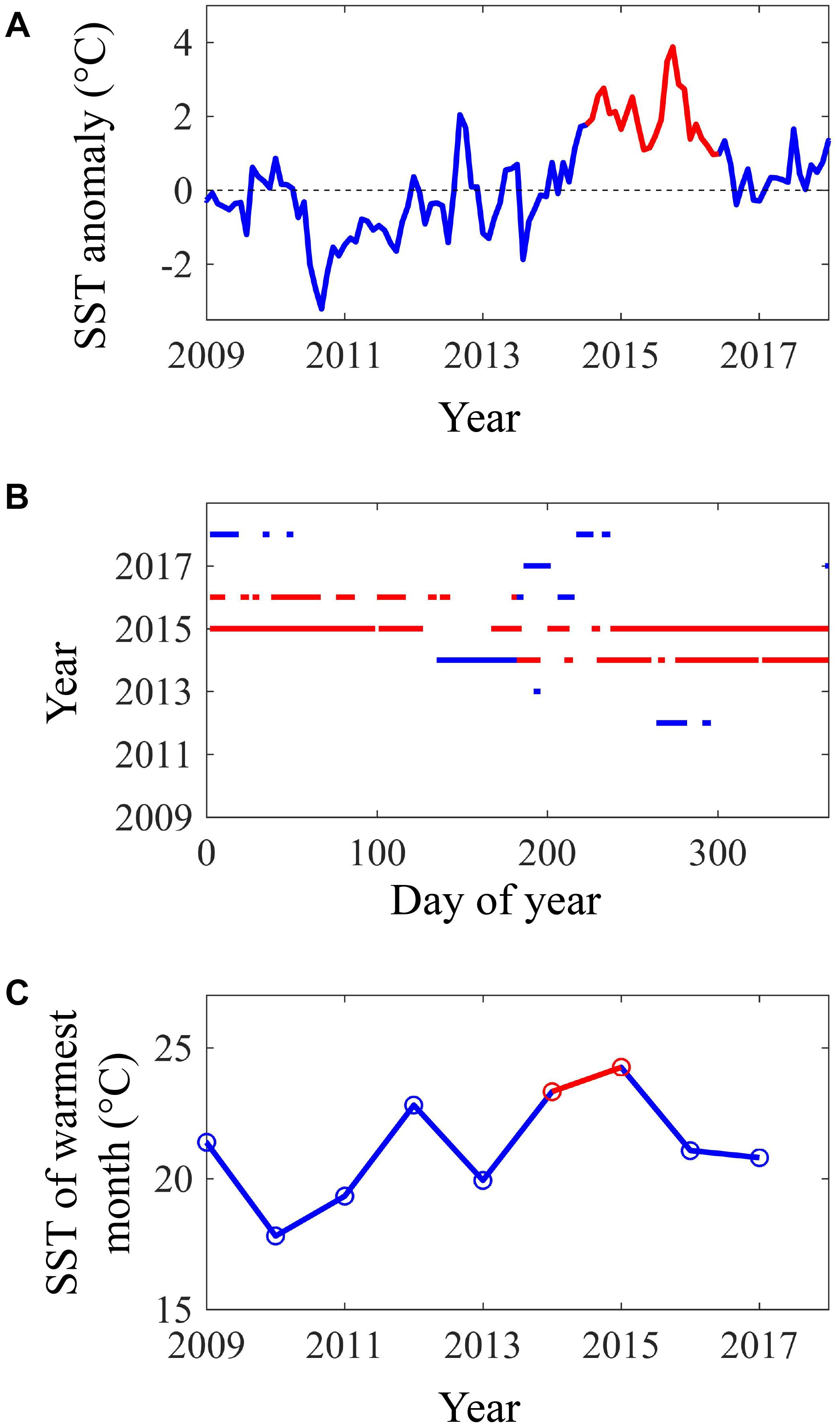
Figure 1. SST metrics from 2009 to 2018 averaged across the thirteen 100 km coastline segments that comprised the study area (27.1°N to 34.5°N): (A) monthly anomalies in SST, (B) occurrence and duration of heat waves, and (C) SST of the warmest month of each year. The 2014–2016 warm anomaly is shown in red.

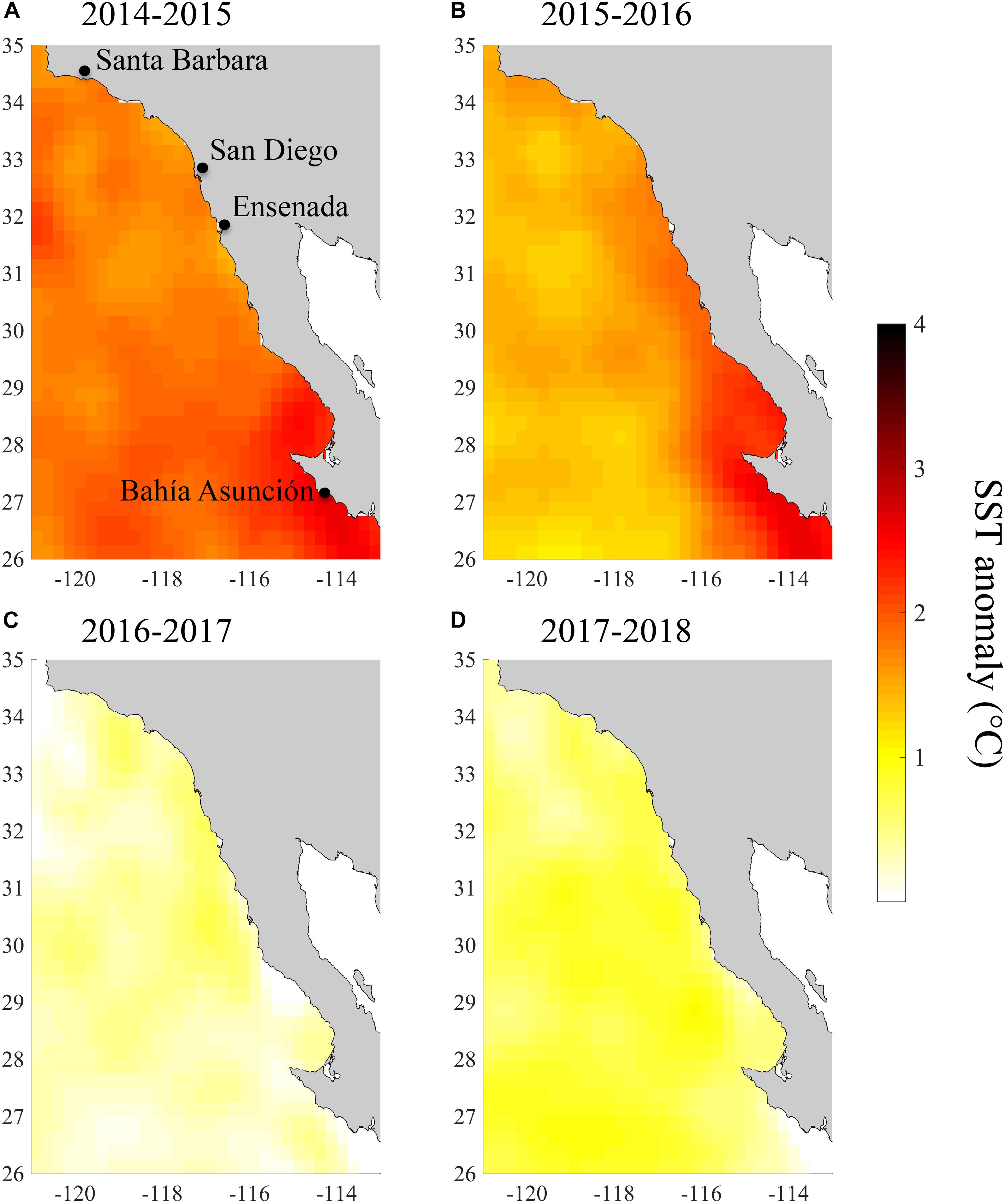
Figure 2. Mean SST anomalies across the study region for (A) July 2014–June 2015, (B) July 2015–June 2016, (C) July 2016–June 2017, and (D) July 2017–June 2018.

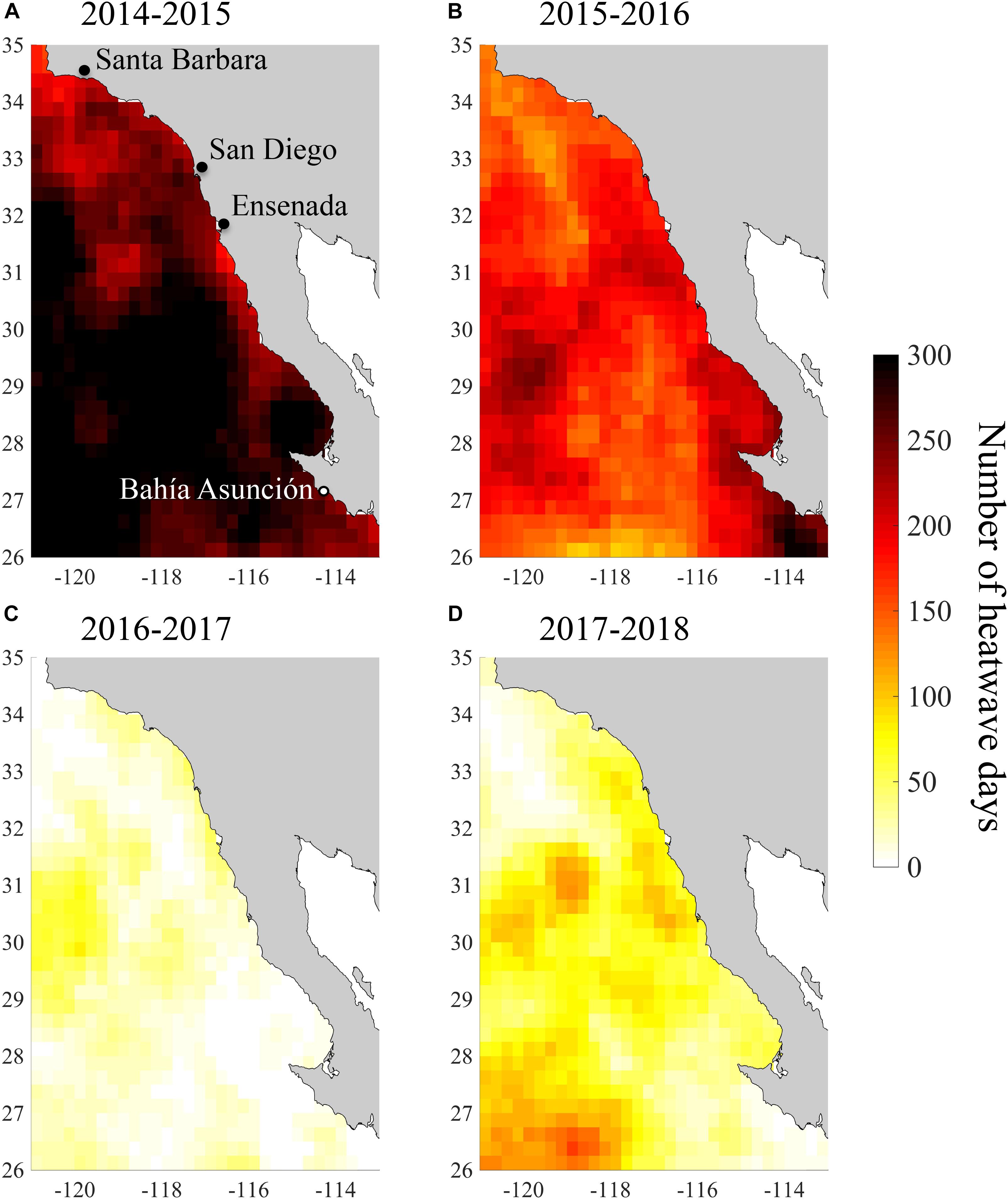
Figure 3. Total number of heatwave days across the study region for (A) July 2014–June 2015, (B) July 2015–June 2016, (C) July 2016–June 2017, and (D) July 2017–June 2018.

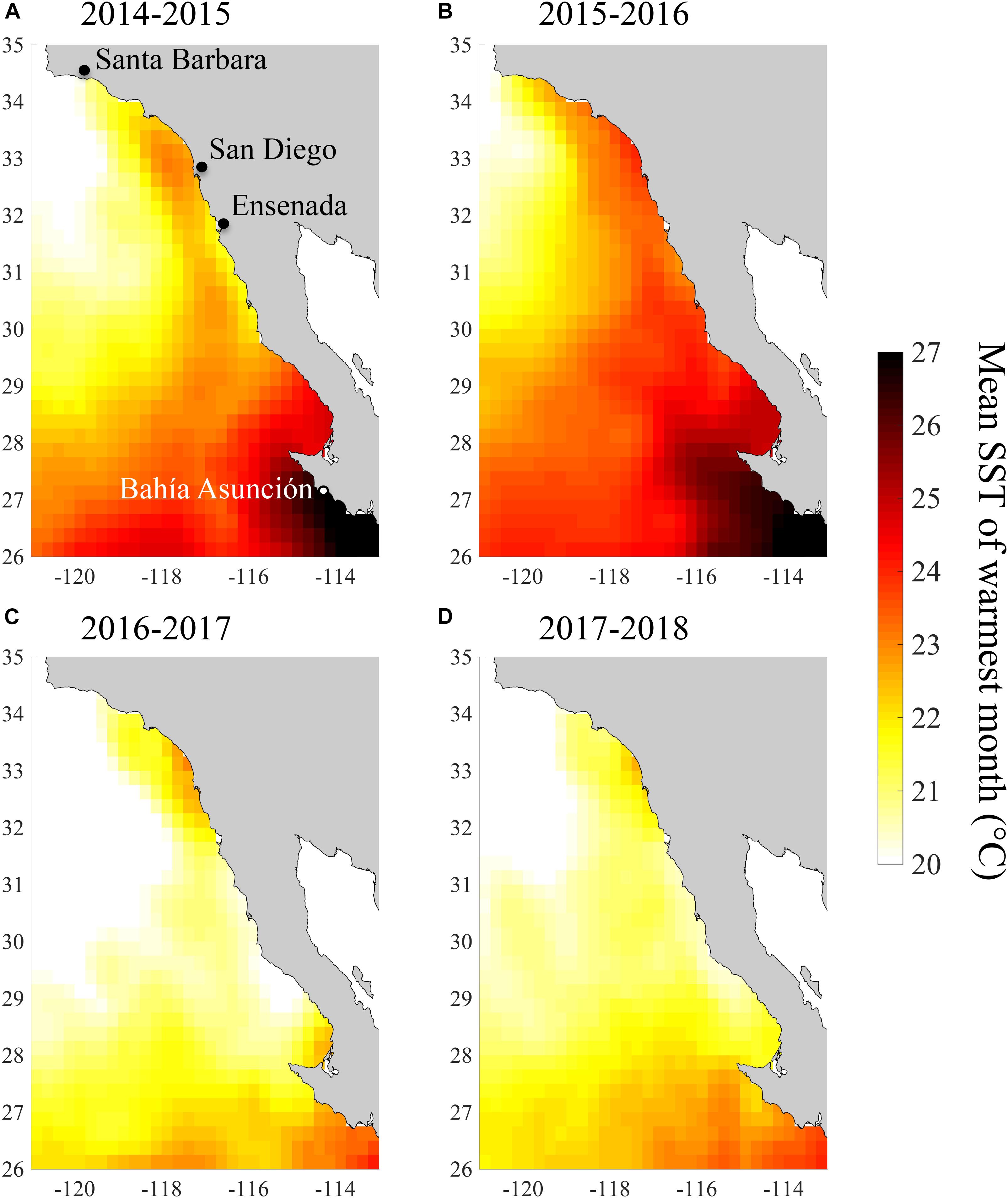
Figure 4. Mean SST of the warmest month across the study region for (A) July 2014–June 2015, (B) July 2015–June 2016, (C) July 2016–June 2017, and (D) July 2017–June 2018.

By the summer of 2016, SST returned to more normal conditions across our study area (Figures 2C, 4C). In 2016/2017 SST anomalies and heatwave days averaged 0.3°C and 21 days, respectively. The temperature of the warmest month similarly, declined across the study region from 2015/2016 to 2016/2017 (Figure 4C). However, temperature in the San Diego region (33°N) remained high (warmest month = 22.5°C) in 2016/2017 relative to all of the other coastline segments except the southernmost segment at Bahía Asunción (22.6°C). By comparison the temperature of the warmest month in Northern Baja (30.5°N–32°N) was 20.6°C in 2016/2017 (Figure 4D).

Spatiotemporal Variability in Giant Kelp Canopy Biomass

Giant kelp canopy biomass exhibited high intra- and inter-annual variability throughout the study region during the 5-year period prior to the onset of the heatwave in 2014. Seasonal patterns varied from year to year, but in most of the coastline segments, canopy biomass was typically highest in the spring or summer and lowest in winter (blue lines in Figure 5). These seasonal patterns were likely due to wave disturbance, which is typically strongest during the winter across most of our study area (Reed et al., 2011; Bell et al., 2015). However, during the heatwave this seasonal pattern changed, as canopy biomass in all the coastline segments reached minimums in the summer and fall of 2014 (Figure 5). Interestingly, in most regions this decline in kelp was followed by rapid recovery during the winter and spring of 2015, even though SST anomalies remained high with persistent heatwaves during this period (Figures 2, 3). This winter/spring recovery did not occur in the southern portions of the range (south of 30°N; Figures 5K–M) or in the coastline segment centered at 33.5°N, just north of San Diego (Figure 5D).

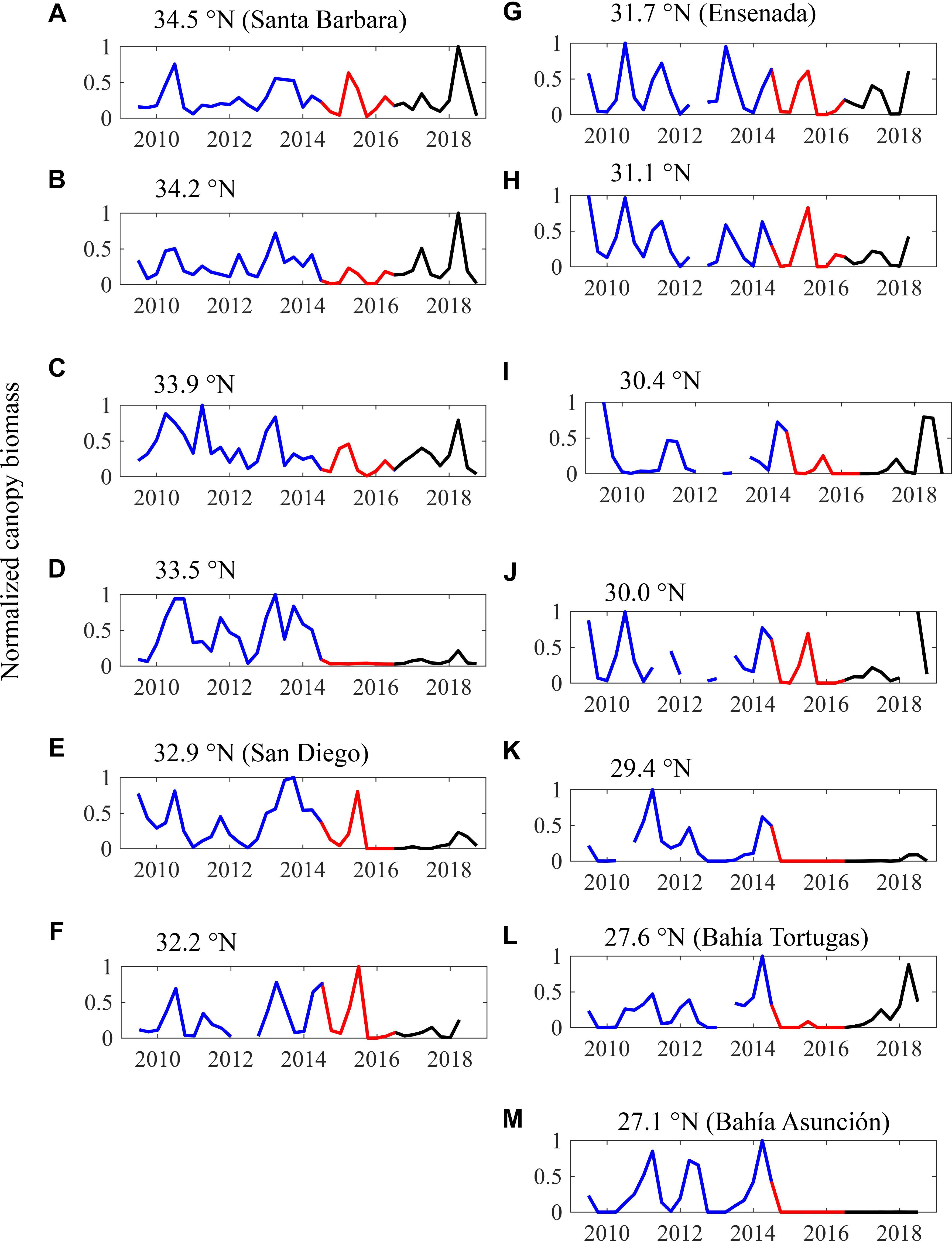
Figure 5. (A–M) Time series of seasonal giant kelp canopy biomass from 2009 to 2018 for the thirteen 100 km coastline segments. Biomass is normalized to the maximum biomass observed in a segment over the time series. The baseline period (July 2009–June 2014) is shown in blue, the heat wave period (July 2014–June 2016) is shown in red, and the recovery period (July 2016–December 2018) is shown in black.

Kelp canopy declined rapidly across all coastline segments during the summer and fall of 2015 (Figure 5). Recovery from this decline during the following winter and spring was less prevalent, and mean canopy biomass in 2015/2016 was lower than it had been in 2014/2015 for all but one coastline segment (Figure 6). During this period, the coastline segment near San Diego and Baja segments south of 29.5°N experienced a near complete loss of kelp canopy. The only two segments where kelp canopy biomass remained near the 2009–2013 average were Santa Barbara (34.5°N) and Ensenada (31.5°N).

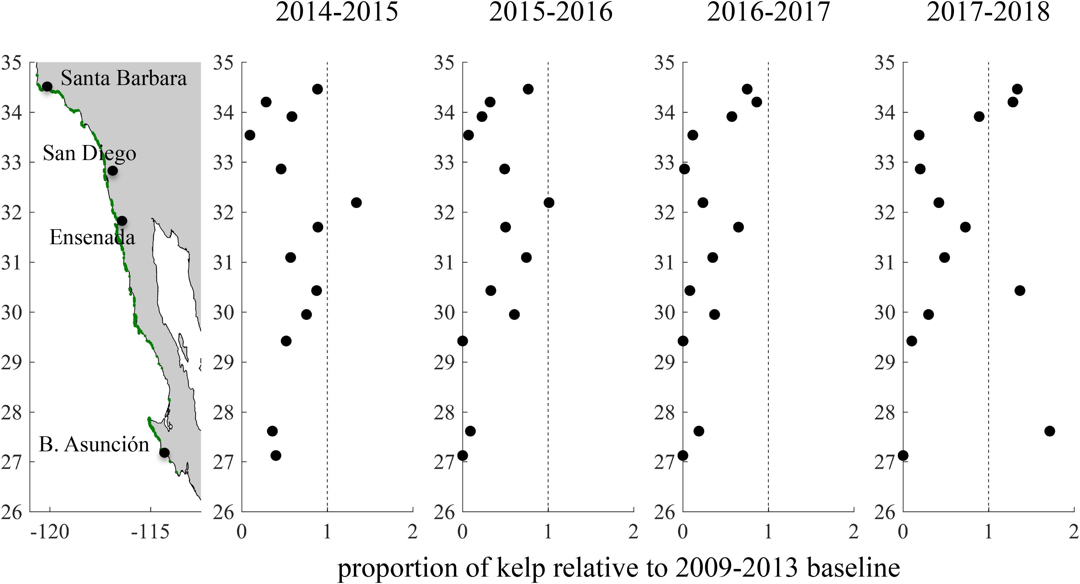
Figure 6. Change in kelp canopy biomass in southern and Baja California during and after the 2014–2016 warm period. For each year, mean giant kelp canopy biomass from July to June was divided by the mean canopy biomass between 2009 and 2013.

In the summer of 2016 the positive SST anomalies abated (Figure 2C), and kelp canopy biomass started to recover in the northern coastline segments (>33.5°N). However, kelp canopy biomass continued to decline in 2016/2017 across much of the rest of study area, particularly in northern Baja between 33° and 29°N (Figures 5, 6). Canopy biomass remained close to 0 near San Diego and in the southernmost portion of the range (<29.5°N).

Recovery of giant kelp canopy biomass in 2017/2018 showed a high degree of spatial variability. In the northernmost portions of our study area (>34.0°N), kelp canopy biomass continued its recovery from the previous year, and reached levels even higher than the 2009–2013 average (Figure 6). Canopy biomass near San Diego increased slightly from 2016/2017, but remained at historically low levels. In northern Baja, canopy biomass increased, but was still below baseline levels in all but one segment. Surprisingly, we documented a dramatic increase in kelp canopy in the southern portion of our study area near Bahía Tortugas (27.5°N). Canopy biomass in this coastline segment increased nearly 10-fold between 2016/2017 and 2017/2018, and by 2017/2018 canopy biomass was 1.7 × greater than the 2009–2013 baseline. By contrast, canopy biomass in the adjacent southernmost coastline segment near Bahía Asunción remained close to 0.

Giant Kelp Resistance and Resilience

The timing of canopy loss varied across our study area, and in most segments there appeared to be a delayed response to the onset of the heatwave in summer 2014. Only one of the 13 coastline segments experienced its lowest kelp canopy biomass during the first year of the heatwave (2014/2015). Six segments reached their minimums in 2015/2016, five in 2016/2017, and one in 2017/2018 (Supplementary Table S1). On average, annual canopy biomass was 40% of the baseline in 2015/2016 and 32% of baseline in 2016/2017. Resistance to the heatwave (i.e., the lowest annual canopy biomass relative to the average of the 5-years prior to the heatwave) ranged from 0 to 0.75 (mean = 0.23). There was a significant negative relationship (p < 0.05) between giant kelp resistance and both the number of heatwave days and the mean SST of the warmest month between July 2014 and June 2016 (Figure 7). The absolute metric, mean SST of the warmest month, was the best predictor of resistance based on model AIC, explaining approximately 41.3% of the variability in spatial patterns of kelp resistance (Table 1).

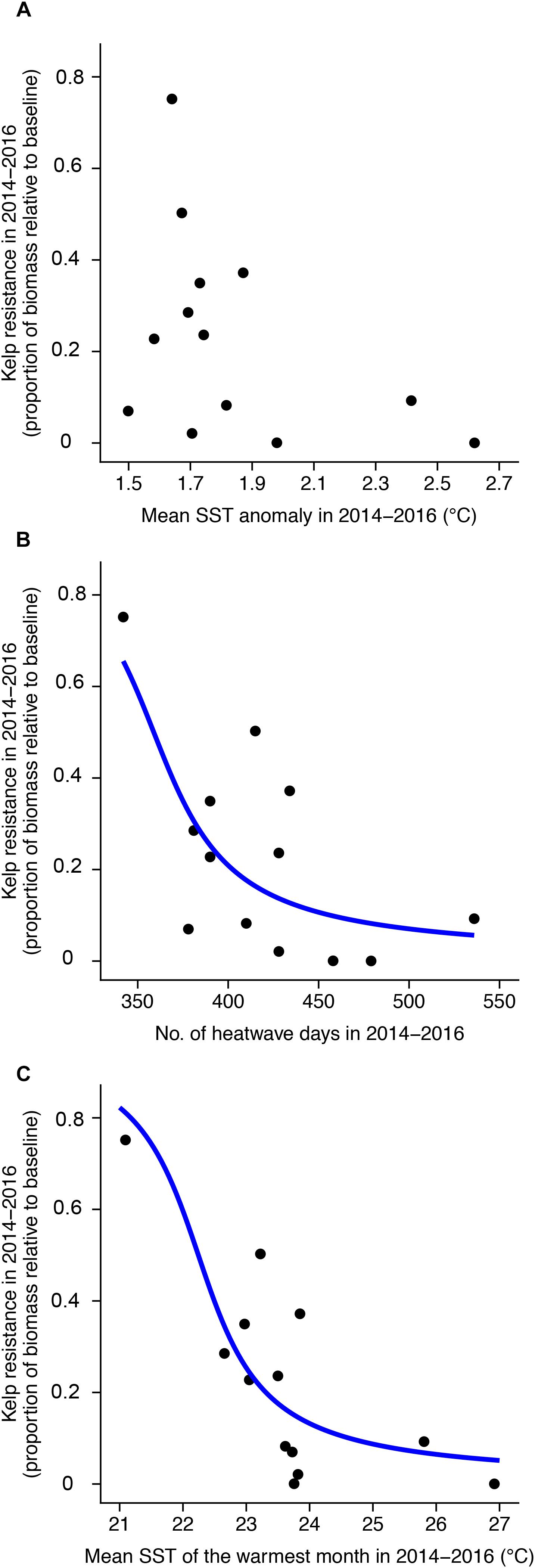
Figure 7. Relationship between kelp resistance and 2014–2016 sea surface temperature metrics: (A) SST anomaly, (B) number of heatwave days, and (C) mean SST of the warmest month. Blue lines show beta regression model fits for significant relationships (p < 0.05).

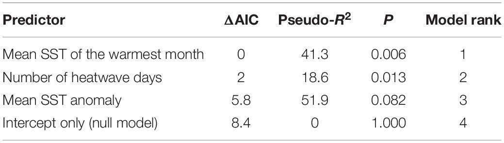
Table 1. Summary of model comparisons examining the relationship between giant kelp resistance and the three SST metrics from July 2014 to June 2016.

Kelp resilience (i.e., the proportion of canopy biomass in 2017/2018 relative to the 2009–2013 baseline) ranged from 0 to 1.7 (mean = 0.69) across all coastline segments. Resilience was not significantly correlated with any of the SST metrics calculated during (2014/2015–2015/2016) or after (2016/2017–2017/2018) the heatwaves (p > 0.35), suggesting that the severity of warming did not affect recovery (Figure 8 and Supplementary Figure S2, and Table 2). The resilience of the two southernmost coastline segments at Bahía Tortugas and Bahía Asunción are notable in that their resilience differed dramatically despite being adjacent to each other. Both of these segments experienced high SST during the 2014–2016 heatwave, but Bahía Asunción exhibited the lowest resilience of any coastline segment while Bahía Tortugas showed the highest.

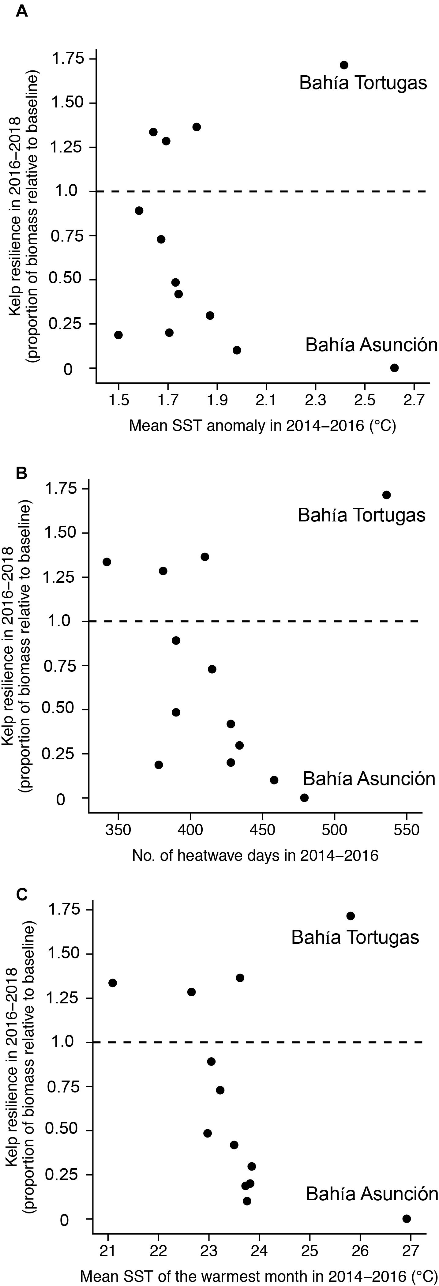
Figure 8. Relationship between giant kelp resilience and 2014–2016 sea surface temperature metrics: (A) SST anomaly, (B) number of heatwave days, and (C) mean SST of the warmest month.

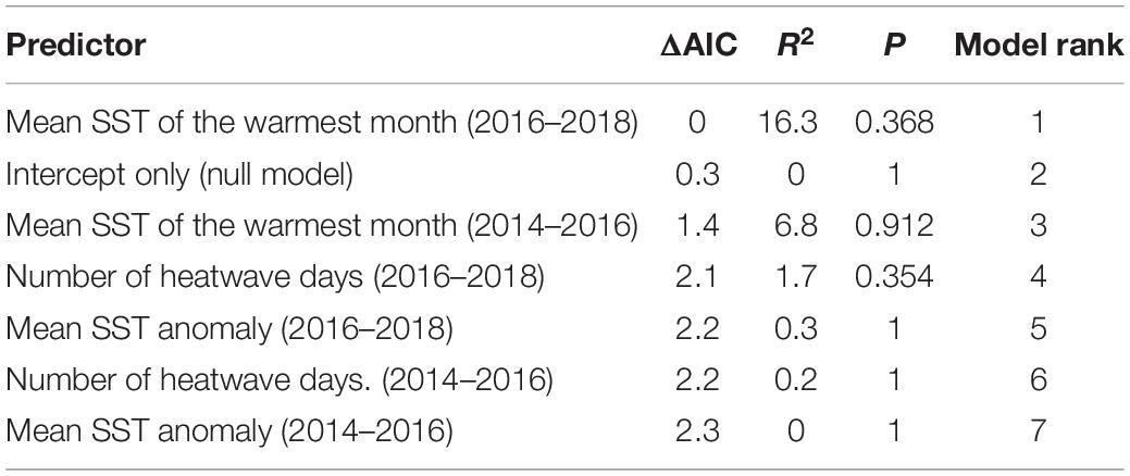
Table 2. Summary of model comparisons evaluating the relationship between giant kelp resilience and the three SST metrics during (July 2014 to June 2016) and after (July 2016 to June 2018) the heatwave.

Discussion

The exceptional warming of 2014–2016 had unexpected impacts on giant kelp abundance in southern and Baja California. Kelp canopy biomass declined at the onset of the heatwave in 2014 throughout the entire study region, however, the magnitude of this decline and the subsequent recovery varied dramatically and inconsistently with latitude. Several coastline segments showed an immediate decline in kelp abundance with little signs of recovery 2 years after the heatwave ended, including the segment at the southern range limit. In contrast, many of the coastline segments experienced a relatively strong recovery in spring 2015. This recovery was short-lived, however, and was followed by a sharp decline in the summer and fall of 2015. The specific reasons for the recovery of the canopy at these locations during the middle of the heatwave and its subsequent decline following the cessation of the heatwave remain unknown.

The variability in patterns of kelp resistance that we documented for the 2014–2016 heatwave differs substantially from the immediate and near complete loss of giant kelp observed throughout southern and Baja California during the heatwaves associated with the 1982/1983 and 1997/1998 El Niño events (Dayton and Tegner, 1989; Edwards and Estes, 2006). Both of these previous heatwaves were associated with catastrophic wave disturbance (Griggs and Brown, 1998), which caused the initial large-scale mortality in giant kelp populations throughout southern and Baja California, with warm, nutrient limited conditions negatively impacting subsequent recovery in some locations (Dayton and Tegner, 1984; Edwards, 2004; Edwards and Estes, 2006). The 2014–2016 heatwave was not associated with major wave disturbance (Reed et al., 2016), which likely explains the greater variability in the initial response and recovery of giant kelp that we observed. Near the southern range limit of giant kelp, high temperatures and/or low nutrients may have been severe enough in 2014/2015 to cause rapid mortality of adult giant kelp and suppress Subsequent recruitment. However, in northern Baja and most of southern California, some kelp survived the first year of the heatwave, and conditions were suitable for recruitment and/or regrowth of the canopy by the summer of 2015.

The delayed reaction of giant kelp to the warm anomaly across much of our study area may indicate that a major part of the heatwave’s impact was on giant kelp recruitment. Previous studies have identified “recruitment windows,” where spore release coincides with suitable temperature, nitrate, and irradiance conditions (Deysher and Dean, 1986). Environmental conditions may have been suitable for recruitment across parts of our study area in the winter and spring of 2015, which would explain the recovery observed during this period in many segments (Figure 5). Alternatively, it is possible that observed declines in canopy biomass during the summer and fall of 2014 resulted from a prolonged dieback of the canopy without mortality of plants below the surface. This canopy dieback was then followed by canopy recovery from surviving plants when conditions briefly improved in early 2015. The low rates of canopy recovery observed during the spring of 2016 when cooler temperatures prevailed suggests low adult densities and widespread recruitment failure during this time. That lack of recruitment in spring 2016 would have led to low adult abundance and sparse kelp canopies during the following year (2016/2017). While we cannot directly observe subsurface dynamics with our satellite data, the prolonged (>12 months in some segments) and widespread lack of canopy recovery after the heatwave ended in early 2016 is consistent with the hypothesis that canopy loss was the result of kelp mortality and not simply canopy dieback because giant kelp typically regrows its surface canopy within 6 months (Schiel and Foster, 2015).

The spatial patterns of resistance in giant kelp were better explained by an absolute thermal threshold (i.e., mean SST of the warmest month) than by relative increases in temperature as measured by SST anomalies and heatwave days. This finding contradicts that of Smale et al. (2019), who found that variation in the canopy biomass of giant kelp in our study region was best explained by the number of heatwave days. This contradiction in findings is likely related to confounding effects of wave disturbance. The negative relationship between canopy biomass and heatwave days observed by Smale et al. (2019) resulted primarily from low biomass during the exceedingly warm 1982–83 and 1997–98 El Niño events, which as noted above resulted from extremely large waves rather than warm water. Our finding that kelp was more responsive to an absolute temperature maximum than to the magnitude of relative temperature change suggests that local adaptation to heat stress did not have a major impact on the response of kelp to this warming event throughout much of its range.

Relative temperature metrics have been shown to explain variability in resistance to heat stress in other marine systems. For example, coral reef bleaching has been correlated with degree heating weeks, a relative metric calculated using the baseline climatology of a given location (Hughes et al., 2017). Coral reefs consist of an assemblage of different coral species, which may give them a higher capacity for local adaptation than ecosystems where the foundation species is a single species. However, relative temperature anomalies also explained variability in growth, survivorship, and reproduction across the distribution of Scytothalia dorycarpa, a temperate fucoid alga common to western Australia (Bennett et al., 2015). It is important to note that our results do not rule out the possibility that local adaptation may play an important role in controlling giant kelp dynamics. Instead, we suggest that there may be some absolute threshold beyond which local adaptation to temperature stress or nutrient limitation is no longer effective, and the 2014–2016 warming event exceeded that threshold throughout much of southern and Baja California.

Disentangling the effects of heat stress and nutrient limitation on giant kelp during heatwaves is challenging because temperature and nitrate concentration are strongly negatively correlated in the California Current system (Zimmerman and Kremer, 1984). Other sources of nitrogen are unrelated to temperature (e.g., ammonium and urea) and help to sustain kelp during warm periods when nitrate concentrations are low (Brzezinski et al., 2013; Smith et al., 2018). These other forms of nitrogen help account for the relatively high growth rates maintained by giant kelp (>2% dry mass per day) that we observed at our long-term study sites near Santa Barbara during the 2014–2016 heatwave (Rassweiler et al., 2018) despite positive temperature anomalies >4°C. Thus, it seems reasonable that heat stress rather than nutrient stress caused giant kelp to display its lowest resistance at locations with the highest temperatures. This contention is supported by our finding that most coastline segments where the mean SST of the warmest month during the 2014–2016 heatwave approached or exceeded 24°C suffered near-complete loss of giant kelp canopy, whereas those that did not exceed this threshold exhibited less kelp loss. Experimental studies have found that water temperatures >24°C exceed giant kelp’s physiological tolerance, leading to rapid mortality (Clendenning, 1971; Rothäusler et al., 2011). Similar patterns of kelp loss were observed near the southern range limit of giant kelp during the summer of 1997 when SST reached 25°C for 2 months, leading to a complete loss of both canopy and subsurface kelp at Bahía Tortugas (Ladah et al., 1999).

Recovery of kelp after the heatwaves was spatially variable and not related to any of the SST metrics that we analyzed. We observed high levels of resilience in the coastline segments in the north of our study area (>34°N) and in certain parts of Baja. Surprisingly, the most resilient coastline segment was in Bahía Tortugas (27.5°N), which is close to the southern range limit of giant kelp. This is in sharp contrast to the adjacent coastline segment at the southern range edge, which did not have any detectable kelp canopy by mid-2018, 2 years after the heatwave subsided. Kelp canopy biomass also remained well below baseline levels near San Diego (32.9°N). The Bahía Tortugas segment showed high levels of resilience, even though absolute and relative SST were high during the heatwave period. The area near Bahía Tortugas is characterized by strong localized coastal upwelling (Dawson, 1951; Woodson et al., 2018), which may have reduced heat and nutrient stress and promoted canopy regrowth and recruitment during and after the heatwave. Some of this small-scale temperature variability may not have been captured by our relatively coarse SST data. Other studies have reported rapid recovery of kelp in Bahía Tortugas following previous heatwaves (Ladah et al., 1999; Edwards and Estes, 2006), and this area could serve as an important refuge for giant kelp near its southern range edge following extreme warming events.

Biological processes such as dispersal, recruitment, competition, and grazing influence giant kelp population dynamics, and likely interact with environmental controls to explain local variability in resilience. For example, highly isolated giant kelp populations have lower persistence and resilience due to diminished demographic connectivity (Reed et al., 2006; Castorani et al., 2015, 2017) and, in some locations, inbreeding depression (Raimondi et al., 2004). Likewise, competition with understory algae can inhibit giant kelp recruitment (Reed and Foster, 1984; Reed, 1990), thereby negatively impacting population recovery following disturbance from warm temperatures or large waves (Edwards and Hernández-Carmona, 2005). Grazing by herbivores can have a strong impact on giant kelp abundance, and so spatial variability in grazing pressure due to processes such as top-down trophic controls may also influence resilience (Shears and Babcock, 2002; Lafferty, 2004; Ling et al., 2009). Interactions among environmental and biological processes may also be important, as increased temperatures can make kelp forests more vulnerable to other physical or biotic disturbance (Wernberg et al., 2010).

Our results highlight both the resilient nature of giant kelp in southern and Baja California, as well as the limits of that resilience. Populations near the equatorial range limit of giant kelp, which exist near temperature tolerance thresholds, are likely the most vulnerable to future increases in the frequency of marine heatwaves. However, marine microclimates, such as regions of localized upwelling, may provide spatial refuges from heatwaves that help repopulate neighboring areas following these disturbances. Other stressors, such as wave disturbance and grazing, may interact with positive temperature anomalies, and push giant kelp systems beyond their capacity for recovery. Interacting stressors may be especially important in the center of species distributions, where the system would otherwise be resilient to warming on its own.

Data Availability

The datasets generated for this study are available on request to the corresponding author.

Author Contributions

DR, KC, and TB conceived the study. KC and TB processed the satellite-based datasets. KC, DR, TB, and MC performed data analysis. KC wrote the first draft of the manuscript. All authors contributed substantially to revisions of the manuscript.

Funding

This research was supported by the U.S. National Science Foundation’s Long Term Ecological Research program (OCE 9982105, 0620276, 1232779 and 1831937) and the University of California Institute for Mexico and the United States (CN-17-177).

Conflict of Interest Statement

The authors declare that the research was conducted in the absence of any commercial or financial relationships that could be construed as a potential conflict of interest.

Supplementary Material

The Supplementary Material for this article can be found online at: https://www.frontiersin.org/articles/10.3389/fmars.2019.00413/full#supplementary-material

References

Alberto, F., Raimondi, P. T., Reed, D. C., Coelho, N. C., Leblois, R., Whitmer, A., et al. (2010). Habitat continuity and geographic distance predict population genetic differentiation in giant kelp. Ecology 91, 49–56. doi: 10.1890/09-0050.1
Alberto, F., Raimondi, P. T., Reed, D. C., Watson, J. R., Siegel, D. A., Mirari, S., et al. (2011). Isolation by oceanographic distance explains genetic structure for Macrocystis pyrifera in the Santa Barbara Channel. Mol. Ecol. 20, 2543–2554. doi: 10.1111/j.1365-294X.2011.05117.x
Banzon, V., Smith, T. M., Chin, T. M., Liu, C., and Hankins, W. (2016). A long-term record of blended satellite and in situ sea-surface temperature for climate monitoring, modeling and environmental studies. Earth Syst. Sci. Data 8, 165–176. doi: 10.5194/essd-8-165-2016
Bell, T. W., Allen, J. G., Cavanaugh, K. C., and Siegel, D. A. (2018). Three decades of variability in California ’ s giant kelp forests from the Landsat satellites. Remote Sens. Environ. (in press). doi: 10.1016/j.rse.2018.06.039
Bell, T. W., Cavanaugh, K. C., Reed, D. C., and Siegel, D. A. (2015). Geographical variability in the controls of giant kelp biomass dynamics. J. Biogeogr. 42, 2010–2021. doi: 10.1111/jbi.12550
Benjamini, Y., and Hochberg, Y. (1995). Controlling the false discovery rate: a practical and powerful approach to multiple testing. J. R. Stat. Soc. Ser. B 57, 289–300. doi: 10.1111/j.2517-6161.1995.tb02031.x
Bennett, S., Wernberg, T., Joy, B. A., De Bettignies, T., and Campbell, A. H. (2015). Central and rear-edge populations can be equally vulnerable to warming. Nat. Commun. 6:10280. doi: 10.1038/ncomms10280
Berkelmans, R., De’ath, G., Kininmonth, S., and Skirving, W. J. (2004). A comparison of the 1998 and 2002 coral bleaching events on the Great Barrier Reef: spatial correlation, patterns, and predictions. Coral Reefs 23, 74–83. doi: 10.1007/s00338-003-0353-y
Bond, N. A., Cronin, M. F., Freeland, H., and Mantua, N. (2015). Causes and impacts of the 2014 warm anomaly in the NE Pacific Nicholas. Geophys. Res. Lett. 42, 3414–3420. doi: 10.1002/2015gl063306
Brzezinski, M. A., Reed, D. C., Harrer, S., Rassweiler, A., Melack, J. M., Goodridge, B. M., et al. (2013). Multiple sources and forms of nitrogen sustain year-round kelp growth on the inner continental shelf of the Santa Barbara Channel. Oceanography 26, 114–123. doi: 10.5670/oceanog.2013.53
Burnham, K., and Anderson, D. (2002). Model Selection and Multimodel Inference: a Practical Information-Theoretic Approach, 2nd Edn. New York, NY: Springer-Verlag.
Castorani, M. C. N., Reed, D. C., Alberto, F., Bell, T. W., Simons, R., Cavanaugh, K. C., et al. (2015). Connectivity structures local population dynamics: a long-term empirical test in a large metapopulation system. Ecology 96, 3141–3152. doi: 10.1890/15-0283.1
Castorani, M. C. N., Reed, D. C., and Miller, R. J. (2018). Loss of foundation species: disturbance frequency outweighs severity in structuring kelp forest communities. Ecology 99, 2442–2454. doi: 10.1002/ecy.2485
Castorani, M. C. N., Reed, D. C., Raimondi, P. T., Alberto, F., Bell, T. W., Cavanaugh, K. C., et al. (2017). Fluctuations in population fecundity drive variation in demographic connectivity and metapopulation dynamics. Proc. R. Soc. B Biol. Sci. 284:20162086. doi: 10.1098/rspb.2016.2086
Cavanaugh, K., Siegel, D., Reed, D., and Dennison, P. (2011). Environmental controls of giant kelp biomass in the Santa Barbara Channel, California. Mar. Ecol. Prog. Ser. 429, 1–17. doi: 10.3354/meps09141
Chavez, F. P., Pennington, J. T., Castro, C. G., Ryan, J. P., Michisaki, R. P., Schlining, B., et al. (2002). Biological and chemical consequences of the 1997-1 998 El Nifio in central California waters. Prog. Oceanogr. 54, 205–232. doi: 10.1016/s0079-6611(02)00050-2
Clendenning, K. A. (1971). “Photosynthesis and general development in Macrocystis,” in The Biology of Giant Kelp Beds (Macrocystis) in California, ed. W. J. North (Lehre: Nova Hedwigia), 169–190.
Dawson, E. Y. (1951). A further study of upwelling and associated vegetation along Pacific Baja California. Mexico. J. Mar. Res. 10, 39–58.
Dayton, P. K., and Tegner, M. J. (1984). Catastrophic storms, El Niño, and patch stability in a southern California kelp community. Science 224, 283–285. doi: 10.1126/science.224.4646.283
Dayton, P. K., and Tegner, M. J. (1989). “Bottoms beneath troubled waters: benthic impacts of the 1982-1984 El Niño in the temperature zone,” in Global Ecological Consequences of the 1982–83 El Niño–Southern Oscillation, ed. P. W. Glynn (Amsterdam: Elsevier), 433–472. doi: 10.1016/s0422-9894(08)70045-x
Dayton, P. K., Tegner, M. J., Parnell, P. E., and Edwards, P. B. (1992). Temporal and spatial patterns of disturbance and recovery in a kelp forest community. Ecol. Monogr. 62, 421–445. doi: 10.2307/2937118
Deysher, L. E., and Dean, T. A. (1986). In situ recruitment of sporophytes of the giant kelp, Macrocystis pyrifera (L) C.A. Agardh: effects of physical factors. J. Exp. Mar. Biol. Ecol. 103, 41–63. doi: 10.1016/0022-0981(86)90131-0
Di Lorenzo, E., and Mantua, N. (2016). Multi-year persistence of the 2014/15 North Pacific marine heatwave. Nat. Clim. Change 6:1042. doi: 10.1038/nclimate3082
Edwards, M. S. (2004). Estimating scale-dependency in disturbance impacts: El Ninos and giant kelp forests in the northeast Pacific. Oecologia 138, 436–447. doi: 10.1007/s00442-003-1452-8
Edwards, M. S., and Estes, J. A. (2006). Catastrophe, recovery and range limitation in NE Pacific kelp forests: a large-scale perspective. Mar. Ecol. Prog. Ser. 320, 79–87. doi: 10.3354/meps320079
Edwards, M. S., and Hernández-Carmona, G. (2005). Delayed recovery of giant kelp near its southern range limit in the North Pacific following El Niño. Mar. Biol. 147, 273–279. doi: 10.1007/s00227-004-1548-7
Ferrari, S., and Cribari-Neto, F. (2004). Beta regression for modelling rates and proportions. J. Appl. Stat. 31, 799–815. doi: 10.1016/j.ijid.2019.06.017
García, L. V. (2004). Escaping the Bonferroni iron claw in ecological studies. Oikos 105, 657–663. doi: 10.1111/j.0030-1299.2004.13046.x
Graham, M. H., Vásquez, J. A., and Buschmann, A. H. (2007). Global ecology of the giant kelp Macrocystis: from ecotypes to ecosystems. Oceanogr. Mar. Biol. Annu. Rev. 45, 39–88.
Griggs, G. B., and Brown, K. M. (1998). Erosion and shoreline damage along the central California Coast: a comparison between the 1997-98 and 1982-83 ENSO winters. Shore Beach 66, 18–23.
Hijmans, R. J. (2016). Geosphere: Spherical Trigonometry. R package Version 1.5-5. Available at: https://cran.r-project.org/package=geosphere (accessed February 26, 2019).
Hobday, A. J., Alexander, L. V., Perkins, S. E., Smale, D. A., Straub, S. C., Oliver, E. C. J., et al. (2016). A hierarchical approach to defining marine heatwaves. Prog. Oceanogr. 141, 227–238. doi: 10.1016/j.pocean.2015.12.014
Hodgson, D., McDonald, J. L., and Hosken, D. J. (2015). What do you mean, ‘resilient’? Trends Ecol. Evol. 30, 503–506.
Howells, E. J., Beltran, V. H., Larsen, N. W., Bay, L. K., Willis, B. L., and Van Oppen, M. J. H. (2011). Coral thermal tolerance shaped by local adaptation of photosymbionts. Nat. Clim. Change 2, 1–5.
Hughes, T. P., Baird, A. H., Bellwood, D. R., Card, M., Connolly, S. R., Folke, C., et al. (2003). Climate change, human impacts, and the resilience of coral reefs. Science 301, 929–934.
Hughes, T. P., Kerry, J. T., Álvarez-Noriega, M., Álvarez-Romero, J. G., Anderson, K. D., Baird, A. H., et al. (2017). Global warming and recurrent mass bleaching of corals. Nature 543:373. doi: 10.1038/nature21707
Johansson, M., Alberto, F., Reed, D. C., Raimondi, P. T., Coelho, N. C., Young, M., et al. (2015). Seascape drivers of Macrocystis pyrifera population genetic structure in the northeast Pacific. Molecular 24, 4866–4885. doi: 10.1111/mec.13371
Johnson, C. R., Banks, S. C., Barrett, N. S., Cazassus, F., Dunstan, P. K., Edgar, G. J., et al. (2011). Climate change cascades: shifts in oceanography, species’ ranges and subtidal marine community dynamics in eastern Tasmania. J. Exp. Mar. Biol. Ecol. 400, 17–32. doi: 10.1016/j.jembe.2011.02.032
Kopczak, C. D., Zimmerman, R. C., and Kremer, J. N. (1991). Variation in nitrogen physiology and growth among geographically isolated populations of the giant kelp Macrocystis pyrifera (Phaeophyta). J. Phycol. 27, 149–158. doi: 10.1111/j.0022-3646.1991.00149.x
Ladah, L. B., and Zertuche-González, J. A. (2007). Survival of microscopic stages of a perennial kelp (Macrocystis pyrifera) from the center and the southern extreme of its range in the Northern Hemisphere after exposure to simulated El Niño stress. Mar. Biol. 152, 677–686. doi: 10.1007/s00227-007-0723-z
Ladah, L. B., Zertuche-González, J. A., and Hernández-Carmona, G. (1999). Giant kelp (Macrocystis pyrifera, Phaeophyceae) recruitment near its southern limit in Baja California after mass disappearance during ENSO 1997-1998. J. Phycol. 35, 1106–1112. doi: 10.1046/j.1529-8817.1999.3561106.x
Lafferty, K. D. (2004). Fishing for lobsters indirectly increases epidemics in sea urchins. Ecol. Appl. 14, 1566–1573. doi: 10.1890/03-5088
Ling, S. D., Johnson, C. R., Frusher, S. D., and Ridgway, K. R. (2009). Overfishing reduces resilience of kelp beds to climate-driven catastrophic phase shift. Proc. Natl. Acad. Sci. U.S.A. 106, 22341–22345. doi: 10.1073/pnas.0907529106
Miller, R. J., Lafferty, K. D., Lamy, T., Kui, L., Rassweiler, A., and Reed, D. C. (2018). Giant kelp, Macrocystis pyrifera, increases faunal diversity through physical engineering. Proc. R. Soc. B Biol. Sci. 285:20172571. doi: 10.1098/rspb.2017.2571
Moran, P. A. P. (1950). Notes on continuous stochastic phenomena. Biometrika 37, 17–23. doi: 10.1093/biomet/37.1-2.17
Oliver, E. C. J., Donat, M. G., Burrows, M. T., Moore, P. J., Smale, D. A., Alexander, L. V., et al. (2018). Longer and more frequent marine heatwaves over the past century. Nat. Commun. 9, 1–12. doi: 10.1038/s41467-018-03732-9
Paradis, E., Claude, J., and Strimmer, K. (2004). APE: analyses of phylogenetics and evolution in R language. Bioinformatics 20, 289–290. doi: 10.1093/bioinformatics/btg412
Pimm, S. L. (1984). The complexity and stability of ecosystems. Nature 307, 321–326. doi: 10.1038/307321a0
Raimondi, P. T., Reed, D. C., Gaylord, B., and Washburn, L. (2004). Effects of self-fertilization in the giant kelp, Macrocystis pyrifera. Ecology 85, 3267–3276. doi: 10.1890/03-0559
Rassweiler, A., Reed, D. C., Harrer, S. L., and Nelson, J. C. (2018). Improved estimates of net primary production, growth, and standing crop of Macrocystis pyrifera in Southern California. Ecology 99:2132. doi: 10.1002/ecy.2440
R Core Team (2019). R: A Language and Environment for Statistical Computing. Vienna: R Foundation for Statistical Computing. Available at: http://www.R-project.org/
Reed, D., Washburn, L., Rassweiler, A., Miller, R., Bell, T., and Harrer, S. (2016). Extreme warming challenges sentinel status of kelp forests as indicators of climate change. Nat. Commun. 7:13757. doi: 10.1038/ncomms13757
Reed, D. C. (1990). The effects of variable settlement and early competition on patterns of kelp recruitment. Ecology 71, 776–787. doi: 10.2307/1940329
Reed, D. C., and Foster, M. S. (1984). The effects of canopy shadings on algal recruitment and growth in a giant kelp forest. Ecology 65, 937–948. doi: 10.2307/1938066
Reed, D. C., Kinlan, B. P., Raimondi, P. T., Washburn, L., Gaylord, B., and Drake, P. T. (2006). A Metapopulation Perspective on Patch Dynamics and Connectivity of Giant Kelp. Marine Metapopulations. San Diego, CA: Academic Press.
Reed, D. C., Rassweiler, A., Carr, M. H., Cavanaugh, K. C., Malone, D. P., and Siegel, D. A. (2011). Wave disturbance overwhelms top-down and bottom-up control of primary production in California kelp forests. Ecology 92, 2108–2116. doi: 10.1890/11-0377.1
Rothäusler, E., Gomez, I., Hinojosa, I. A., Karsten, U., Tala, F., and Thiel, M. (2011). Physiological performance of gloating giant kelp Macrocystis pyrifera (Phaeophyceae): latitudinal variability in the effects of temperature and grazing. J. Phycol. 47, 269–281. doi: 10.1111/j.1529-8817.2011.00971.x
Sanford, E., and Kelly, M. W. (2011). Local adaptation in marine invertebrates. Annu. Rev. Mar. Sci. 3, 509–535. doi: 10.1146/annurev-marine-120709-142756
Schiel, D. R., and Foster, M. S. (2015). The Biology and Ecology of Giant Kelp Forests. Berkeley, CA: University of California Press.
Shears, N. T., and Babcock, R. C. (2002). Marine reserves demonstrate top-down control of community structure on temperate reefs. Oecologia 132, 131–142. doi: 10.1007/s00442-002-0920-x
Smale, D. A., Wernberg, T., Oliver, E. C. J., Thomsen, M., Harvey, B. P., Straub, S. C., et al. (2019). Marine heatwaves threaten global biodiversity and the provision of ecosystem services. Nat. Clim. Change 9, 306–312. doi: 10.1038/s41558-019-0412-1
Smith, J. M., Brzezinski, M. A., Melack, J. M., Miller, R. J., and Reed, D. C. (2018). Urea as a source of nitrogen to giant kelp (Macrocystis pyrifera). Limnol. Oceanogr. Lett. 3, 365–373. doi: 10.1002/lol2.10088
Storlazzi, C. D., and Griggs, G. B. (1996). Influence of El Niño-Southern oscillation (ENSO) events on the coastline of central California. J. Coast. Res. 26, 146–153.
Turner, M. G., Collins, S. L., Lugo, A. L., Magnuson, J. J., Rupp, T. S., and Swanson, F. J. (2003). Disturbance dynamics and ecological response: the contribution of long-term ecological research. BioScience 53, 46–56.
Wernberg, T., Smale, D. A., Tuya, F., Thomsen, M. S., Langlois, T. J., de Bettignies, T., et al. (2013). An extreme climatic event alters marine ecosystem structure in a global biodiversity hotspot. Nat. Clim. Change 3, 78–82. doi: 10.1038/nclimate1627
Wernberg, T., Thomsen, M. S., Tuya, F., Kendrick, G. A., Staehr, P. A., and Toohey, B. D. (2010). Decreasing resilience of kelp beds along a latitudinal temperature gradient: potential implications for a warmer future. Ecol. Lett. 13, 685–694. doi: 10.1111/j.1461-0248.2010.01466.x
Woodson, C. B., Espinoza, A., Monismith, S. G., Micheli, F., Hernandez, A., Torre, J., et al. (2018). Harnessing marine microclimates for climate change adaptation and marine conservation. Conserv. Lett. 12:e12609. doi: 10.1111/conl.12609
Zimmerman, R. C., and Kremer, J. N. (1984). Episodic nutrient supply to a kelp forest ecosystem in Southern California. J. Mar. Res. 42, 591–604. doi: 10.1357/002224084788506031
Zuur, A., Ieno, E., Walker, N., Saveliev, A., and Smith, G. (2009). Mixed Effects Models and Extensions in Ecology with R. New York, NY: Springer.
Zuur, A. F., and Ieno, E. N. (2016). A protocol for conducting and presenting results of regression-type analyses. Methods Ecol. Evol. 7, 636–645.
Keywords: giant kelp, resilience, Baja California (Mexico), heatwave, Southern California (United States)
Citation: Cavanaugh KC, Reed DC, Bell TW, Castorani MCN and Beas-Luna R (2019) Spatial Variability in the Resistance and Resilience of Giant Kelp in Southern and Baja California to a Multiyear Heatwave. Front. Mar. Sci. 6:413. doi: 10.3389/fmars.2019.00413
Received: 30 April 2019; Accepted: 04 July 2019;
Published: 23 July 2019.
Edited by:
Thomas Wernberg, The University of Western Australia, AustraliaReviewed by:
Ivan A. Hinojosa, Catholic University of the Most Holy Conception, ChileNeville Scott Barrett, University of Tasmania, Australia
Copyright © 2019 Cavanaugh, Reed, Bell, Castorani and Beas-Luna. This is an open-access article distributed under the terms of the Creative Commons Attribution License (CC BY). The use, distribution or reproduction in other forums is permitted, provided the original author(s) and the copyright owner(s) are credited and that the original publication in this journal is cited, in accordance with accepted academic practice. No use, distribution or reproduction is permitted which does not comply with these terms.
*Correspondence: Kyle C. Cavanaugh, kcavanaugh@geog.ucla.edu