Automated Detection Algorithm for SACZ, Oceanic SACZ, and Their Climatological Features
 Eliana Bertol Rosa
 Luciano Ponzi Pezzi
 Mario Francisco Leal de Quadro
 Nathaniel Brunsell
- 1Laboratory of Ocean Atmosphere Interaction, National Institute for Space Research, Earth Observation General Coordination, São José dos Campos, Brazil
- 2Department of Meteorology, Federal Institute of Santa Catarina, Florianópolis, Brazil
- 3Department of Geography and Atmospheric Science, University of Kansas, Lawrence, KS, United States
The South Atlantic Convergence Zone (SACZ) is responsible for a large amount of the total summer precipitation over Brazil and is related to severe droughts and extreme floods over the southeast of Brazil. This paper aims to demonstrate the feasibility of an objective, simplified and automated method based on satellite outgoing longwave radiation (OLR) for South Atlantic Convergence Zone (SACZ) and oceanic SACZ (SACZOCN) detection, and characterize their climatological features. Here we developed an automated algorithm and made available the SACZ and SACZOCN dates and characteristics (intensity and size) for the first time in the literature. The method agreed with 77% of SACZ occurrences compared with 21 years of SACZ observations. The temporal criterion of permanency of the SACZ convective activity for at least 4 days was essential to differentiate the SACZ from the transient frontal systems over the Brazilian Southeast. About 30% of the SACZ days occurred in November and March, therefore the December to February period is not sufficient to fully represent its activity. A barotropic trough near the Uruguay coast influences the intensity and position of the coastal and oceanic SACZ portions. When this trough closes into a cyclonic vortex Southwest of the SACZ (CVSS) cloud band it characterizes a SACZOCN episode. SACZOCN episodes were objectively identified, being characterized by a more intense convective activity and shifted to the north. We show that some oceanic SACZ episodes are associated with extreme floods and severe droughts over Brazil, therefore its identification is important to the Brazilian society. Besides, oceanic surface currents and temperature over the Southwestern Atlantic Ocean are modified during the SACZOCN active phase. The method presented here is a viable alternative to objectively classify SACZ and SACZOCN episodes, it can be implemented operationally and used to SACZ studies in the context of climate change.
1. Introduction
The tropical and subtropical regions of South America are characterized by a rainy season during the austral summer, with 50% of the total precipitation occurring between December and February (DJF) and 90% between November and March (Rao and Hada, 1990; Gan et al., 2004). The summer seasonal cycle starts with the development of the South America Monsoon System (SAMS) during spring (Zhou and Lau, 1998; Marengo et al., 2001), characterized by the development of a heat low over Gran Chaco at low levels, an upper tropospheric anticyclone (Bolivian High) and a trough east of it (Brazilian Northeastern trough; Kousky and Alonso Gan, 1981; Virji, 1981; Zhou and Lau, 1998). The South Atlantic Convergence Zone (SACZ) is part of the SAMS, being responsible for a great amount of the total precipitation over South America and associated with extreme rain events over Brazilian Southeast (Carvalho et al., 2002; Matos et al., 2014; Ambrizzi and Ferraz, 2015). In satellite cloud images it appears as a quasi-stationary cloud band, extending from the tropics toward the extra-tropics with a NW-SE orientation over South America and Southwestern Atlantic Ocean (Taljaard, 1972; Streten, 1973; Yassunary, 1977; Satyamurty and Rosa, 2019).
Kodama (1992, 1993) and Quadro (1994) diagnosed large-scale features of the SACZ. Among them are: (i) SACZ formation in the eastern side of a quasi-anchored trough of the subtropical jet, that penetrates into South America at ≈ 25°S and is localized near the Uruguay coast and (ii) low-level convergence and transport of moisture along the northeastern side of the trough, which increases low-level potential temperature and generates convective instability.
The symmetric source of latent heat, released in the Amazonian forest during the austral summer, was first pointed as the SACZ origin by Figueroa et al. (1995). Authors argued that the localized heat and Andes topography are responsible for the low-level trough near the Uruguay coast formation, in an orientation that resembles the SACZ. Gandu and Silva Dias (1998) investigated the role of the asymmetry in the source of heat during the SACZ active phase, caused by the substantial rain associated with southeastward displacement of the tropical convective activity. Gandu and Silva Dias (1998) results support the convective origin of the SACZ.
However, Kasahara and Silva Dias (1986) proposed that a tropical stationary source of heat can influence the intensity of the mid-to high latitudes planetary waves in the presence of a basic zonal flow with meridional and vertical shear. In the case described by Kasahara and Silva Dias (1986), the planetary wave response is barotropic in the mid-to high latitudes, including the region near the Uruguay coast. Grimm and Silva Dias (1995) showed via influence functions that anomalous upper-level divergence over the South Pacific Convergence Zone (SPCZ) region, related with a tropical stationary source of heat, is efficient in producing a cyclonic vorticity response in the Uruguay coast.
In summary, the intensity and position of the trough near the Uruguay coast are influenced by two main factors, the local latent heat released during the SACZ and remote sources of heat over the Pacific Ocean. The intensity and position of the trough near the Uruguay coast, in its turn, influences the intensity and position of convection associated with the coastal and oceanic SACZ regions, due to the compensatory ascending movement ahead of the trough.
In the last three decades, the SACZ has been detected by statistical and subjective (visual) methods, or a combination of them. Kodama (1992) used a visual-threshold criterion, where the SACZ must appear as a single cloud band in the high-cloudiness field and the cloud cover from 30 to 35°S must be > 4/10. Quadro (1994) on the other hand used a purely visual criterion that consists of selecting periods in which the satellite brightness temperature and observed precipitation data resembles the SACZ and remain persistent and intense for a minimum of 4 consecutive days.
A common statistical approach is to apply the empirical orthogonal function (EOF) or singular value decomposition (SVD) on the outgoing longwave radiation (OLR) field to find the mode associated with the SACZ, and select periods in the EOF or SVD time series that obey a threshold criterion (Nógues-Peagle and Mo, 1997; Barros et al., 2000; Jorgetti et al., 2014). Another common technique is to filter the OLR time series on a specific time scale and select periods with negative anomalies over South America and Southwestern Atlantic Ocean (SWAT) where the SACZ usually occurs (Liebmann et al., 1999; Cunningham and Cavalcanti, 2006).
Carvalho et al. (2002) selected days with the occurrence of OLR ⩽ 200 W m−2 adjacent pixels along the SACZ region (from the Amazonian forest to SWAT), necessarily crossing the Brazilian Southeast coastal region (their Figure 3). The authors did not consider a temporal criterion. Satyamurty and De Mattos (1989) suggested that the frontogenetic region over Brazilian Southeast is related with the SACZ origin via organization of the convective activity from the Amazon Basin to the SWAT during the frontogenesis. However, as pointed by Quadro (1994) and Siqueira and Toledo Machado (2004) only when the frontal system that passes over the Brazilian Southeast during summer organizes the tropical convection into a NW-SE oriented band for a period longer than 4 days it often characterizes the SACZ (i.e., not every frontal system is able to trigger a SACZ episode).
Recently, de Oliveira Vieira et al. (2013) and Ambrizzi and Ferraz (2015) proposed objective methodologies to detect SACZ-related extreme precipitating events considering temporal thresholds. Authors focused on specific regions of the SACZ, namely the southern Amazonia (de Oliveira Vieira et al., 2013) and the southeast of Brazil (Ambrizzi and Ferraz, 2015). The main idea of the precipitation based SACZ detection is to select consecutive days in which the precipitation stayed above a certain threshold, generally related to the climatological value of target areas (SACZ regions).
Precipitation along the SACZ can be of convective or stratiform nature. The precipitation over Amazonia is mostly from wide convective structures with a medium contribution of stratiform rain, the Brazilian Plateau presents a mix of deep and wide convective cores and the SWAT has mainly stratiform cloudiness with some wide convective cores (Romatschke and Houze, 2010, 2013). Wide convective cores (broad stratiform) are related with Mesoscale Convective Systems (MCSs) in the early (late) and strong (weak) convective stage of their life cycle, while deep convective cores represent isolated convection cells (Houze, 2004; Romatschke and Houze, 2010).
Lower values of OLR are commonly used as a proxy for strong convection and precipitation events (Kodama, 1992, 1999; Carvalho et al., 2002; Seo et al., 2008). In the SACZ region, negative OLR anomalies with respect to DJF long-term mean generally occur during periods of high level cloudiness (Liebmann et al., 1999) and large regions of OLR < 220 W m−2 are typically observed during enhanced cloud cover (Kiladis and Weickmann, 1992, 1997). Therefore, it is expected that by choosing an appropriate value and temporal criterion the OLR can satisfactorily represent the main types of precipitation throughout the SACZ cloud band and its stationarity.
The convection associated with the SACZ can be strong over its continental and/or oceanic portions. Intense convection over SACZ oceanic region is related to intensification and westward displacement of the subtropical barotropic jet trough. (Grimm and Silva Dias, 1995; Carvalho et al., 2002; Jorgetti et al., 2014). However, as far as our knowledge goes, there are no objective criteria to distinguish the continental and oceanic SACZ. This is a limitation of using precipitation based methods since rainfall observations are generally unavailable over oceanic regions. Satellite measurements of OLR, on the other hand, are available for both continental and oceanic regions.
This paper aims to demonstrate the feasibility of an objective, simplified and automatic method to detect SACZ episodes based on satellite measured OLR and, through it, determine quantitative characteristics and key synoptic features for both, SACZ and oceanic SACZ episodes. In addition, near surface variables related with ocean-atmosphere interaction in the SACZ region are analyzed. The paper is organized as follows, sections 2 and 3 present the data and methodology description, respectively, section 4 contains the results and discussion and the paper finishes with a summary and conclusions in section 5.
2. Data
The time period considered in the present work includes the austral summer months of November, December, January, February and March from 1996 to 2016, a total of 3,177 days.
The satellite product Daily Outgoing Longwave Radiation Climate Data Record (Daily OLR CDR) version v01r02 from NOAA was used for the algorithm development. The data are daily averages, updated daily, with 1 × 1° of spatial resolution and are available at https://www.ncdc.noaa.gov/cdr/atmospheric/outgoing-longwave-radiation-daily. This product was chosen because of the ability to combine the accuracy of a satellite polar sensor with the high temporal resolution of a geostationary one (Lee et al., 2004).
Precipitation from the Multi-Source Weighted-Ensemble Precipitation Version 2 (MSWEP V2) was used (Beck et al., 2019). Daily means were calculated from the 3-hourly available data at http://www.gloh2o.org/. The MSWEP V2 merges gauge, satellite, and reanalysis-based data to provide reliable precipitation estimates over the entire globe (Beck et al., 2019).
The other atmospheric and oceanic fields are from the Climate Forecast System re-analysis (CFSR) from 1996 until 2010 (Saha et al., 2010) and complemented by Climate Forecast System Version 2 (CFSv2) from 2011 until 2016 (Saha et al., 2011). Both are available at https://rda.ucar.edu/. The daily averages were obtained from the 6-hourly products with 0.5 × 0.5° of spatial resolution, except for the shortwave incident radiation where only the daily time scale was considered.
The SACZ analysis provided by the Brazilian Center for Weather and Climate Prediction (Centro de Previsão de Tempo e Clima, CPTEC-INPE) was used for statistical comparison with the SACZ dates found by the present objective method. Meteorologists from CPTEC-INPE visually identify the SACZ activity by checking if its spatial pattern remains for at least 4 days on orbital data of brightness temperature. SACZ visually detected dates are available on the monthly climate report (Climanálise Bulletin) at http://climanalise.cptec.inpe.br/~rclimanl/boletim/ and in Rosso et al. (2018) in table format.
It is worth mentioning that the visual methodology implemented by CPTEC-INPE has improved over time. Before 2005 many SACZ episodes were observed only on the satellite brightness temperature data. After 2005, in addition to the orbital image analysis, the following atmospheric fields also had to correspond to a SACZ spatial pattern: (i) 850 hPa divergence of water vapor flux and streamline; (ii) 500 hPa omega velocity and streamlines; (iii) 200 hPa mass divergence and streamlines and (iv) accumulated rain over the continent.
Synoptic analysis of a 21-days long SACZ episode as reported by Climanálise shows that at least 2 of these days were not SACZ days (Figure S1). Visual methods of classification are always subject to human interpretation. We conjecture that well-formulated objective classifications may be more reliable than the visual ones.
For the above mentioned reasons, the observed SACZ days are not considered in the present work as an absolute truth, which must be taken into account while evaluating the SACZ detection algorithm.
3. SACZ Detection Algorithm
The present section is organized as follows, first we present the algorithm parameters, followed by a description of the statistical methods used in the sensibility tests and it ends with the final form of the algorithm.
Figure 1 shows the OLR composite of a SACZ episode identified by Climanalise's meteorological group, where it is clear that the SACZ spatial pattern appears as a link of grid points with lower OLR values (shades of blue). The hypothesis that the OLR field mimics the SACZ signature in the satellite cloud images can be verified by comparing our Figure 1 with Figures 1 (lower panel) and 2 of Satyamurty and Rosa (2019). The algorithm was developed to identify SACZ episodes looking for convective contiguous regions in the daily OLR field over South America whose location, area, eccentricity, and temporal persistence correspond to the SACZ activity.
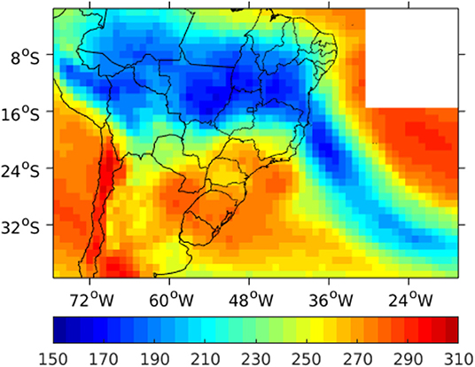
Figure 1. Spatial domain used in the classification algorithm. The upper right corner was removed to avoid the ITCZ convection influence. Mean OLR (W m−2) during the observed SACZ episode from 12 to 18 January, 2007.
The choice of these parameters was inspired in the work of Carvalho et al. (2002). The main differences are that we imposed a threshold for the area, eccentricity, location, and temporal permanence of the convective contiguous regions to classify a sequence of days as a SACZ episode (i.e., the shape and stationarity of the convective contiguous region must correspond to a SACZ pattern). Carvalho et al. (2002), on the other hand, considered every day with occurrence of OLR ⩽ 200 W m−2 adjacent pixels that cross the coastal SACZ region (their Figure 3 top panel), and then related the area, eccentricity and intensity of these convective contiguous regions with the atmospheric patterns over SA.
The spatial domain of the OLR daily field used by the algorithm is shown in Figure 1. The upper-right corner was removed to avoid confusion of the algorithm between the Intertropical Convergence Zone (ITCZ) convection and the SACZ convection. In the present algorithm there are two possible classes for each OLR image: (i) SACZ, that represents days of active SACZ and (ii) No-SACZ, that represents days of inactive SACZ.
The first step of the algorithm is to replace pixels with OLR values higher than a threshold with a Not a Number (NaN) flag, excluding non-convective pixels. Convective activity is generally represented by OLR ranging from 200 to 230 W m−2 (Kodama, 1992, 1999; Seo et al., 2008), with 200 W m−2 being associated with extreme precipitation events (Carvalho et al., 2002). Considering a 2D OLR field, this step can be expressed as:
In the second step a region growing image segmentation algorithm is applied. This algorithm is used to produce image segments that are formed by connecting adjacent pixels that obey a similarity measurement. A central pixel is connected with another eight pixels by its four sides and four corners. In our case, the adjacent pixels are joined in one segment of image if the OLR < threshold. After the application of the region growing algorithm the OLR image is divided into n segments and from now on we will refer to the n isolated image segments as convective segments (CSG(n)) on a given day.
The third step of the algorithm is to measure the size of each CSG(n), given by the number of pixels inside it. If the CSG(n) size is less than a threshold, then the CSG(n) is excluded (replaced with a NaN flag). The reason for this step is that smaller scale convective systems occur over South America during austral summer regardless of SACZ presence, like MCSs and isolated storms (Romatschke and Houze, 2010, 2013). To relate the CSG(n) size with the convective activity area, the number of pixels is multiplied by the pixel area (1 × 1° pixel corresponds to ≈ 12, 100 km2). This part of the code is written as follows:
The next steps of the algorithm were formulated using the general SACZ description, a continuous cloud band, organized and elongated in the NW-SE direction. We considered that this description is still true for the OLR field, as shown in Figure 1.
The fourth step of the algorithm is to verify if only one CSG(n) remains. If this condition is true the CSG(n) is considered as a SACZ candidate, otherwise the algorithm will consider it as a No-SACZ day. With this step, we guarantee that the convective activity is organized over South America during a SACZ candidate day. We can express this step as follows:
In case CSG(n) = SACZ, the fifth algorithm step is to verify if the CSG(n) crosses the Brazilian coastline at a given extent, given by the number of pixels occurring over it. Consider that CLi is the number of pixels of the CSG(n) occurring over the Brazilian coastline:
If this condition is true the CSG(n) remains as a SACZ candidate, otherwise, the algorithm will classify it as a No-SACZ day. With this step we guarantee that the cloud band is not confined in the Amazon region, or barely associated with the coastal and/or oceanic SACZ portions during a SACZ candidate day.
In case CSG(n) = SACZ, the sixth step is to use an eccentricity threshold to evaluate the elongation of the cloud band characteristic of SACZ. The eccentricity of the CSG(n) is the same as the ellipse in which the CSG(n) fits in. The ellipse eccentricity is defined as usual, , where a is the semi-major axis and b the semi-minor axis, with values varying from 0 (a perfect circle) to 1 (a linear segment). Considering that ECC is the eccentricity of the CSG(n), we can express this condition as follows:
The above mentioned steps are repeated for all time period (a total of 3177 OLR images). Finally, the temporal threshold is applied. If there are at least 4 consecutive days of CSG(n) = SACZ, these days are classified as a SACZ episode. If there are <4 consecutive days of CSG(n) = SACZ, these days are classified as No-SACZ days. The 4-days criterion is in accordance with Quadro (1994), Siqueira and Toledo Machado (2004), Ambrizzi and Ferraz (2015), and the observational data set used for comparison (from CPTEC-INPE).
In summary, we have four thresholds to define: (i) OLR, the OLR value in W m−2 that represents the convective activity; (ii) size of the CSG(n) given by its number of pixels that represents smaller scale convective systems (not related with the SACZ activity); (iii) CLi, the extent in which the CSG(n) must cross the Brazilian coastline given by the number of pixels of the CSG(n) that occur over it and (iv) ECC, the eccentricity (dimensionless) that the CSG(n) must have to remain as a SACZ candidate.
The algorithm was executed and evaluated against visual SACZ dates from CPTEC-INPE several times and sensitivity tests were done to improve the agreement between the algorithm and observational methodologies, as will be shown in the next subsection.
3.1. Statistical Evaluation of the SACZ Detection Algorithm
For the sake of simplicity, we will refer to the SACZ days detected by the automatic algorithm as automated SACZ, and the visual observations from Climanálise Bulletin as visual SACZ. We emphasize that the visual SACZ dates were not considered here as absolute truth, as explained in section 2. The automated SACZ dates in each algorithm run was evaluated against the visual ones with the help of a contingency table (Wilks, 1995).
In the present work, the contingency table of Wilks (1995) was used as follows, A is the hit of the automated SACZ in relation to the visual SACZ (i.e., when the SACZ day coincides in both methodologies), B is the false alarm (i.e., when an automated SACZ day do not coincides with a visual one), C represents the visual SACZ days that are not detected by the algorithm (i.e., when the algorithm considered a No-SACZ day but the visual method considered it as an active SACZ day) and D represents the correct rejections of the algorithm (when both methodologies agree with a No-SACZ day).
Following the methodology proposed by Fawcett (2005), true positives (TP) and false positives (FP) rates of automated SACZ days were calculated. They are defined as follows:
Finally, TP and FP were used to construct the receiver operating characteristics (ROC) graph, in which TP rate is plotted on the y-axis and FP on the x-axis [for further information about ROC analysis see Fawcett (2005)]. It is important to say that the sum of TP and FP is not equal to 100%, because they are calculated with respect to the marginal totals for visual SACZ (A + C and B + D), not the total number of days (N = A + B + C + D). In summary, TP = 1 means total agreement between the automated and visual SACZ for the active SACZ class, and FP = 0 means total agreement for the inactive SACZ class (No-SACZ).
The threshold values described in the above section were changed, one at a time, in several algorithm runs. For each run the contingency table was constructed and the TP and FP values were plotted in the ROC graph (Figure 2). Interpretation of Figure 2 is direct and simple, the “C” followed by a number represents the algorithm runs (SACZ classifications), the closest the algorithm run stays to the upper-left corner the bigger the agreement between automated and visual SACZ. This process was repeated until the change of the threshold values results in no decrease in the distance between the algorithm run and the upper-left corner of Figure 2. In total there were 25 runs (from C1 to C25 in Figure 2).
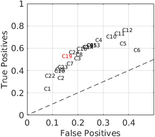
Figure 2. ROC graph of the 25 algorithm runs. Each run is represented by the letter C followed by the number of the run. The chosen run is highlighted in red (C19). The dotted line is the bisector, below which any classification is random. The more to the right (left) the greater (smaller) the disagreement between automated and visual SACZ days (i.e., false positives). The more to the top (bottom) the greater (smaller) the agreement between automated and visual SACZ days (i.e., true positives).
For the four thresholds described in the above section we tested the following values: (i) OLR ranging from 200 to 250 W m −2; (ii) size of the CSG(n) to be excluded ranging from 65 pixels (or 786.5 × 10³ km2) to 105 pixels (or 1270.5 × 103 km2); (iii) CLi ranging from 2 to 8 pixels (or ≈ 220 to 880 km of coastline) and (iv) ECC from 0.5 to 0.85. The detailed threshold values for each of the 25 algorithm runs are in the Table S1.
All algorithm runs stayed above the bisector line (Figure 2), meaning that none of them were random (the parameters of the algorithm are viable to detect the SACZ), as explained by Fawcett (2005). In the next two paragraphs we will show how the threshold values are related to the SACZ occurrence in nature, and what is the consequence of choosing different values during the classification process.
The C6 algorithm run position in Figure 2 shows that 45% of the automated SACZ were not visual SACZ days (FP = ≈ 0.41) and 60% of the automated SACZ were also visual SACZ (TP ≈ 0.6). In C6 the OLR threshold is 250 W m−2, which favors the formation of few and large convection segments (CSG(n)) by the region growing algorithm. The second condition is to exclude CSG(n) < 85 pixels (or 1.028 × 10⁶ km2), increasing the chance of the CSG(n) remaining as a SACZ candidate (if n = 1). In the next steps the CSG(n) have to cross the coastline in a narrow extensions (2 pixels, or 220 km), and it is allowed to have an almost circular shape (eccentricity threshold = 0.5). In summary, this algorithm configuration is very permissive, resulting in an accurate but not precise SACZ classification (i.e., high TP and FP rates).
The opposite situation occurs when the algorithm is very restrictive. In C1, for example, the OLR threshold is 200 W m−2 and the eccentricity equal to 0.5. In this case there were few automated SACZ days that did not match with the visual ones (FP ≈ 0.1), but the algorithm missed a lot of visual SACZ days (TP ≈ 0.2; i.e., the algorithm is precise but not accurate).
Besides the ROC analysis, three statistical metrics were calculated to chose the best algorithm run, bias (BI), hit rate (HR) and Euclidean distance (ED). As defined in Wilks (1995), BI and HR are respectively defined as:
Where A, B, C and D are the contingency table values and N is the total number of days. Here we considered BI = 1 − BI. The best BI value is 0, meaning no overestimation or underestimation in the number of automated SACZ days compared to the visual ones. BI greater (less) than 0 means underestimation (overestimation) of the automated SACZ days compared to the visual SACZ days. Note that BI says nothing about the correspondence between automated and visual SACZ, for this purpose we use HR. The best value for HR is 1, representing 100% of agreement between automated and visual SACZ days. The interpretation of the HR differs from FP and TP because HR is calculated in relation to the total of days (N), indicating the algorithm hit for both classes (SACZ and No-SACZ).
ED is the distance in the ROC graph between the position of the run and the upper-left corner (TP = 1 and FP = 0 in Figure 2), therefore the best value is zero. ED is defined as follows.
Table 1 shows that among the 25 algorithm runs C4 had the lowest ED, C19 agreed with observations the greater number of times (highest HR) and C24 had almost the same number of active SACZ days as the observation (lowest BI). The complete table with the parameter sets and statistical metrics for each algorithm run is in Table S1.
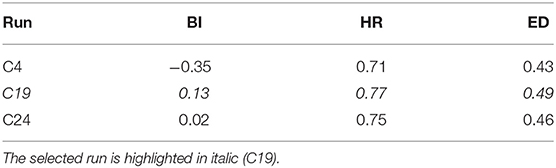
Table 1. Best algorithm runs according to bias (BI), hit rate (HR), and Euclidian Distance (ED) statistical metrics.
The C19 algorithm run was selected because it has the lowest FP rate (FP = 0.13) among the runs listed in Table 1 (i.e., only 13% of the automated SACZ did not agree with visual SACZ). Besides, C19 had about 77% of agreement with the observations for both classes, SACZ and No-SACZ (HR value in Table 1). In order to characterize dynamic and thermodynamic features of the SACZ occurrence it is important to have a small number of FP SACZ days.
A summary of how the algorithm works considering the selected run thresholds (C19) is shown in the flow chart of Figure 3. In Figure 3 the oval shapes represents starting and ending points of the algorithm. Boxes are individual steps and diamonds show the decision points (yes/no conditions).
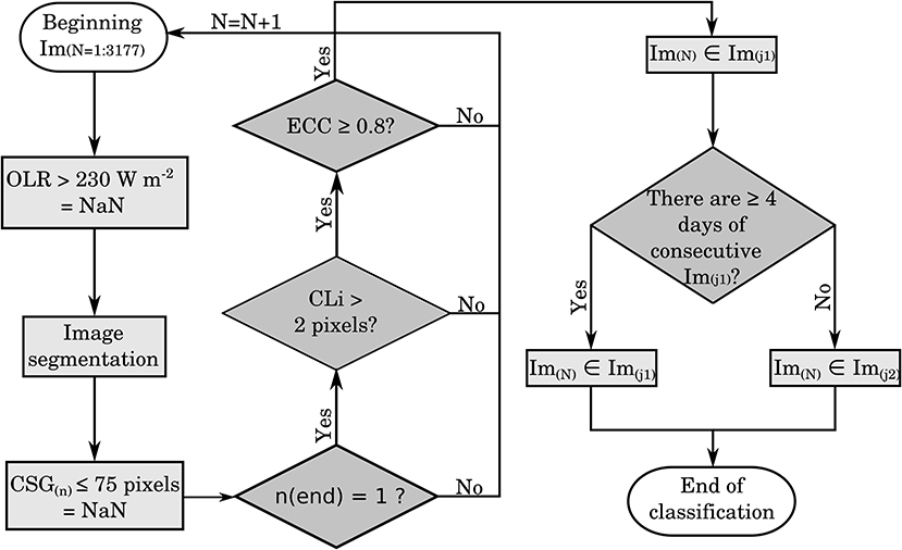
Figure 3. Flow chart of the algorithm steps. Oval shapes represents starting and ending points of the algorithm. Boxes are individual steps and diamonds show the decision points (yes/no conditions). N is the time index (a total of 3,177 daily OLR images processed), CSG(n) is the convective segment candidate to SACZ, n is the index of the CSG(n), CLi is the extension, given in pixels, in which the CSG(n) have to cross the coast line and ECC is the eccentricity required for the CSG(n) remains as a SACZ candidate. j1 (j2) represent the class of active (inactive) SACZ.
4. Results and Discussion
4.1. SACZ Temporal Behavior
According to the proposed methodology there were 792 SACZ active days, divided into 128 SACZ episodes during the 21 analyzed summers. The 5-months average was 37.7 active SACZ days per season, divide into 6 SACZ episodes and the monthly average was 7.5 active SACZ days per month. The mean duration of an automated SACZ episode was 6.2 days. The dates and characteristics of the automated SACZ episodes are available in Table S2.
According to the visual method there were 887 SACZ days during the same period, divided into 134 episodes. For the visual SACZ the 5-months average was 44.6 active SACZ days per season divided into 6.38 SACZ episodes and the monthly average was 8.9 active SACZ days per month.
Table 2 shows the monthly distribution of SACZ occurrence for both methodologies. Both methodologies (automated and visual) agreed that the peak of the SACZ activity occurs during December and January (about 50% of the cases). In November the SACZ activity is slightly higher than in February and March is the least active of the 5-months period, with only ≈ 15% of the SACZ days. Considering Table 2 results the algorithm satisfactorily detected the SACZ monthly distribution.

Table 2. Monthly frequency of occurrence of active SACZ days.
According to the automated (visual) method 70.07% (65.29%) of the SACZ active days occurred during the DJF trimester (Table 2), resulting in ~30 SACZ days and 60 No-SACZ days in this period (our Figure 4B). In the DJF trimester of the austral summer the conditions for SACZ formation are more favorable due to the increased solar radiation received in the Southern Hemisphere, accompanied by deep convection over much of tropical South America (Gan et al., 2004). Similar result was shown in Ambrizzi and Ferraz (2015) for the CPTEC-INPE SACZ episodes from 1989 to 2005. Many studies consider only the months of DJF as the SACZ active period, missing ~30% of the active days occurred in November and March.
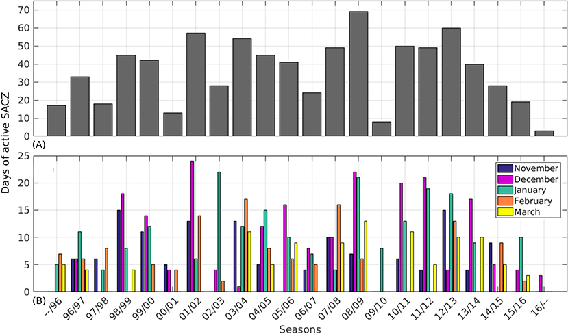
Figure 4. SACZ occurrence as detected by the automated method in days. (A) Days of SACZ occurrence per 5-months season (NDJFM) and per month in (B).
The agreement between the visual and automated number of SACZ reinforces the importance of using a temporal criterion. Carvalho et al. (2002) considered every day with convective adjacent pixels crossing the SACZ coastal region in the DJF months from 1979 to 1996. The authors found a total of 1,576 SACZ active days leading to a monthly average of ≈ 26 SACZ active days, an overestimation of 288% compared to the visual SACZ observations from CPTEC-INPE.
The SACZ differs from a frontal system specially due to the non-transient character. To lose the characteristics of a stationary front (e.g., temperature contrast between the air masses) and to acquire the SACZ dynamic features, the system must remain motionless for a few days. The observational study from Quadro (1994) concluded that a minimum of 4 consecutive days is sufficient to the frontal system acquire the SACZ dynamic characteristics, which was corroborated by Siqueira and Toledo Machado (2004) and Ambrizzi and Ferraz (2015).
Figures 4A,B shows the automated SACZ days over the 21 austral summers considered. The reduction in the number of active SACZ days after December of 2013 coincides with the beginning of a severe drought, mostly over São Paulo state, that lasted until 2015 (Coelho et al., 2016a,b). This is in agreement with the below average number of active SACZ in the 2014–2015 and 2015–2016 summers in Figures 4A,B. The above mentioned drought was a consequence of a tropic-extra tropic atmospheric teleconnection, where a positive SST anomaly over the Southwest Pacific results in a barotropic high over the Southwest Atlantic ocean after a few days, via Rossby waves propagation, blocking the passage of frontal systems and the SACZ formation (Grimm and Silva Dias, 1995; Coelho et al., 2016b).
In the next paragraphs we analyzed four austral summers in which the number of automated SACZ stayed below and above the seasonal average in Figure 4.
The 2000/2001 and 2009/2010 summers were marked by below mean SACZ active days (13 and 8, respectively). In the summer of 2000/2001 de Moraes Drumond and Ambrizzi (2005) observed a low-level anomalous anticyclonic circulation positioned over eastern Brazil, which inhibited the SACZ formation. The SACZ formation was also inhibited in the 2009/2010 summer, except by the occurrence of the Upper Tropospheric Cyclonic Vortice (UTCV) over South America in all summer months (http://climanalise.cptec.inpe.br/~rclimanl/boletim/index1209.shtml).
During 2008/2009 and 2012/2013, on the other hand, there were above average SACZ active days (69 and 60, respectively). This is consistent with visual observations of SACZ from CPTEC-INPE, with 69 visual SACZ days in 2008/2009 summer and 67 in 2012/2013. It is also consistent with the above historical mean precipitation under the SACZ regions in most of the summer months in 2008/2009 and 2013/2013; http://climanalise.cptec.inpe.br/~rclimanl/boletim/index1209.shtml). The 2013 summer season will be further explored in section 4.3.
The present objective methodology is simple and based on OLR only. Despite that, the hit rate of the algorithm was 77% (Table 1) and only 13% of the automated SACZ days disagree with the visual ones (Figure 2). Considering the above seasonal analysis and that the visual classifications are always subject to human interpretation, as exposed in section 2, we considered that the algorithm method satisfactorily represents the SACZ occurrence.
4.2. SACZ Climatology
Figure 5 shows the composites of SACZ active days for the OLR (left panels) and divergence of water vapor flux (right panel) fields. In Figures 5A,B it is possible to see that the SACZ signal occurred approximately in the same position for automated and visual SACZ. The Brazilian states locations are indicated in Figure 5A. The NW-SE orientation is evident extending from the Amazon to the SWAT and crossing the Brazilian coastline over the states of Espírito Santo (ES), Rio de Janeiro (RJ), and São Paulo (SP), between 18 and 27°S. This is in agreement with Kodama (1992), Ferreira et al. (2004) and for some episodes of SACZ found by Carvalho et al. (2002) and Jorgetti et al. (2014). The SACZ convection is maintained by the low level convergence of water vapor flux (Figures 5D,E), with maximum convergence over the Amazon forest and minimum over the oceanic SACZ portion. The difference between these two regions is of one order of magnitude. The topography of the east coast of Brazil is characterized by the presence of mountain chains that rises to an altitude of 500–1,000 m. The topography forces the ascendant motion of the air mass coming from the Amazon basin windward of the mountains, causing water vapor condensation. In Figures 5D,E the orographic effect is evident along the Brazilian east coast, with maximum (minimum) convergence of water vapor flux windward (leeward) of it.
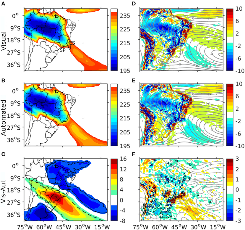
Figure 5. Composites of active SACZ days of (A,B) OLR (W m−2) and (D,E) divergence of water vapor flux (colors in × 108 s−1) and streamlines in 850 hPa. (C,F) Are the difference between visual (A,D) and automated (B,E) methods with significant t-test values (>95%) inside the solid and dashed lines.
The convergence of water vapor flux and streamlines pattern in Figures 5D,E indicate that water vapor comes to the SACZ region from the evaporation of the Tropical Atlantic Ocean surface (positive values around 10°S/30°W in Figures 5D,E), through the trade winds. This is consistent with the evaporation rate over the Atlantic ocean and vertically integrated moisture flux shown in Figures 20 and 21 of Kodama (1992). This is also in agreement with de Oliveira Vieira et al. (2013), which demonstrated that during SACZ active phase the lower-tropospheric transport of moisture increases in the northern boundary of the south Amazon Basin, reaching a 5 mm day−1 precipitation rate due to the moisture convergence. The divergence of water vapor flux associated with streamlines direction over northern Argentina, Uruguay and southern Brazil, a region known as Southeastern South America (SESA), indicate that this is another possible source of water vapor to the SACZ coastal and oceanic SACZ portions. However, the amount of water vapor that is transported to the SACZ was not calculated in the present work.
On average the automated SACZ is more intense over the coastal and oceanic SACZ regions and slightly displaced southwestward compared to visual SACZ (Figure 5C). The 850 hPa circulation pattern is the same for both automated and visual SACZ (Figure 5). However, it is important to notice in Figures 5E,F the intensification of the low pressure atmospheric system called Chaco Low (20°S/60°W), the compensatory high pressure system located south of it (36°S/65°W) and the trough near the Uruguay coast (36°/45°W) in the automated SACZ composite.
In Figure 6 the composite of the daily mean precipitation for the active SACZ is shown for visual (A) and automated (B) SACZ. The intensification of the dynamic circulation during the automated SACZ is accompanied by an increase in the daily mean precipitation across the Brazilian Southeast of about 3 mm day−1 (negative values in Figure 6C). Grimm et al. (2007) and Kodama et al. (2012) argued that the release of latent heat associated with precipitation in the Brazilian Southeast and the orographic effect of the Brazilian east coast mountain chains helps to maintain the cyclonic low level circulation (Chaco Low) through the conditional instability of the second kind (CISK) mechanism. The Chaco Low intensification accompanied by more precipitation over it during the automated SACZ (Figures 5D,E, 6A,B) corroborates with the thermal maintenance of the Chacho Low proposed by Grimm et al. (2007) and Kodama et al. (2012).
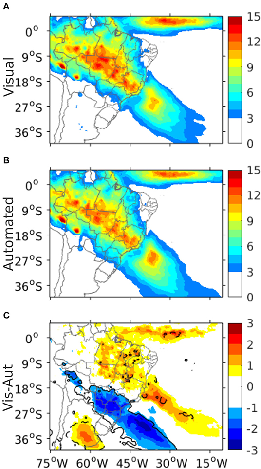
Figure 6. Composite of daily mean precipitation (mm day−1) for visual (A) and automated (B) SACZ active days and the difference between them (C) with significant t-test values (>95%) inside the solid and dashed lines.
The atmospheric dynamics contributes to anchoring the SACZ in its climatological position, mainly in the SACZ coastal and oceanic portions, through the ascending movement ahead of the semi stationary mid-tropospheric trough (Figures 7A,B). Figures 7A,B shows subsident movement over the SESA region, confirmed by Figures 6A,B, that shows a daily mean precipitation of ≈ 15 mm day−1 underneath the SACZ cloud band and <3 mm day−1 in SESA. This is also in agreement with several works that described the inhibition of precipitation in SESA during the days of active SACZ (Nógues-Peagle and Mo, 1997; Barros et al., 2000; Bombardi et al., 2014).
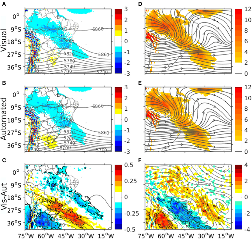
Figure 7. As in Figure 5, but for (A,B) omega velocity (colors in hPa s−1) and geopotential height (lines with intervals of 20 m) in 500 hPa and (D,E) divergence of mass (colors in × 106 s−1) and streamlines in 200 hPa. (C,F) Are the difference between visual (A,D) and automated (B,E) methods with significant t-test values (> 95%) inside the solid and dashed lines.
The subsidence over the SESA during a period of increased latent heat released in the Amazon basin and in the SACZ region can be explained in terms of Rossby and mixed Rossby-gravity waves dispersion (Silva Dias et al., 1983; Gandu and Silva Dias, 1998). As the forcing (source of heat) becomes bigger, away from the Equator and greater in size (similar to the one showed in Figure 6), the slow atmospheric propagating modes (Rossby and mixed Rossby-gravity waves) are favored, intensifying the regional response to the heating (Silva Dias et al., 1983).
In the upper troposphere at 200 hPa there is intensification and displacement to the west of the semi stationary trough axis (near the Uruguay coast) and of the ridge in the SACZ region during the automated SACZ days (Figures 7D–F). The 500 hPa ascending movement and the 200 hPa mass divergence are more intense and shifted to the southwest in the algorithm method, which is more evident over the SWAT (colors in Figures 7C,F).
Many of the South America summer upper tropospheric circulation features are connected to heat sources in the lower troposphere through a dynamical response to the heating (Kousky and Alonso Gan, 1981; Silva Dias et al., 1983; Gandu and Silva Dias, 1998). Heating through Amazon basin and SACZ coastal region displace the Bolivian High to southeast, intensifies the northeastern Brazilian trough and intensifies and displace the trough near the Uruguay coast to southwest in the upper troposphere (Gandu and Silva Dias, 1998). That is basically the SACZ configuration shown in Figures 7D,E.
The main difference between active and inactive SACZ days in the South America upper tropospheric circulation is the presence of the barotropic trough near the Uruguay coast in the former situation, while the Brazilian Northeastern Low and the Bolivian High are present in both cases (figures not shown). Moreover, during the No-SACZ days the mid-tropospheric ascendant movement (at 500 hPa) and the mass divergence (at 200 hPa) occur only over the continent, i.e., the SACZ oceanic portion vanishes. In the lower troposphere, at 850 hPa, the Chaco Low and the Uruguayan trough vanishes, the flow turns to the South of Brazil due to the west displacement of the South Atlantic Subtropical High (SASH) and a region of convergence of water vapor flux is found over the SWAT, but spatially separated from the continent during the No-SACZ days. In summary, the convective activity does not extend to the Southwestern Atlantic Ocean and there is no trough near the Uruguay coast during the No-SACZ days. The difference between active and inactive SACZ days is statistically significant according to the t-Student test with confidence level of 95% (figures not shown).
Therefore, the barotropic trough near the Uruguay coast is the key dynamic feature responsible for maintain a link between the SACZ continental and oceanic regions, because it contributes to support the convergence of water vapor flux and the consequent upward movement and precipitation in these regions. This trough also seems to define the intensity of the SACZ, with stronger trough (automated SACZ) associated with more intense SACZ in its coastal and oceanic regions (Figures 5C, 6C, 7C), which is in agreement with several previous works (Grimm and Silva Dias, 1995; Carvalho et al., 2002; Siqueira and Toledo Machado, 2004; Cunningham and Cavalcanti, 2006; Jorgetti et al., 2014).
The mean characteristics of the automated SACZ are described in Table 3. The average permanence of a SACZ episode is 6 days, varying from 4, as imposed by the algorithm, to 17 days. The values in Table 3 refer to the pixels within the CSG(n) that were classified as SACZ days. The total area covered by the SACZ convective activity (continental plus oceanic) is ~9.2 millions km2, while the area over the ocean is 2.6 millions km2, about 30% of the total size.
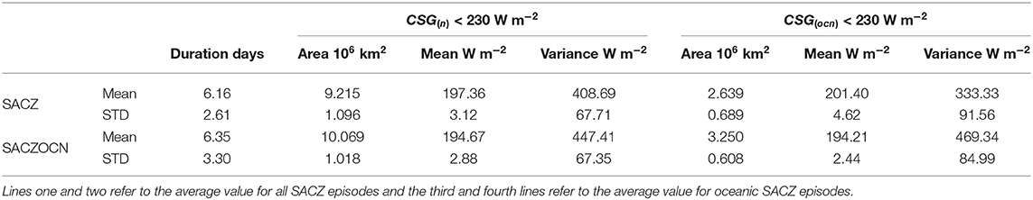
Table 3. Characteristics of the SACZ based on the CSG(n) and CSG(ocn) properties.
The average OLR within the CSG(n) is 197 W m−2 and 201 W m−2 for the pixels of the CSG(n) over the ocean, with standard deviations of 3.12 and 4.62 W m−2, respectively. The OLR variance is 408 W m−2 for the pixels inside the CSG(n) and 333 W m−2 for the pixels of the CSG(n) over the ocean, as showed in Table 3. The lower the OLR the more intense the convection, while the variance of the OLR pixels is proportionally related to the convection intensity in the SACZ region (Carvalho et al., 2002). Lower values of OLR and higher values of variance through the total SACZ area are associated with strong convection in the Amazon basin.
As discussed above, the oceanic SACZ portion is distinct from the continental one, and is related to the intensity of the convection in southeastern Brazil. In the next section we explore the characteristics of an oceanic SACZ episode.
4.3. Oceanic SACZ Climatology
In the present study, oceanic SACZ (SACZOCN) episodes are those in which the convective activity over the ocean is strong. Consider that j is a SACZ episode and varies from j = 1, 2, …, J, where J is the total number of SACZ episodes. CSG(ocn,j) is the spatial and temporal mean of the OLR pixels inside the CSG(n) that occurred over the ocean during the j SACZ episode. Remember that a SACZ episode lasts ~6 days (Table 3). CSG(ocn,J) is the spatial and temporal mean of the OLR pixels inside the CSG(n) that occurred over the ocean during the J SACZ episodes. The j SACZ episode is considered as SACZOCN episode if the CSG(ocn,j) is at least one standard deviation lower than the CSG(ocn,J), as follows:
Where std is the standard deviation. We found 108 SACZOCN days divided into 17 SACZOCN episodes. The SACZOCN episodes are highlighted in light gray in Table S2 and their average characteristics are shown in the last two lines of Table 3. The SACZOCN persistence is also ~6 days and the main differences comparing to SACZ are in the intensity and size of the episodes. The average OLR over the ocean during SACZOCN episodes is 194.21 W m−2, 7.2 W m−2 smaller than during SACZ episodes. The SACZOCN area over the ocean is 3.25 millions km2, 1.475 millions km2 greater than during SACZ episodes. In summary, SACZOCN episodes are more convective and bigger over the oceanic SACZ portion (Table 3).
During SACZOCN episodes there is a significant intensification and northward shift of the convective band, as can be seen in Figure 8B. The moisture divergence (Figures 8C,D) follows the same pattern, with increased convergence below the low values of OLR. The climatological position of the SACZOCN is over RJ, ES and south of Bahia states (i.e., more precipitation shifted to the north).
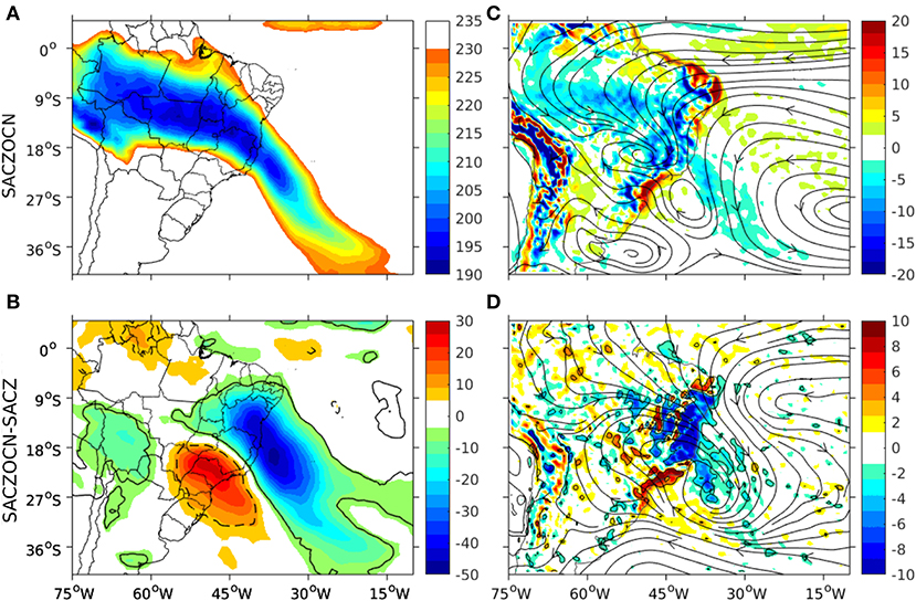
Figure 8. Composites for oceanic SACZ (SACZOCN) days. (A) OLR (W m−2). (C) divergence of water vapor flux (colors in × 108 s−1) and streamlines in 850 hPa. (B,D) are the difference between continental (SACZ) and SACZOCN, with significant t-test values (>95%) inside the solid and dashed lines.
A striking SACZOCN episode occurred from 10 to 26 of December, 2013. This episode was primarily responsible for one of the worst floods registered in the ES state (Matos et al., 2014). Also, in December of 2013, below historical mean precipitation occurred in the SP state, south of ES (http://climanalise.cptec.inpe.br/rclimanl/boletim/index1213.shtml), associated with the northward shift of the SACZOCN cloud band showed in Figure 8. Therefore, knowing when these events occurred can help to understand their origins and improve its predictability.
During SACZOCN episodes the trough near Uruguay coast closes into a cyclonic vortex and moves northward, near the southeast coast of Brazil (compare Figure 4D with Figure 8C). Brasiliense et al. (2018) named this closed cyclonic circulation as cyclonic vortex embedded in the SACZ (CVES). From Figures 8A,C it is clear that the CVES is not embedded in the SACZ, but southwest of it, near the RJ coast (see the location of RJ in Figure 5A). Thereby, a better name to the CVES could be cyclonic vortex southwest of the SACZ (CVSS). The SACZ is characterized by a trough near the Uruguay coast (Figures 5D,E), while the SACZOCN is characterized by the CVSS near southeastern Brazil (Figure 8C). Therefore, the CVSS can be used as the dynamic feature that characterizes the oceanic SACZ.
It is worth mentioning that one possible explanation for the northward shift of the SACZOCN is found in Cunningham and Cavalcanti (2006). The authors suggested that the northward displacement is correlated with the active phase of the zonal convective propagating pattern called Madden-Jullian Oscillation (MJO). The mechanism proposed is that large-scale convection over the Indonesia region can advect high potential vorticity air equatorward and induce ascending movement in the SPCZ, favoring its formation (Matthews et al., 1996; Cunningham and Cavalcanti, 2006). From Grimm and Silva Dias (1995) it is known that the SPCZ activity is able to trigger a SACZ episode after a few days—because the convection over the SPCZ results in anomalous upper tropospheric divergence in the SACZ region, which generates the trough near the Uruguay coast. To investigate if our SACZOCN episodes are related to the MJO further analyses have to be done.
Figure 9 shows the main variables that play a role on ocean-atmosphere interactions (e.g., surface currents, SST, incident daytime shortwave radiation, and 10 m wind) during the SACZOCN, inactive SACZ and the difference between them. The 10 m wind pattern is similar to that at 850 hPa (Figure 8), with a clear reversal in the wind direction through the Brazilian coast during the SACZOCN (Figures 9D,E). The difference in the wind speed during SACZOCN and No-SACZ days reaches 3 m s−1. Changes in the surface oceanic currents are only apparent in the difference panel (Figure 9C), where the same 10 m wind pattern is observed. The incident daytime shortwave radiation and the SST under the SACZOCN cloud band are, respectively, 200 W m−2 and 1.5 °C lower than in the No-SACZ. However, it is important to notice that the oceanic cooling extends eastward off the SACZOCN cloud band in the latitude belt 15–30°S.
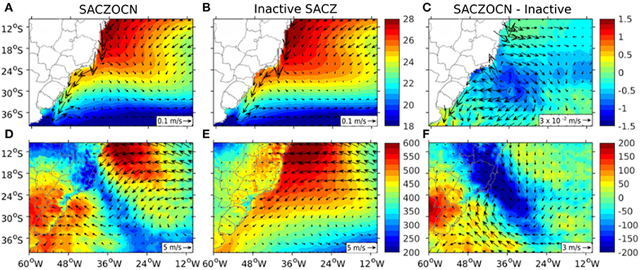
Figure 9. (A,B) SST (°C) and superficial oceanic currents (m s−1). (D,E) daily time downward shortwave radiation (W m−2) and 10 m wind. (A,D) are the composites for the SACZOCN episodes and (B,E) are the composites for inactive SACZ days. (C,F) are the difference between SACZOCN and inactive SACZ.
Figure 9C indicates that SACZOCN can induce changes in the oceanic surface currents in three main regions: (i) Cabo Frio, where the north to south surface flow tends to be weaker; (ii) the south coast of the Bahia state (18°S) and ES with intensification of the eastward surface flow and (iii) the open Subtropical Atlantic just off the southeast coast of Brazil, where the CVSS can induce the Ekman pumping.
Some authors had already suggested a dynamic mechanism for the cooling of the ocean surface during SACZ episodes (Kalnay et al., 1986; Chaves and Nobre, 2004; De Almeida et al., 2007), but none of them showed explicitly the ocean surface currents.
5. Summary and Conclusions
In the present work we proposed a simplified and objective method to detect SACZ episodes based on satellite OLR data classification. Different combinations for the threshold values in the algorithm were tested against visual SACZ classification. Visual classifications are always subjected to interpreter considerations and therefore must be treated carefully. However, visual SACZ dates were only available dates for comparison. The advantage of an automated method is that the classification process is not dependent on subjective interpretation, and therefore is reproducible.
The algorithm agreed with visual SACZ classification in 77% of the times. However, 13% of the automated SACZ days were not observed (false positive days). The temporal criterion of permanency of the SACZ convective activity for at least 4 days was essential to differentiate the SACZ from the transient frontal systems that pass over the Brazilian Southeast. We suggest for future works that the proposed method can be combined with that developed by Ambrizzi and Ferraz (2015), in order to improve the SACZ automated detection.
The period of active SACZ was 7.5 (8.9) days per month and 37.7 (44.6) days per 5-months season for the automated (visual) method. Also, ~30% of the SACZ active days occurred in November and March and 70% during the DJF trimester. For future SACZ studies we highlight the importance of: (i) considering only active SACZ days instead of the monthly average and (ii) include the months of November and March to fully represent the SACZ activity.
Automated and visual methodologies showed the same SACZ atmospheric pattern. The main dynamic structures present are: (i) low-level cyclonic circulation over the continent (Chaco Low closed or not); (ii) barotropic trough near the Uruguayan coast; (iii) a trough off the Northeast Brazilian coast in the upper troposphere and (iv) the Bolivian High also in the upper troposphere. All these dynamic features are in agreement with several works about SACZ activity (Kodama, 1992; Quadro, 1994; Ferreira et al., 2004), showing that our methodology is efficient in detecting the SACZ occurrence. Our results indicate that the intensity and position of the barotropic trough near the Uruguayan coast influences the intensity and position of the coastal and oceanic SACZ convective activity.
Oceanic SACZ episodes were objectively identified for the first time in the literature. The SACZOCN is characterized by the closing and northward shift of the Uruguayan trough, which we called cyclonic vortex southwest of SACZ (CVSS). The two main consequences of CVSS presence are that the convective activity associated with the SACZ becomes more intense and occurs north of the climatological position. We suggest that the CVSS can be used as a practical criterion to distinguish the SACZ and the SACZOCN.
SACZOCN episodes are able to modify the oceanic surface currents through the Brazilian coastline and underneath the CVSS. This is a strong evidence that the oceanic vertical velocity field can be modified by SACZOCN via Ekman transport on the coastal region and Ekman pumping in the open ocean. Besides, the decreasing SST underneath the SACZOCN cloud band compared to No-SACZ days reinforces the thermodynamic effect of this atmospheric system over the ocean.
Finally, we consider that our method is an useful tool for SACZ and SACZOCN detection, given the correct representation of both and the high agreement (77%) with the visual SACZ detection method. Besides, the ability to distinguish SACZ and SACZOCN is an advantage when compared to existing methods. We also highlight the possibility of implementing the algorithm in operational centers and its applicability in future climate scenarios.
Data Availability Statement
Publicly available datasets were analyzed in this study. This data can be found here: http://climanalise.cptec.inpe.br/rclimanl/boletim/, https://rda.ucar.edu/, https://www.ncdc.noaa.gov/cdr/atmospheric/outgoing-longwave-radiation-daily, http://www.gloh2o.org/.
Author Contributions
ER developed the proposed methodology with theoretical support of LP and MQ. NB led the English review. All authors contributed to the discussion and helped in writing the manuscript.
Funding
This study was financed in part by the Coordenação de Aperfeiçoamento de Pessoal de Nível Superior—Brasil (CAPES)—Finance Code 001. The authors also thank the funding support from CAPES in the project Advanced Studies in Oceanography of Medium and High Latitudes (CAPES 23038.004304/2014-28). This was also a contribution to ATMOS Project (CNPq 443013/2018-7). CNPq also funds LP through fellowship of the Research Productivity Program (CNPq 304009/2016-4).
Conflict of Interest
The authors declare that the research was conducted in the absence of any commercial or financial relationships that could be construed as a potential conflict of interest.
Acknowledgments
We acknowledge Dr. Pedro Silva Dias and Dr. João Antonio Lorenzzetti for great suggestions during the method development. The three reviewers provided comments which reflected substantial improvements to this paper and we are grateful for that.
Supplementary Material
The Supplementary Material for this article can be found online at: https://www.frontiersin.org/articles/10.3389/fenvs.2020.00018/full#supplementary-material
References
Ambrizzi, T., and Ferraz, S. E. (2015). An objective criterion for determining the south atlantic convergence zone. Front. Environ. Sci. 3:23. doi: 10.3389/fenvs.2015.00023
Barros, V., Gonzalez, M., Liebmann, B., and Camilloni, I. (2000). Influence of the South Atlantic Convergence Zone and the South Atlantic sea surface temperature on interannual summer rainfall variability in southeastern south america. Theor. Appl. Climatol. 67, 123–133. doi: 10.1007/s007040070002
Beck, H. E., Wood, E. F., Pan, M., Fisher, C. K., Miralles, D. G., Van Dijk, A. I., et al. (2019). Mswep v2 global 3-hourly 0.1° precipitation: methodology and quantitative assessment. Bull. Am. Meteorol. Soc. 100, 473–500. doi: 10.1175/BAMS-D-17-0138.1
Bombardi, R. J., Carvalho, L. M., Jones, C., and Reboita, M. S. (2014). Precipitation over Eastern South America and the South Atlantic Sea surface temperature during neutral ENSO periods. Clim. Dyn. 42, 1553–1568. doi: 10.1007/s00382-013-1832-7
Brasiliense, C. S., Dereczynski, C. P., Satyamurty, P., Chou, S. C., da Silva Santos, V. R., and Calado, R. N. (2018). Synoptic analysis of an intense rainfall event in Paraíba do Sul river basin in southeast Brazil. Meteorol. Appl. 25, 66–77. doi: 10.1002/met.1670
Carvalho, L. M. V., Jones, C., and Liebmann, B. (2002). Extreme precipitation events in Southeastern South America and large–scale convective patterns in the South Atlantic Convergence Zone. J. Clim. 15, 2377–2394. doi: 10.1175/1520-0442(2002)015<2377:EPEISS>2.0.CO;2
Chaves, R. R., and Nobre, P. (2004). Interactions between sea surface temperature over the South Atlantic Ocean and the South Atlantic Convergence Zone. Geophys. Res. Lett. 31:L03204. doi: 10.1029/2003GL018647
Coelho, C. A., Cardoso, D. H., and Firpo, M. A. (2016a). Precipitation diagnostics of an exceptionally dry event in São Paulo, Brazil. Theor. Appl. Climatol. 125, 769–784. doi: 10.1007/s00704-015-1540-9
Coelho, C. A., de Oliveira, C. P., Ambrizzi, T., Reboita, M. S., Carpenedo, C. B., Campos, J. L. P. S., et al. (2016b). The 2014 southeast brazil austral summer drought: regional scale mechanisms and teleconnections. Clim. Dyn. 46, 3737–3752. doi: 10.1007/s00382-015-2800-1
Cunningham, C. A. C., and Cavalcanti, I. F. A. (2006). Intraseasonal modes of variability affecting the South Atlantic Convergence Zone. Int. J. Climatol. 26, 1165–1180. doi: 10.1002/joc.1309
De Almeida, R. A. F., Nobre, P., Haarsma, R., and Campos, E. (2007). Negative ocean-atmosphere feedback in the South Atlantic convergence zone. Geophys. Res. Lett. 34:L18809. doi: 10.1029/2007GL030401
de Moraes Drumond, A. R., and Ambrizzi, T. (2005). The role of SST on the South American atmospheric circulation during January, February and March 2001. Clim. Dyn. 24, 781–791. doi: 10.1007/s00382-004-0472-3
de Oliveira Vieira, S., Satyamurty, P., and Andreoli, R. V. (2013). On the South Atlantic Convergence Zone affecting southern Amazonia in Austral summer. Atmos. Sci. Lett. 14, 1–6. doi: 10.1002/asl2.401
Fawcett, T. (2005). An introduction to ROC analysis. Pattern Recogn. Lett. 27, 861–874. doi: 10.1016/j.patrec.2005.10.010
Ferreira, N., Sanches, M., and Dias, M. A. F. S. (2004). Composite analysis of the South Atlantic Convergence Zone during el Niño and la Niña periods. Rev. Brasil. Meteorol. 19, 89–98.
Figueroa, S. N., Satyamurty, P., and Da Silva Dias, P. L. (1995). Simulations of the summer circulation over the South American region with an ETA coordinate model. J. Atmos. Sci. 52, 1573–1584.
Gan, M., Kousky, V., and Ropelewski, C. (2004). The South America monsoon circulation and its relationship to rainfall over west-central Brazil. J. Clim. 17, 47–66. doi: 10.1175/1520-0442(2004)017<0047:TSAMCA>2.0.CO;2
Gandu, A. W., and Silva Dias, P. L. (1998). Impact of tropical heat sources on the South American tropospheric upper circulation and subsidence. J. Geophys. Res. Atmos. 103, 6001–6015. doi: 10.1029/97JD03114
Grimm, A. M., Pal, J. S., and Giorgi, F. (2007). Connection between spring conditions and peak summer monsoon rainfall in South America: role of soil moisture, surface temperature, and topography in eastern Brazil. J. Clim. 20, 5929–5945. doi: 10.1175/2007JCLI1684.1
Grimm, A. M., and Silva Dias, P. L. (1995). Analysis of tropical-extratropical interactions with influence functions of a barotropic model. J. Atmos. Sci. 52, 3538–3555.
Houze, R. A. Jr. (2004). Mesoscale convective systems. Rev. Geophys. 42, 1–43. doi: 10.1029/2004RG000150
Jorgetti, T., Dias, P. L. S., and Freitas, E. D. (2014). The relationship between South Atlantic SST and SACZ intensity and positioning. Clim. Dyn. 42, 3077–3086. doi: 10.1007/s00382-013-1998-z
Kalnay, E., Mo, K. C., and Peagle, J. (1986). Large-amplitude, short-scale stationary rossby waves in the southern hemisphere: observations and mechanistic experiments to determine their origin. Am. Meteorol. Soc. 43, 252–275. doi: 10.1175/1520-0469(1986)043<0252:LASSSR>2.0.CO;2
Kasahara, A., and Silva Dias, P. L. (1986). Response of planetary waves to stationary tropical heating in a global atmosphere with meridional and vertical shear. J. Atmos. Sci. 43, 1893–1912.
Kiladis, G. N., and Weickmann, K. M. (1992). Circulation anomalies associated with tropical convection during northern winter. Monthly Weather Rev. 120, 1900–1923.
Kiladis, G. N., and Weickmann, K. M. (1997). Horizontal structure and seasonality of large-scale circulations associated with submonthly tropical convection. Monthly Weather Rev. 125, 1997–2013.
Kodama, Y. (1992). Large-scale common features of subtropical precipitation zones (the Baiu frontal zone, the SPCZ, and the SACZ) part I: Characteristics of subtropical frontal zones. J. Meteorol. Soc. Japan 70, 813–836.
Kodama, Y. (1993). Large-scale common features of subtropical precipitation zones (the Baiu frontal zone, the SPCZ, and the SACZ) part II: Conditions of the circulations for generating the stczs. J. Meteorol. Soc. Japan 71, 581–610.
Kodama, Y., Sagawa, T., Ishida, S., and Yoshikane, T. (2012). Roles of the Brazilian plateau in the formation of the SACZ. J. Clim. 25, 1745–1758. doi: 10.1175/2011JCLI3785.1
Kodama, Y.-M. (1999). Roles of the atmospheric heat sources in maintaining the subtropical convergence zones: an aqua-planet GCM study. J. Atmos. Sci. 56, 4032–4049.
Kousky, V. E., and Alonso Gan, M. (1981). Upper tropospheric cyclonic vortices in the tropical South Atlantic. Tellus 33, 538–551.
Lee, H.-T., Heidinger, A., Gruber, A., and Ellingson, G. R. (2004). The HIRs outgoing longwave radiation product from hybrid polar and geosynchronous satellite observations. Adv. Space Res. 33, 1120–1124. doi: 10.1016/S0273-1177(03)00750-6
Liebmann, B., Kiladis, G. N., Marengo, J. A., Ambrizzi, T., and Glick, J. D. (1999). Submonthly convective variability over South America and the South Atlantic Convergence Zone. J. Clim. 12, 1877–1891.
Marengo, J. A., Liebmann, B., Kousky, V. E., Filizola, N. P., and Wainer, I. C. (2001). Onset and end of the rainy season in the Brazilian Amazon basin. J. Clim. 14, 833–852. doi: 10.1175/1520-0442(2001)014<0833:OAEOTR>2.0.CO;2
Matos, A. J. S., Silva, A. S., Almeida, I. S., and Candido, M. O. (2014). “Assessment of a real-time flood forecasting at the Doce river basin: summer 2013 event,” in 6th International Conference on Flood Management (São Paulo: Brazilian Association of Water Resources–ABRHidro). Available online at: http://eventos.abrh.org.br/icfm6/proceedings/ (accessed February 2, 2020).
Matthews, A. J., Hoskins, B. J., Slingo, J. M., and Blackburn, M. (1996). Development of convection along the spcz within a Madden-Julian oscillation. Q. J. R. Meteorol. Soc. 122, 669–688.
Nógues-Peagle, J., and Mo, K. C. (1997). Alternating wet and dry conditions over south america during summer. Monthly Weather Rev. 125, 279–291.
Quadro, M. F. L. (1994). Cases study of the South Atlantic Convergence Zone (SACZ) over the South America (Master's thesis), National Institute for Spatial Research [INPE-6341-TDI/593].
Rao, V., and Hada, K. (1990). Characteristics of rainfall over Brazil: annual variations and connections with the southern oscillation. Theor. Appl. Climatol. 42, 81–91.
Romatschke, U., and Houze, R. A. Jr. (2010). Extreme summer convection in South America. J. Clim. 23, 3761–3791. doi: 10.1175/2010JCLI3465.1
Romatschke, U., and Houze, R. A. Jr. (2013). Characteristics of precipitating convective systems accounting for the summer rainfall of tropical and subtropical South America. J. Hydrometeorol. 14, 25–46. doi: 10.1175/JHM-D-12-060.1
Rosso, F. V., Boiaski, N. T., Ferraz, S. E. T., and Robles, T. C. (2018). Influence of the Antarctic oscillation on the South Atlantic Convergence Zone. Atmosphere 9:431. doi: 10.3390/atmos9110431
Saha, S., Moorthi, S., Pan, H.-L., Wu, X., Wang, J., Nadiga, S., et al. (2010). NCEP Climate Forecast System Reanalysis (CFSR) 6-Hourly Products, January 1979 to December 2010. Boulder, CO: Research Data Archive at the National Center for Atmospheric Research, Computational and Information Systems Laboratory.
Saha, S., Moorthi, S., Wu, X., Wang, J., Nadiga, S., Tripp, P., et al. (2011). NCEP Climate Forecast System Version 2 (CFSV2) 6-Hourly Products. Boulder, CO: Research Data Archive at the National Center for Atmospheric Research, Computational and Information Systems Laboratory.
Satyamurty, P., and De Mattos, L. F. (1989). Climatological lower tropospheric frontogenesis in the midlatitudes due to horizontal deformation and divergence. Monthly Weather Rev. 117, 1355–1364.
Satyamurty, P., and Rosa, M. B. (2019). Synoptic climatology of tropical and subtropical South America and adjoining seas as inferred from geostationary operational environmental satellite imagery. Int. J. Climatol. 40, 378–399. doi: 10.1002/joc.6217
Seo, H., Jochum, M., Murtugudde, R., Miller, A. J., and Roads, J. O. (2008). Precipitation from African easterly waves in a coupled model of the tropical Atlantic. J. Clim. 21, 1417–1431. doi: 10.1175/2007JCLI1906.1
Silva Dias, P. L., Schubert, W. H., and DeMaria, M. (1983). Large-scale response of the tropical atmosphere to transient convection. J. Atmos. Sci. 40, 2689–2707.
Siqueira, J. R., and Toledo Machado, L. A. (2004). Influence of the frontal systems on the day-to-day convection variability over South America. J. Clim. 17, 1754–1766. doi: 10.1175/1520-0442(2004)017<1754:IOTFSO>2.0.CO;2
Streten, N. A. (1973). Some characteristics of satellite-observed bands of persistent cloudiness over the southern hemisphere. Monthly Weather Rev. 101, 486–495.
Taljaard, J. J. (1972). “Synoptic meteorology of the southern hemisphere,” in Meteorology of the Southern Hemisphere, Volume XIII of Meteorological Monographs. 1st Edn., ed C. W. Newton (Boston, MA: American Meteorological Society), 139–211.
Virji, H. (1981). A preliminary study of summertime tropospheric circulation patterns over south america estimated from cloud winds. Monthly Weather Rev. 109, 599–610.
Wilks, D. (1995). Statistical Methods in the Atmospheric Sciences: An Introduction, Vol. 59 of International Geophysics Series. San Diego, CA: Academic Press.
Yassunary, T. (1977). Stationary waves in the southern hemisphere mid-latitude zonal revealed from averages brightness charts. J. Meteorol. Soc. Japan 55, 274–285.
Keywords: South Atlantic Convergence Zone, oceanic SACZ, climatology, automated method, algorithm, OLR
Citation: Rosa EB, Pezzi LP, Quadro MFLd and Brunsell N (2020) Automated Detection Algorithm for SACZ, Oceanic SACZ, and Their Climatological Features. Front. Environ. Sci. 8:18. doi: 10.3389/fenvs.2020.00018
Received: 15 August 2019; Accepted: 05 February 2020;
Published: 25 February 2020.
Edited by:
Alexandre M. Ramos, University of Lisbon, PortugalReviewed by:
Jorge Eiras-Barca, University of Illinois at Urbana-Champaign, United StatesLuana Albertani Pampuch, São Paulo State University, Brazil
Prakki Satyamurty, National Institute of Amazonian Research (INPA), Brazil
Copyright © 2020 Rosa, Pezzi, Quadro and Brunsell. This is an open-access article distributed under the terms of the Creative Commons Attribution License (CC BY). The use, distribution or reproduction in other forums is permitted, provided the original author(s) and the copyright owner(s) are credited and that the original publication in this journal is cited, in accordance with accepted academic practice. No use, distribution or reproduction is permitted which does not comply with these terms.
*Correspondence: Eliana Bertol Rosa, eliana.rosa@inpe.br; elianaocn@gmail.com