A Comparison of Three Different Methods for the Identification of Hysterically Degrading Structures Using BWBN Model

Zhao, Ying; Noori, Mohammad; Altabey, Wael A.; Awad, Taher

doi:10.3389/fbuil.2018.00080

ORIGINAL RESEARCH article

Front. Built Environ., 07 January 2019
Sec. Computational Methods in Structural Engineering
Volume 4 - 2018 | https://doi.org/10.3389/fbuil.2018.00080

A Comparison of Three Different Methods for the Identification of Hysterically Degrading Structures Using BWBN Model

Ying Zhao¹

Mohammad Noori^1,2^*

Wael A. Altabey^1,3,4

Taher Awad⁴

¹International Institute for Urban Systems Engineering, Southeast University, Nanjing, China
²Department of Mechanical Engineering, California Polytechnic State University, San Luis Obispo, CA, United States
³Nanjing Zhixing Information Technology Company, Nanjing, China
⁴Department of Mechanical Engineering, Faculty of Engineering, Alexandria University, Alexandria, Egypt

Structural control and health monitoring scheme play key roles not only in enhancing the safety and reliability of infrastructure systems when they are subjected to natural disasters, such as earthquakes, high winds, and sea waves, but it also optimally minimize the life cycle cost and maximize the whole performance through the full life cycle design. In this scheme, system identification is regarded as a major technique to identify system states and related parameter variables, thus preventing degradation of structural or mechanical systems when unexpected disturbances occur. In this paper, three different strategies are proposed to identify general hysteretic behavior of a typical shear structure subjected to external excitations. Different case studies are presented to analyze the dynamic responses of a time varying shear structural system with the early version of Bouc-Wen-Baber-Noori (BWBN) hysteresis model. By incorporating a “Gray Box” strategy utilizing an Intelligent Parameter Varying (IPV) and Artificial Neural Network (ANN) approach, a Genetic algorithm (GA), and a Transitional Markov Chain Monte Carlo (TMCMC) based Bayesian Updating framework system identification schemes are developed to identify the hysteretic behavior of the structural system. Hysteresis characteristics, computational accuracy, and algorithm efficiency are further discussed by evaluating the system identification results. Results show that IPV performs superior computational efficiency and system identification accuracy over GA and TMCMC approaches.

Introduction

In recent years, an increasing attention is witnessed to face the challenging issues of safety, serviceability, reliability, risk and life-cycle management, and performance improvement of structures and infrastructure due to changing and more frequently occurring natural and man-made hazards, infrastructure crisis, and sustainability issues. These disturbances are dealt with innovative technologies to enhance structural functionality and safety in various stages of research and development (Spencer, 2003; Altabey, 2017a). Several types of structures that employ control strategies for different application scopes can be found in Constantinou et al. (1998), Soong and Spencer (2002), and Altabey (2014, 2017b,c); Altabey (2018). Proper modeling of inherent non-linearity in vast majority of structural systems plays an important role in understanding structural response under hazardous loadings. System identification is an important approach in control strategy regarded as the interface between the mathematical world of control theory and the real world of application and model abstractions (Zadeh, 1956; Ljung, 2010; Altabey, 2016, 2017d,e; Altabey and Noori, 2017a, 2018; Zhao et al., 2018), and it handles a wide range of system dynamics problem without the prior knowledge of actual system physics. The schematic diagram of system identification process is depicted in Figure 1.

FIGURE 1

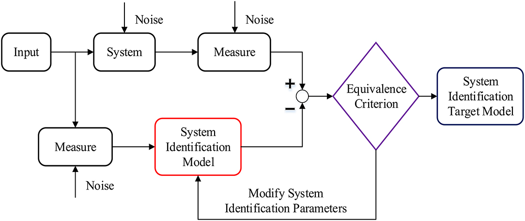
Figure 1. A diagram of system identification.

Hysteresis can be described as the hereditary and memory nature of a non-linear or inelastic system behavior where the restoring force is dependent on both instantaneous as well as past history of deformations. In general, under cyclic loading, mechanical and structural systems are capable of dissipating considerable energy and they exhibit appreciable hysteretic behavior with hysteresis loops. Each loop enclosing the area in the restoring force vs. displacement curve depicts the energy dissipated over a complete cycle resulting from internal friction within the structural system.

Various empirical hysteresis models have been proposed in the past few decades. A class of smoothly varying hysteresis models used in engineering fields are Bouc-Wen class of hysteresis models. Bouc suggested a smooth and versatile hysteresis model for non-linear systems and hysteretic systems (Bouc, 1967; Wen, 1975, 1976, 1980, 1986, 1989; Park et al., 1986; Wen and Yeh, 1989; Ikhouane and Rodellar, 2007; Ikhouane et al., 2007; Ikhouane and Gomis-Bellmunt, 2008). Baber and Wen extended the Bouc model to take the degradation in strength or stiffness of structural systems into account (Baber and Wen, 1980). Baber-Noori, and later Noori, further extended the capabilities of Bouc-Wen model by including pinching behavior and studied the response of these systems under random excitation (Noori, 1984; Baber and Noori, 1986). Baber-Noori and subsequently Noori-Baber's work on integrating the pinching phenomenon in hysteretic behavior and extending Bouc-Wen-Baber (BWB) model was the first work in developing a smooth hysteresis model capable of taking into account strength and stiffness degradation as well as shear pinching phenomenon (Baber and Noori, 1985). BWBN was incorporated in structural design software, OpenSees developed at the University of California Berkeley (Hossain, 1995). A toolbox for computing the parameters of BWBN hysteresis model using multi-objective optimization evolutionary algorithms was also developed by SourceForge, an Open Source community (Bouc Wen Baber Noori Model of Hysteresis, Source Forge). Foliente showed Bouc-Wen-Baber-Noori (BWBN) model could produce previously observed inelastic behavior of wood joints and structural systems using BWBN smooth hysteresis model (Foliente, 1995; Zhao et al., 2017a,b; Noori et al., 2018). Deb et al. developed a toolbox that identifies structural parameters of Bouc–Wen–Baber–Noori hysteresis model through a noval multi-objective optimization evolutionary algorithms (MOBEAs) (Deb et al., 2002; Deb, 2013). Ortiz et al. analyzed and identified BWBN model via a multi-objective optimization algorithm (Ortiz et al., 2013). Peng et al. utilized BWBN model for identifying the parameters of a magneto-rheological damper and depicts its force-lag phenomenon (Peng et al., 2014). Muller et al. investigated the application of BWBN in their work and conducted performance-based seismic design through a Search-Based Cost Optimization (Muller et al., 2012). Chan et al. made a prediction of the hysteretic behavior of passive control systems by applying BWBN in a nonlinear-autoregressive-exogenous model (Chan et al., 2015).

Traditional artificial neural networks technique shows its superiority in the identification, monitoring, and control of complicated and non-linear dynamic systems (Narendra and Parthasarathy, 1990; Masri et al., 1992; Lu and Basar, 1998; Abouelwafa et al., 2014; Altabey and Noori, 2017b). However, a priori knowledge of the characteristics of restoring force is necessary and important for traditional parametric system identification approaches, while the non-parametric methods do not need information beforehand, lacking direct association between system dynamics and system model. In order to overcome the limitations of conventional parametric and non-parametric approaches, an noval Intelligent Parameter Varying (IPV) method was proposed, which makes full use of the embedded radial basis function networks to make an estimation of the hysteretic and inelastic characteristics of restoring forces constitutively for a multi degree of freedom system. A scaled three story base excited structure was designed to experimentally verify the non-linearity and its associated hysteresis of a structure using a displacement controlled shaking table (Saadat et al., 2003, 2004a,b, 2007). Further, a data-driven identification strategy for non-linear and hysteretic behaviors of steel wire strands was compared and verified using polynomial basis functions and neural networks. The results showed that neural networks were found more promising for the prediction of slightly pinched, hardening hysteresis, strongly pinched, hardening hysteresis, and classical quasi-linear softening hysteresis (Brewick et al., 2016). Genetic algorithms have been used for system identification of non-linear and hysteretic systems. The application of Real Coded Genetic Algorithms (RCGA) was demonstrated and applied to fit curves of synthetic and experimentally obtained Bouc-Wen hysteresis loops for a sandwich composite material (Hornig and Flowers, 2005). Different real coded genetic algorithms and their related criteria for efficiently identifying non-linear systems are regards as non-classical and optimized identification techniques (Monti et al., 2009). A Bayesian probabilistic framework was proposed to detect damage of continuous monitored structures by incorporating load-dependent Ritz vectors as an alternative to modal vectors (Sohn, 1998). A large body of work was conducted to track, estimate and identify structural parameters, system status and hysteretic and degrading behavior of structures using Kalman filters, extended Kalman filters and unscented Kalman filters (Jeen-Shang and Yigong, 1994; Yang et al., 2006; Wu and Smyth, 2007, 2008; Chatzi and Smyth, 2009; Chatzi et al., 2010; Lei and Jiang, 2011; Mu et al., 2013; Kontoroupi and Smyth, 2017; Erazo and Nagarajaiah, 2018). Traditional Markov Chain Monte Carlo approach in conjunction with Bayesian updating method were applied for structural response predictions and performance reliability evaluation (Yuen and Katafygiotis, 2001; Zhang and Cho, 2001; Beck and Au, 2002). Later, a transitional Markov Chain Monte Carlo (TMCMC) approach was developed by designing optimized sampling strategy from a series of intermediate probability density functions (PDFs) that converge to the target PDF, thus avoiding sampling difficulties. The TMCMC theory and algorithm were verified and demonstrated through the performance of the developed sampling approach, different PDFs as well as higher dimensional problems (Ching and Chen, 2007; Muto, 2007; Muto and Beck, 2008; Worden and Hensman, 2012; Zheng and Yu, 2013; Behmanesh and Moaveni, 2014; Green, 2015; Green et al., 2015; Ortiz et al., 2015).

It is a major barrier to successfully design hysteretic structures against degradation under severe cyclic loading. Most structural systems degrade with significant hysteresis, for example wood structures, dams, highways, reinforced concrete towers, steel bridges are critical and key elements of our built environment. In spite of their obvious importance, and their huge rehabilitation and replacement costs, design, construction, and analysis of the majority of these structures requires overly simplistic or in some cases flawed assumptions regarding hysteretic evolution. Development of a practical structural degrading identification approaches is much deserving. A comparative study of online and offline identification strategies for UAVs were discussed, and it is found that online approach is more adaptive to changes but with lower prediction accuracy (Puttige and Anavatti, 2007). Therefore, offline learning is employed in this paper. Based on what was discussed in the introduction above, the main contributions of the research are to present a three story hysteretically degrading shear structure by incorporating BWBN slip lock hysteresis to represent the hysteretic restoring forces in this system. This BWBN model will be capable of producing all significant and prominent features of structural strength and stiffness degradations as well as slip lock behavior, and conduct a comparative study using three system identification approaches including an Intelligent Parameter Varying Artificial Neural Network developed in an earlier research work by a group that involved one of the authors (a “gray box” model that considers linear as well as non-linear parts of the dynamic system), genetic algorithm optimization method, and a novel TMCMC statistical approach.

The comparative study of the aforementioned approaches for system identification and their application in a structural system using BWBN MODEL is an original work. To the best of the authors' knowledge such comparative study has not been reported in the literature.

Structural System Modeling and System Identification

BWBN Hysteresis Model

The model employed herein is an earlier version of BWBN hysteresis degradation model, which incorporates the previous smooth system degrading element by Bouc as modified by Baber and Wen in series with a slip-lock element (a non-linear hardening spring) developed by Baber and Noori. Under cyclic excitation, degradation manifests itself in the evolution of progressively varying hysteresis loops. A non-linear system governed by Equation (1) is given with the incorporation of BWBN model.

\begin{matrix} m \ddot{x} + c \dot{x} + R = F (t) & (1) \end{matrix}

\begin{matrix} R = α k x + (1 - α) k z & (2) \end{matrix}

\begin{matrix} \dot{z} = \frac{A {\dot{x}}_{1} - ν [β | {\dot{x}}_{1} | | z |^{n - 1} z + γ {\dot{x}}_{1} | z |^{n}]}{η} & (3) \end{matrix}

\begin{matrix} {\dot{x}}_{2} = \sqrt{\frac{2}{π}} \frac{s}{σ} \exp [- \frac{z^{2}}{2 σ^{2}}] \dot{z} & (4) \end{matrix}

\begin{matrix} \dot{ε} = (1 - α) k \dot{x} z & (5) \end{matrix}

\begin{matrix} s = δ_{s} ε & (6) \end{matrix}

\begin{matrix} (x = x_{1} + x_{2}) & (7) \end{matrix}

where, parameters m, c, k are, respectively, the mass, damping, and stiffness coefficients, and parameters ẍ, ẋ, x are quantities that describe the system acceleration, velocity and displacement, and R is the restoring force and F(t) is the ambient excitation. Parameter α is the weighting value denoting the ratio of post-elastic to initial stiffness. Parameters A, β, and γ are basic hysteresis shape control parameters. Parameter z is the hysteretic displacement, and n is the degree of the sharpness of yield. Strength and stiffness degradation coefficients are, respectively denoted by ν(δ_ν) and η(δ_η). Parameters x₁ and x₂ are Bouc-Wen hysteretic system displacement and the additional displacement that considers slip-lock behavior. Parameter ε is the measure of the combined effect of duration and severity of the energy dissipated through hysteresis, σ is a measure of the sharpness of the peak of the hysteresis, and δ_s measures the slip magnitude. All 10 parameters are essential to produce the common features of hysteretic behavior. It would be very helpful if a small number of unspecified parameters for system identification can be reduced in that large numbers of parameters increase the uncertainty of convergence for updating parameters in search space. It was proved that the redundancy of specific hysteresis parameters can be eliminated through mathematical transformations in the parameter space devised to freeze them without affecting the system response (Ma et al., 2004; Charalampakis and Koumousis, 2008a,b; Charalampakis and Dimou, 2010).

Structural System Modeling

Restoring force curves of reinforced or steel structures show complex hysteresis characteristics, revealing material non-linearity, crack opening and closing, bond and slip between steel bars and concrete and low cycle fatigue that result in structural strength and stiffness degradation. The hysteresis model used herein considers the specific case appropriate for both strength and stiffness degradations, and slip-lock behavior of restoring hysteretic forces of the structure. All the restoring forces of the structure are assumed to follow the BWBN hysteresis model. The structural system considered in this study is a shear type model subjected to ambient sinusoidal wave and ElCentro seismic excitation as input signals ẍ_g. The ground excitation motion ẍ_g makes an integral transformation to be incorporated into the structural equations. The structural system mainly includes three lumped mass coupled subsystems, as shown in Figure 2. These masses are lumped at floor (floor m_i), levels and these floors are assumed and constrained to only move laterally. The restoring force R_i , in conjunction with the stiffness between the adjacent floors, are represented by dampers and springs, with the corresponding coefficients c_i and k_i, respectively. The time varying system yields energy dissipation due to the hysteretic behavior of the inner structure.

FIGURE 2

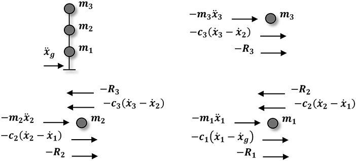
Figure 2. Structural lumped mass model.

For this three story shear structure, the equations of motion are represented by Equations (8–10):

\begin{matrix} m_{3} {\ddot{x}}_{3} + c_{3} ({\dot{x}}_{3} - {\dot{x}}_{2}) + R_{3} = 0 & (8) \end{matrix}

\begin{matrix} m_{2} {\ddot{x}}_{2} + c_{2} ({\dot{x}}_{2} - {\dot{x}}_{1}) + R_{2} - c_{3} ({\dot{x}}_{3} - {\dot{x}}_{2}) - R_{3} = 0 & (9) \end{matrix}

\begin{matrix} m_{1} {\ddot{x}}_{1} + c_{1} ({\dot{x}}_{1} - {\dot{x}}_{g}) + R_{1} - c_{2} ({\dot{x}}_{2} - {\dot{x}}_{1}) - R_{2} = 0 & (10) \end{matrix}

System Identification Theory

A typical system identification framework mainly has two components including system itself and system identification model. By defining an equivalence criterion, the parameters of the system identification model are updated via a comparison with the original system, until the system identification model will be eventually equivalent to the original system. System identification approaches used in this paper include intelligent parameter varying based approach, GA based approach and transitional markov chain monte carlo (TMCMC) based approach. IPV approach employs ANNs and establishes a “Gray Box” system, where the original system parameters are replaced by the parameters of ANNs, and the system structure is replaced by ANNs. For GA and TMCMC methods, they are used to optimize and identify the parameters of system model, which is regarded as an approximate model of the original real system. The theoretical background for the three approaches are presented in the following subsections.

Intelligent Parameter Varying Based System Identification

Artificial neural network (ANN) is a non-linear and adaptive information processing system composed of large numbers of neuron units. A radial basis function (RBF) neural network is employed to build the intelligent parameter varying model. In ANN architecture, the Euclidean distance between the clustering center and input vector is calculated and the result is activated to pass through the output layer. The activation function is Gaussian output function and is formulated as:

\begin{matrix} g_{j} = \exp (- \frac{\sum_{i = 1}^{n} {(x_{i} - c_{j})}^{2}}{σ_{j}^{2}}) & (11) \end{matrix}

where g_j is the output of the j^th unit in the hidden layer, x_i is the input data fed to the network, c_j is the center of the j^th unit in the input space, and σ_j is the width of the j^th function. j = 1, 2, ⋯ , m. Parameter m is the number of the centers of neurons, and n represents the dimension of the input space. Linearly weighted summation of hidden layer node outputs produces the output nodes. Therefore, the output of the network is calculated by:

\begin{matrix} y = \sum_{j = 1}^{n} w_{j} g_{j} & (12) \end{matrix}

where w_j is the weight of the j^th node.

The objective is to find a series of weights that minimize the square of error between the actual and desired network outputs, i.e.,:

\begin{matrix} E (k) = \frac{1}{2} \sum_{j = 1}^{N} {(d (k) - y (k))}^{2} & (13) \end{matrix}

where d(k) is the desired output and y(k) the actual output of RBF and j = 1, 2, ⋯ , N, and N is the number of data sets. There are commonly two approaches for utilizing ANNs, i.e., supervised and unsupervised learning. In supervised approach the input and the referred output are usually known. The network then processes the input values and makes a comparison between its resulting output and the desired output. The network system makes the errors propagate back through different layers, causing the system to adjust tuned weights which control the network. This process repeats over and over until all the weights are continually tweaked in an appropriate way. During the training process of a network the connection weights are continually refined to a specific generalization level and a good network performance level. In unsupervised training, the system itself must then decide what features and how many features need to be extracted to group the input data, which is often referred to as self-organization or adaption. Herein, we use the non-supervised learning algorithm to acquire the centers and variance of radial basis function, and meanwhile the least mean squared error is acquired by using supervised learning algorithm. The response of the hysteretic system is used as the desired signal, and the error between the desired signal and the simulated signal is back propagated to modify the weights and threshold values of neural network model.

Parametric system identification approaches have been widely used but in most published literature in this area a priori knowledge of the characteristics depicting the behavior of restoring force is required. Non-parametric approaches generally do not need information beforehand but they typically lack direct associations between system dynamics and associated model. When ANNs are implemented using the “Black Box” approach, little of the system information might be obtained from the traditional techniques due to the fact that the “Black Box” only considers system input and output. Intelligent Parameter Varying (IPV) method preserves the benefits of both traditional parametric and non-parametric approaches, and utilizes the embedded radial basis function as the activation of neurons to estimate the constitutive characteristics of inelastic and hysteretic restoring forces for a multi degree of freedom structural system.

IPV technique, i.e., a gray box approach (Figure 3) that incorporates the advantages of both “White Box” and “Black Box” approaches, was developed in such a way that the model structure can be determined using the first principle (Equations 18–20), while non-linear and adaptive learning capabilities of ANNs can be used to identify the non-linear, time varying system's dynamics (Equations 24–26) that would be difficult to model and identify using the traditional “White Box” and “Black Box” (Saadat et al., 2003, 2004a,b, 2007).

FIGURE 3

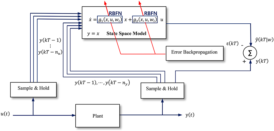
Figure 3. System identification using gray box.

A non-linear system with full state measurement represented by the Linear Parameter Varying (LPV) model structure is given by:

\begin{matrix} \dot{x} = f_{1} (x, u) \cdot x + f_{2} (x, u) \cdot u & (14) \end{matrix}

\begin{matrix} y = x & (15) \end{matrix}

The IPV approach introduced herein would preserve the model structure inherent in Equation (14) without requiring a priori representations of non-linearities f₁(x, u) and f₂(x, u). Instead, these terms would be represented by separate artificial neural networks g₁(x, u, w₁) and g₂(x, u, w₂) as depicted in Equations (16, 17):

\begin{matrix} \dot{x} = g_{1} (x, u, w_{1}) \cdot x + g_{2} (x, u, w_{2}) \cdot u & (16) \end{matrix}

\begin{matrix} y = x & (17) \end{matrix}

By modeling the non-linearities f₁(x, u) and f₂(x, u) via separate artificial neural networks g₁(x, u, w₁) and g₂(x, u, w₂), the model structure (Equations 16, 17) is preserved. Therefore, the relationship between the model structure and artificial neural network parameters is preserved. The structural model is preserved by incorporating ANN, preserving a portion of information of the structural model. The IPV approach preserves the direct association between the construction of ANN and the system dynamics, used for structural health monitoring for system identification.

Based on first principle, system dynamics can be transformed to the following form:

\begin{matrix} - c_{3} ({\dot{x}}_{3} - {\dot{x}}_{2}) - R_{3} - m_{3} {\ddot{x}}_{g} = m_{3} {\ddot{u}}_{3} & (18) \end{matrix}

\begin{matrix} - c_{2} ({\dot{x}}_{2} - {\dot{x}}_{1}) - R_{2} + c_{3} ({\dot{x}}_{3} - {\dot{x}}_{2}) + R_{3} - m_{2} {\ddot{x}}_{g} = m_{2} {\ddot{u}}_{2} & (19) \end{matrix}

\begin{matrix} - c_{1} ({\dot{x}}_{1} - {\dot{x}}_{g}) - R_{1} + c_{2} ({\dot{x}}_{2} - {\dot{x}}_{1}) + R_{2} - m_{1} {\ddot{x}}_{g} = m_{1} {\ddot{u}}_{1} & (20) \end{matrix}

where u₁, u₂, u₃, respectively represent the relative displacements of each floor, i.e., u₁ = x₁−x_g, u₂ = x₂−x_g, u₃ = x₃−x_g.

\begin{matrix} - R_{3} - m_{3} {\ddot{x}}_{g} = m_{3} ü_{3} & (21) \end{matrix}

\begin{matrix} - R_{2} + R_{3} - m_{2} {\ddot{x}}_{g} = m_{2} ü_{2} & (22) \end{matrix}

\begin{matrix} - R_{1} + R_{2} - m_{1} {\ddot{x}}_{g} = m_{1} ü_{1} & (23) \end{matrix}

The stiffness and damping terms are lumped into restoring forces, since in the hysteresis models the restoring force R associates with the lateral relative displacement x_r and the restoring displacement z, where z is expressed by the function of lateral relative velocity ẋ_r.

The modeling for the restoring forces using radial basis function based neural network is as follows:

\begin{matrix} {\hat{R}}_{3} = g_{3} (ü_{3}, {\ddot{x}}_{g}) & (24) \end{matrix}

\begin{matrix} {\hat{R}}_{2} = g_{2} (ü_{2}, {\ddot{x}}_{g}, {\hat{R}}_{3}) & (25) \end{matrix}

\begin{matrix} {\hat{R}}_{1} = g_{1} (ü_{1}, {\ddot{x}}_{g}, {\hat{R}}_{2}) & (26) \end{matrix}

where, ${\hat{R}}_{1}, {\hat{R}}_{2}, {\hat{R}}_{3}$ represent, respectively, the identified restoring forces through the training of ANN as shown in Figure 4.

FIGURE 4

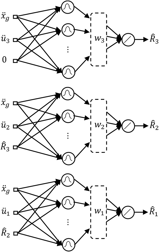
Figure 4. IPV for structural system modeling.

Genetic Algorithm Based System Identification

Genetic algorithm (GA) is an approach that searches the global optimal solution by simulating a natural evolution process. The objective function can be formulated as the normalized mean square error (MSE) of the predicted time history ỹ(t|p) as compared to the reference time history y(t). Herein, the acceleration response signal is employed as the time history series. The purpose of the following optimization approach is to minimize the difference (or the error) between predicted time history and the referred time history. The hysteretic structural system objective function is introduced below:

\begin{matrix} O F (p) = \frac{\sum_{i = 1}^{n} {(y (t_{i}) - \tilde{y} (t_{i} | p))}^{2}}{N σ_{y}^{2}} & (27) \end{matrix}

where p is a parameter vector, $σ_{y}^{2}$ the variance of the reference history, and N the number of points used. Sum of three acceleration response signal differences of the hysteretic structural system is used as the objective function. The optimization problem can be stated as the minimization of the objective function OF(p) when the parameter vector has the following side constraints as:

\begin{matrix} x_{L B} \leq p \leq x_{U B} & (28) \end{matrix}

where x_LB and x_UB are vectors defining the lower and the upper values of the model parameters, respectively. The basic strategy for the parameter identification using GA is shown in Figure 5. GA operates starting from a population of the potential solutions to a representive problem, and one population is composed of numbers of individuals coded by genes. Each individual is chromosomes with the characteristics of entity. GA initializes on a population of individuals (coded candidate solutions to the problem) that are manipulated by some operators such as selection, crossover, and mutation. In short, the selection process drives the search direction toward the region of best individuals, and the cross operator combines individuals to generate offsprings.

FIGURE 5

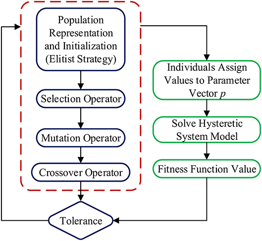
Figure 5. A flow chart of system identification using GA.

If it is indispensable to make selection and crossover operators converge toward the optimum, mutation alters one or more gene values (individuals) in a chromosome from its initial state, thus, maintaining genetic diversity from one generation of a population to the next. In this way, a complete exploration of global search space is forced by algorithm within the search space. Each individual in the population is represented as chromosome, indicating the collection of parameters are supposed to identify. GA adopts an elitist strategy, which consists of the preservation of the most fit individuals obtained in the current generation. Population representation and initialization generate population and individuals, and the initialized value will be assigned to the parameter space for solving the hysteretic system model. The fitness function is established by using the prediction error between the simulated signal response and predicted signal response. After a series of successive mathematical operators for optimization, the next generational loop begins.

Transitional Markov Chain Monte Carlo Based System Identification

Markov Chain Monte Carlo (MCMC) is an analytic approach which replaces numerical integration through summation over numbers of samples generated from iteration. A Markov chain is a stochastic process where one state is transformed to another state after a sufficiently long sequence of transition procedure. The next state is conditionally based on the last state. A key property of Markov chain is that the starting state has no influence on the state of the chain via a series of sequential transitions. The chain reaches its steady state at a specific point where it reflects sampling distribution from stationary status. The principle of Monte Carlo simulation is applied for the integration to approximate the expected complex distribution status of numbers of samples. By increasing the number of samples, the approximation accuracy can be measured and achieve a desired value, which mainly depends on the independence of the samples.

Markov chain involves a stochastic sequential process where a series of states can be sampled from some stationary distributions while Monte Carlo sampling can make an estimation of various characteristics of a specific distribution. The goal of MCMC is to design a Markov chain to meet the target distribution of the chain which is what we are interested in sampling from.

Transitional Markov Chain Monte Carlo Theory (TMCMC) is introduced to avoid the difficulty of sampling from complicated target probability distributions (e.g., multimodal PDFs, PDFs with flat manifold, and very peaked PDFs) but sampling from a series of intermediate PDFs that converge to the target PDF and are easier to sample.

Bayesian Inference describes a process of solving posterior density functions given the likelihood and prior probability. The target probabilistic model can be depicted by M, D is the data acquired from the system, and the uncertain parameters of the model are described as θ. Sampling from the posterior PDF of θ conditioned on D is the aim of the Baysian model updating, which is given as:

\begin{array}{l} \begin{matrix} f (θ | M, D) & = & \frac{f (D | M, θ) \cdot f (θ | M)}{f (D | M)} \end{matrix} \\ \begin{matrix} = & \frac{f (D | M, θ) \cdot f (θ | M)}{\int^{​} f (D | M, θ) \cdot f (θ | M) \cdot d θ} \end{matrix} & (29) \end{array}

where f(θ|M) is the prior PDF of θ, f(D|M, θ) is the likelihood of D given θ, and f(D|M) is the evidence of the model M.

Bayesian model updating generally employs simulation based methods in that it is effective to obtain samples from f(θ|M, θ), which can be estimated at a specific quantity of interest E(g|M, D) based on the Law of Large Number.

\begin{matrix} E (g | M, D) \approx \frac{1}{N} \sum_{k = 1}^{N} g (θ_{k}) & (30) \end{matrix}

where {θ_k:k = 1, 2, ⋯ , N} represents a set of N samples from f(θ|M, D). Consider the equation as follow:

\begin{matrix} f (θ | M, D) \propto f (θ | M) \cdot f (D | M, θ) & (31) \end{matrix}

It is usually difficult to sample from f(θ|M, D) using Importance Sampling (IS) and Metropolis–Hastings (MH) in that it is not so easy to understand the geometry of the likelihood f(D|M, θ). To converge to the target PDF f(θ|M, D) from the prior PDF f(θ|M), a series of intermediate PDFs are constructed as the following:

\begin{array}{l} \begin{matrix} f_{j} (θ) \propto f (θ | M) \cdot f {(D | M, θ)}^{p_{j}}, j = 0, 1, \dots, m \end{matrix} \\ \begin{matrix} 0 = p_{0} < p_{1} < \dots < p_{m} = 1 \end{matrix} & (32) \end{array}

Note that f₀(θ) = f(θ|M), f_m(θ) = f(θ|M, D).

where the index j denotes the stage number. Although the geometry changing from f(θ|M) to f(θ|M, D) is large, the status of two changing adjacent intermediate PDFs is small. It is efficient to sample from f_j+1(θ) according to the previous sample from f_j(θ) through this small change.

The function f_j(θ) is used to extract samples and make an estimation of the PDF itself as a kernel density function (KDF), a combination of weighted Gaussian functions centered at the samples. The kernel density function can be regarded as the proposal PDF of the MH method to sample from f_j+1(θ). This will subsequently and ultimately result in f(θ|M, D) samples. This approach is called adaptive Metropolis–Hastings (AMH) algorithm. Given that the proposal PDF (KDF) function is fixed, rendering the MH method is as similar as IS, not efficient in high dimension situation.

It is a totally different strategy for TMCMC to acquire f_j+1(θ) samples based on f_j(θ) samples, KDF method is replaced by a resampling algorithm. It covers a battery of resampling stages, with each stage completing the following, given N_j samples from f_j(θ), depicted by {θ_{j, k}:k = 1, ⋯ , N_j}, acquire samples from f_j+1(θ), depicted by{θ_{j+1, k}:k = 1, ⋯ , N_j+1}. It can be calculated by the following in a more easier way, with the samples {θ_{j, k}:k = 1, ⋯ , N_j} from f_j(θ). The “plausibility weights (w(θ_{j, k}))” of these samples regarding f_j+1(θ) can be computed by:

\begin{array}{l} \begin{matrix} w (θ_{j, k}) = \frac{f (θ_{j, k} | M) f {(D | M, θ_{j, k})}^{p_{j + 1}}}{f (θ_{j, k} | M) f {(D | M, θ_{j, k})}^{p_{j}}} & = & f {(D | M, θ_{j, k})}^{p_{j + 1} - p_{j}}, \end{matrix} \\ \begin{matrix} k & = & 1, \dots, N_{j} \end{matrix} & (33) \end{array}

Based on the normalized weights, the uncertain parameters can be resampled, i.e. let: θ_{j+1, k} = θ_{j, l} and $w . p . \frac{w (θ_{j, l})}{\sum_{l = 1}^{N_{j}} w (θ_{j, l})}$ k = 1, ⋯ , N_j+1

where “with probability” is represented by w.p. and pacifier index is denoted as l. It is shown that if N_j and N_j+1 achieve a relatively large quantity, {θ_{j+1, k}:k = 1, ⋯ , N_j+1} will be distributed as f_j+1(θ). Moreover, w(θ_{j, k}) is expected as the following value:

\begin{array}{l} E [w (θ_{j, k})] = \int^{​} w (θ) \cdot f_{j} (θ) \cdot d θ \\ = \int^{​} f {(D | M, θ)}^{p_{j + 1} - p_{j}} \cdot f_{j} (θ) \cdot d θ \\ = \int^{​} f {(D | M, θ)}^{p_{j + 1} - p_{j}} \cdot \frac{f (θ | M) f {(D | M, θ)}^{p_{j}}}{f (θ | M) f {(D | M, θ)}^{p_{j}} d θ} \cdot d θ \\ \begin{matrix} = & \frac{\int^{​} f (θ | M) f {(D | M, θ)}^{p_{j + 1}} d θ}{\int^{​} f (θ | M) f {(D | M, θ)}^{p_{j}} d θ} \end{matrix} & (34) \end{array}

Therefore, $\sum_{k = 1}^{N_{j}} w (θ_{j, k}) / N_{j}$ is the automatically unbiased estimation made for $\frac{\int {f (θ | M) f (D | M, θ)}^{p_{j + 1}} d θ}{\int {f (θ | M) f (D | M, θ)}^{p_{j}} d θ}$ . According to the results above, the following method is used to sample from f(θ|M, D) and make an estimation of f(D|M).

More precisely, with probability $w (θ_{j, k}) / \sum_{l = 1}^{N_{j}} w (θ_{j, l})$ , by using a covariance matrix equal to the scaled version of the estimated covariance matrix of f_j+1(θ), a Markov chain sample in the k^th chain can be generated from a Gaussian proposal PDF centered at the current sample of the k^th chain:

\begin{array}{l} \sum_{j}^{} = β^{2} \sum_{k = 1}^{N_{j}} w (θ_{j, k}) {θ_{j, k} - [\frac{\sum_{j = 1}^{N_{j}} w (θ_{j, l}) θ_{j, l}}{\sum_{j = 1}^{N_{j}} w (θ_{j, l})}]} \\ \times {θ_{j, k} - [\frac{\sum_{j = 1}^{N_{j}} w (θ_{j, l}) θ_{j, l}}{\sum_{j = 1}^{N_{j}} w (θ_{j, l})}]}^{T} & (35) \end{array}

where β is the prescribed scaling factor, $\sum_{j} = p r o d u c t o f β^{2}$ and the estimated covariance of f_j+1(θ). The rejection rate is chosen as the value β, and MCMC may probably achieve a larger value accordingly. The value 0.2 is found to be more reasonable for the scaling parameter β.

It is essential to choose {p_j:j = 1, ⋯ , m−1}. The larger value of p is desirable to make the transition between the intermediate adjacent PDFs smoother. The number of intermediate stages achieves a huge value if the increase of p-values has slow change rates.

The degree of uniformity of the plausibility weights {w(θ_{j, k}):k = 1, ⋯ , N_j} can appropriately indicate how close f_j+1(θ) approaches f_j(θ), so p_j+1 should be chosen so that the coefficient of variation (COV) of the plausibility weights can be equivalent to a prescribed threshold. The Bayesian inference framework for system identification is established (Figure 6) for structural model updating, which is regarded as a determinant reason for choosing the most suitable model parameters related to the hysteretic behavior of the structures by minimizing the difference between the predicted structural response and the simulated structural response. For the hysteretic structural model, the uncertain model parameters are selected as the ones that need to be updated through Bayesian inference (Equation 31) by drawing samples of parameters from the posterior PDF of parameters.

FIGURE 6

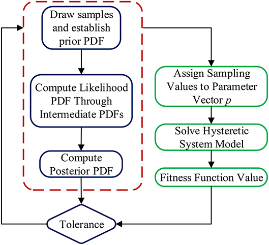
Figure 6. TMCMC based system identification strategy.

The TMCMC based Bayesian Updating algorithm is coded and implemented to establish the computational environment via exchange of data between the model and the algorithm. The evolution of parameter updating process is that, the samples from the prior PDFs are approximately uniformly distributed in the model parameter space at the first stage (p₀ = 0). Through applying Bayesian inference with TMCMC probabilistic simulations, the samples eventually populate well in the high probability region of the posterior PDFs close to the true model parameters at the last stage (p_m = 1).

TMCMC approach is employed to make an identification of the parameters of Bouc-Wen class models, henceforth represented by the vector θ ≤ Θ⊆R^d. The appropriate choice of θ reflects the corresponding non-linear and hysteretic behavior of structure. By applying Bayesian model updating, the major advantage is that the result gives a probability distribution expressing the likelihood probability distribution of different parameters rather than yielding a single value for θ. It is clear that the evolution of the model parameter variation represents the Bayesian inference process.

To make a restriction of the parameter space Θ, two side constraint vectors θ_min and θ_max are defined such that:

\begin{matrix} θ_{\min} (i) \leq θ (i) \leq θ_{\max} (i) 1 \leq i \leq d & (36) \end{matrix}

The vector θ has specific constraints such that the generated initial samples can determine the feasible values that the parameters can take. By defining prior PDF of θ a uniform distribution between the likelihood PDF and side constraints are regarded as the prediction error assumed as Gaussian function distributed with unknown variance and zero mean. The prediction error is described as the error between the predicted system response and the simulated system response given by:

\begin{matrix} f (D | θ) = \prod_{i = 1}^{l} \frac{1}{σ_{a c c} \sqrt{2 π}} \exp [- \frac{1}{2 σ_{a c c}^{2}} {(\frac{x (t_{i}) - \hat{x} (t_{i} | θ)}{S_{a c c} (t_{i})})}^{2}] & (37) \end{matrix}

where $σ_{a c c}^{2}$ is the variance of the prediction errors and S_acc is the weighting function used to normalize the acceleration response of the hysteretic system. To achieve computational convenience, the log-likelihood function lnf(D|θ) is employed in the actual implementation of the TMCMC algorithm as:

\begin{array}{l} \begin{matrix} l n f (D | θ) = & - & \frac{1}{2} N_{t} \ln (2 π) - N_{t} \ln (σ_{a c c}) \end{matrix} \\ \begin{matrix} - & \frac{1}{2 σ_{a c c}^{2}} {(\frac{x (t_{i}) - \hat{x} (t_{i} | θ)}{S_{a c c} (t_{i})})}^{2} \end{matrix} & (38) \end{array}

The j^th stage of parameter evolution process by correspondingly choosing the values of p_j can be shown as the contours of PDF f_j(θ).

Numerical Analysis of System Identification

Parameter Settings

Table 1 lists the parameter assignments of the structural system associated with BWBN hysteresis model for different cases. The mass coefficient of each floor is 1 kg, stiffness coefficient 10 N/m (sin) and 20 N/m (ElCentro), damping coefficient 0.05 N/(m/s) for each floor, respectively.

TABLE 1

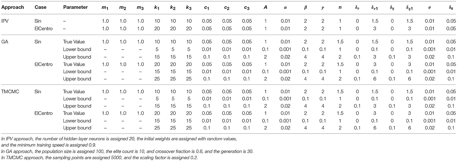
Table 1. Parameter assignment for different cases.

For hysteresis model, A = 1, α = 0.01, β = 2, γ = 2, n = 1 (IPV), n = 1.5 (GA and TMCMC), δ_ν = 0, δ_ν1 = 1.5 (sin) and 3 (ElCentro), δ_η = 0, δ_η1 = 1.5 (sin) and 3 (ElCentro), σ = 0.01, δ_s = 0.05. Damage occurrences are assumed at 30 s, 60 s, 100 s (sin) and 10 s, 20 s, 40 s (ElCentro) when both the strength degradation factor δ_υ and stiffness degradation factor δ_η change to δ_υ1and δ_η1, respectively. For GA and TMCMC approaches, parameter initial values are assigned between the corresponding lower and upper bounds before the optimization processes. Parameters are updated between the two bounds of parametric searching space, and eventurally achieve the exact values.

Numerical Analysis Results

Figures 7, 8 show the restoring force identification results when the structure is subjected to sinusoidal signal and ElCentro signal, respectively. Black curve represents the restoring force of the original structural system while the red curve represents the identified restoring force using IPV, GA, and TMCMC approaches. For the case of sinusoidal excitation, the identification results show that the degradation phenomenon of restoring forces of 2nd−3rd floor and 1st−2nd floor are more evident compared with ground-1st floor by using all of the three approaches. For the case of ElCentro excitation, the identification results show that the degradation phenomenon of restoring forces existing in all adjacent floors by using IPV and GA methods is more evident compared with that using TMCMC method. The hysteresis curves rotate accordingly when damage occurs. More results in details are discussed in the next section.

FIGURE 7

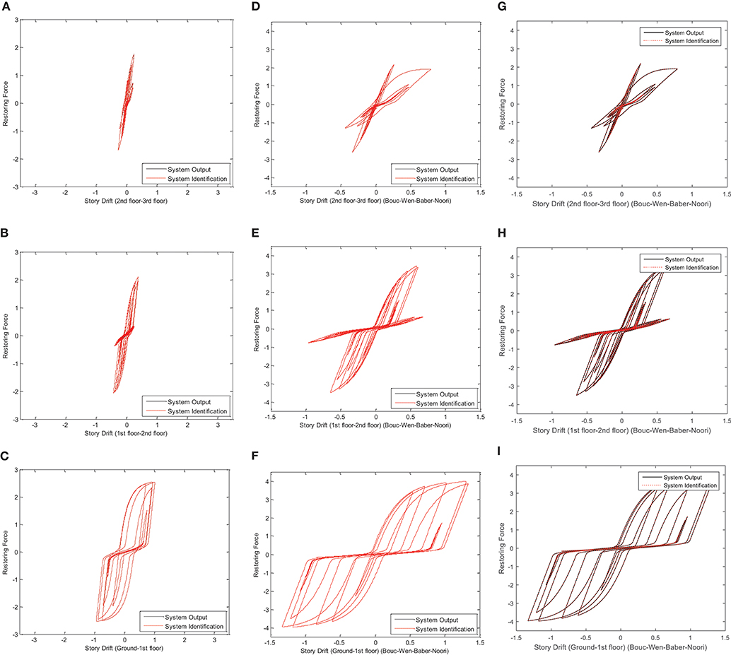
Figure 7. System identification results (Sin) (A–C) IPV, (D–F) GA, (G–I) TMCMC.

FIGURE 8

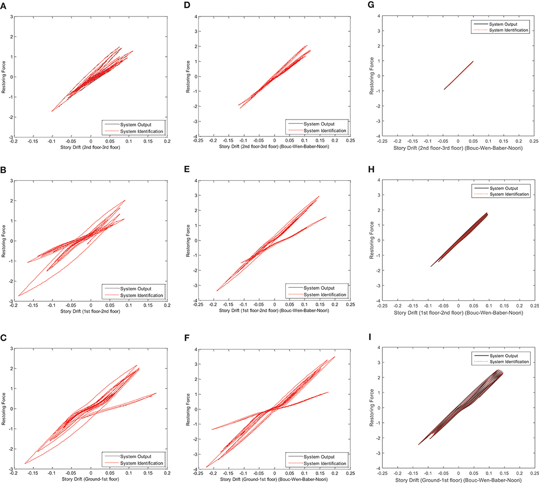
Figure 8. System identification results (ElCentro) (A–C) IPV, (D–F) GA, (G–I) TMCMC.

Discussions

Choice of Signal Excitation Type and Objective Function

Both sinusoidal excitation signal and ElCentro excitation signal are used as input signals to the system identification of hyestetic system. The frequency of sin signal is single and history curve is smooth and periodic variation. The ElCentro wave is stochastic, non-periodic, and non-steady state, and this represents the other type of excitation which is totally counter to harmonic wave such as sin signal. These two types of signals are employed to the response analysis and verification of the generalization capability of three different algorithms for identifying restoring forces of hysteretic structure. In addition, the establishment of objective functions employed in the GA and TMCMC are formulated through the combination of desired and simulated acceleration signal differences of all three degrees of freedom.

Parameter Choice for System Identification

Table 2 shows the parameter identification error using GA and TMCMC for the case of noise free, SNR = 30 and SNR = 10 (SNR = signal noise ratio). These error represents the relative error between the “true value” and “identified value.” All errors are no more than 10%. Generally for the cases with higher SNR they perform better parameter identification results since the disturbance of noise to signal is low. From Figures 7, 8, and Table 2, for the noise free case, it is shown that during the degradation process (damage evolution), strength degradation factor δ_υ changes from 0 to 1.4695 (sin,GA) /3.0130 (ElCentro,GA) /1.5913 (sin,TMCMC) /2.9890 (ElCentro,TMCMC), and stiffness degradation factor δ_η changes from 0 to 1.5370 (sin,GA)/2.9142 (ElCentro,GA)/1.5400 (sin,TMCMC)/2.7357 (ElCentro,TMCMC).

TABLE 2

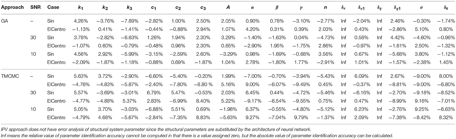
Table 2. Parameter identification error for different cases.

The hysteresis loop rotates clockwise with a certain degree, indicating large non-linearity and considerable degradation. However, from the identification results, it is also found that in the sin excitation case, the hysteresis loop exhibits better slip-lock phenomenon, and can absorb more energy than the case of ElCentro excitation. Noise corrupted cases have similar parameter identification results.

Table 3 shows the analysis of correlation coefficients for different cases. For the cases with small SNR, the identification effectiveness is not relatively good compared with noise free and higher SNR (R-t is the restoring force-time relationship, and R-x is the restoring force-relative displacement relationship).

TABLE 3

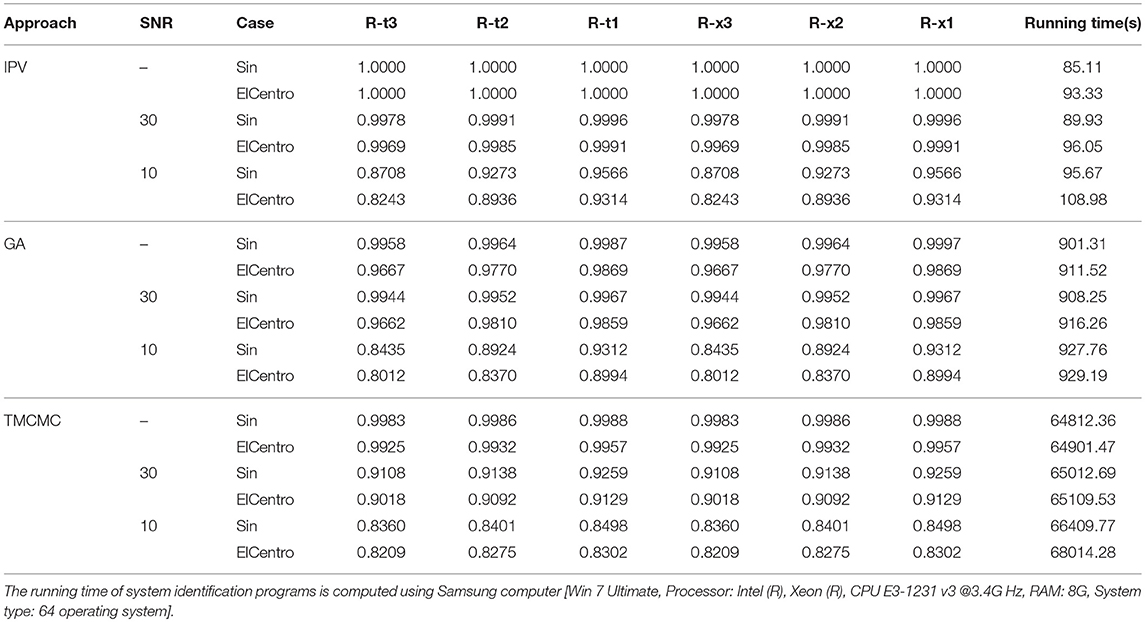
Table 3. Correlation coefficient analysis for different cases.

In this paper, IPV is a radius basis neural network which is a completely data-driven approach, while GA and TMCMC are not fully data-driven in that they assign the identification model within specific initial parameter intervals and then update and search to optimize structural model.

IPV method performs better identification results due to its adaptive learning capability and anti noise property in the noise environment. From computational time, it can be concluded that the IPV approach is a more efficient identification method compared with GA and TMCMC methods. Concretely, for the case of noise free, the computational time for GA and TMCMC are 9.59 and 760.51% longer than IPV (sin), and 8.77 and 694.40% longer than IPV (ElCentro). Similar results are also shown in noise corrupted cases. This demonstrates IPV method has higher computational efficiency than GA and TMCMC approaches.

Strength and stiffness degradation parameters are both very important in the hysteresis model, which determine the hysteretic behavior of structural systems. Table 4 lists five groups of parameter assignments regarding the variance of strength and stiffness degradation coefficients. The objective of setting these cases is studying the influence of change of degradation parameters on system identification accuracy.

TABLE 4

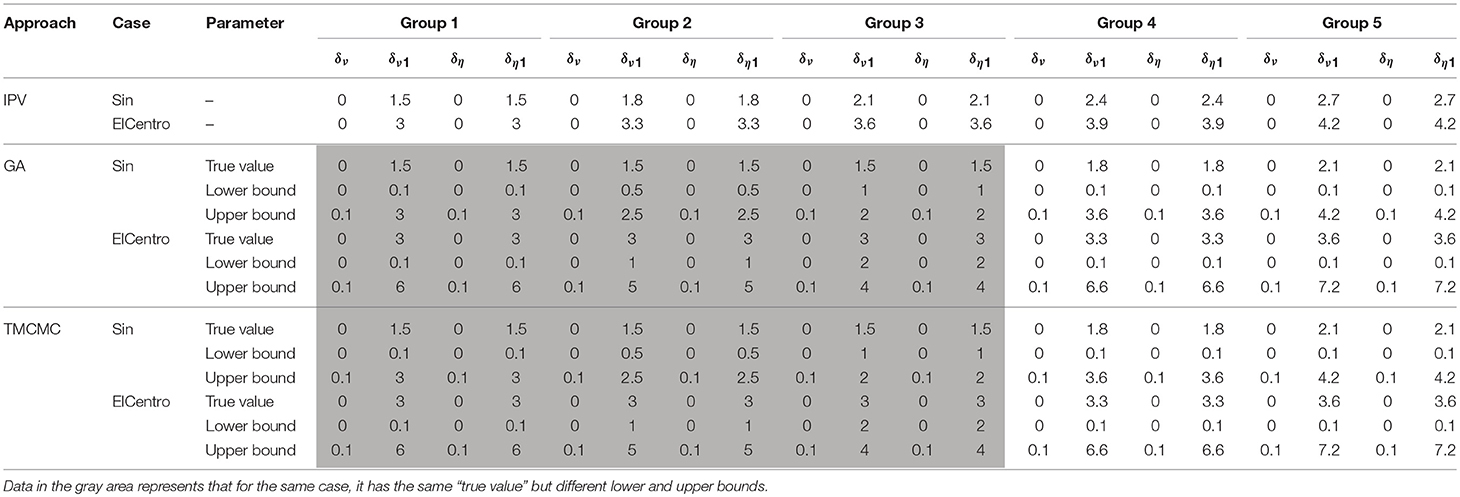
Table 4. Degradation parameter assignment for different cases.

To simulate damage occurrence, for IPV approach, strength degradation factor δ_υ and stiffness degradation factor δ_η change from 1.5 to 1.8, 2.1, 2.4, and 2.7, respectively (sin), while change from 3 to 3.3, 3.6, 3.9, and 4.2, respectively (ElCentro). For GA (sin) method, for the first three groups, the true value of strength degradation factor δ_υ and stiffness degradation factor δ_η keep fixed value 1.5 but the lower and upper bound change from 0.1–3 to 0.5–2.5 and 1–2, respectively. For the last two groups, the true value of strength degradation factor δ_υ and stiffness degradation factor δ_η are 1.8 and 2.1, respectively but the lower and upper bound correspondingly change from 0.1 to 3.6 and 0.1 to 4.2, respectively.

For GA (ElCentro) method, for the first three groups, the true value of strength degradation factor δ_υ and stiffness degradation factor δ_η keep fixed value 3 but the lower and upper bound change from 0.1–6 to 1–5 and 2–4, respectively. For the last two groups, the true value of strength degradation factor δ_υ and stiffness degradation factor δ_η are 3.3 and 3.6, respectively but the lower and upper bound correspondingly change from 0.1 to 6.6 and 0.1 to 7.2, respectively. TMCMC parameter assignment has similar cases.

Table 5 shows the influence of change of strength and stiffness degradation parameter on system identification accuracy indicated by correlation coefficients using IPV method. For sin excitation, as the strength and stiffness degradation parameter increase from 1.5 to 2.7, the correlation coefficients do not increase or decrease for the same case, and the computational time also keep almost unchanged: (sin) Group1: 85.11–95.67 s, Group 2: 89.01–104.78 s, Group 3: 88.97–107.37 s, Group 4: 83.12–100.20 s, Group 5: 86.09–104.55 s. (ElCentro) Group 1: 93.33–108.98 s, Group 2: 92.17–115.90 s, Group 3: 90.00–120.03 s, Group 4: 87.21–107.69 s, Group 5: 89.11–111.11 s.

TABLE 5

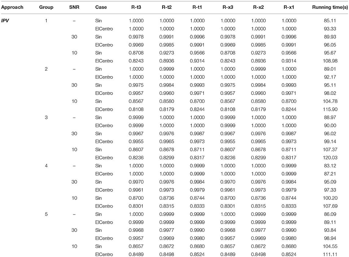
Table 5. Correlation coefficient analysis (IPV).

Table 6 shows the influence of change of strength and stiffness degradation parameter on system identification accuracy indicated by correlation coefficients using GA method. For sin excitation, when the strength and stiffness degradation parameter value is fixed at 1.5, as bounds (interval) change from 0–3 to 1–2, the correlation coefficients approach 1, indicating the system identification accuracy improves with the bound interval decreasing. The closer the bounds approach to the true value, the more accurate and deterministic the system identifiion results are. Accordingly, the computational time decreases with the bound interval decreasing. For details: Group 1: 901.31–927.76 s, Group 2: 895.66–922.22 s, Group 3: 889.73–914.73 s. When the true value of strength and stiffness degradation increases from 1.5 to 2.1 with given bounds, the identification accuracy decreases, and the computational time increases accordingly. Similar cases can also be found for ElCentro excitation signal.

TABLE 6

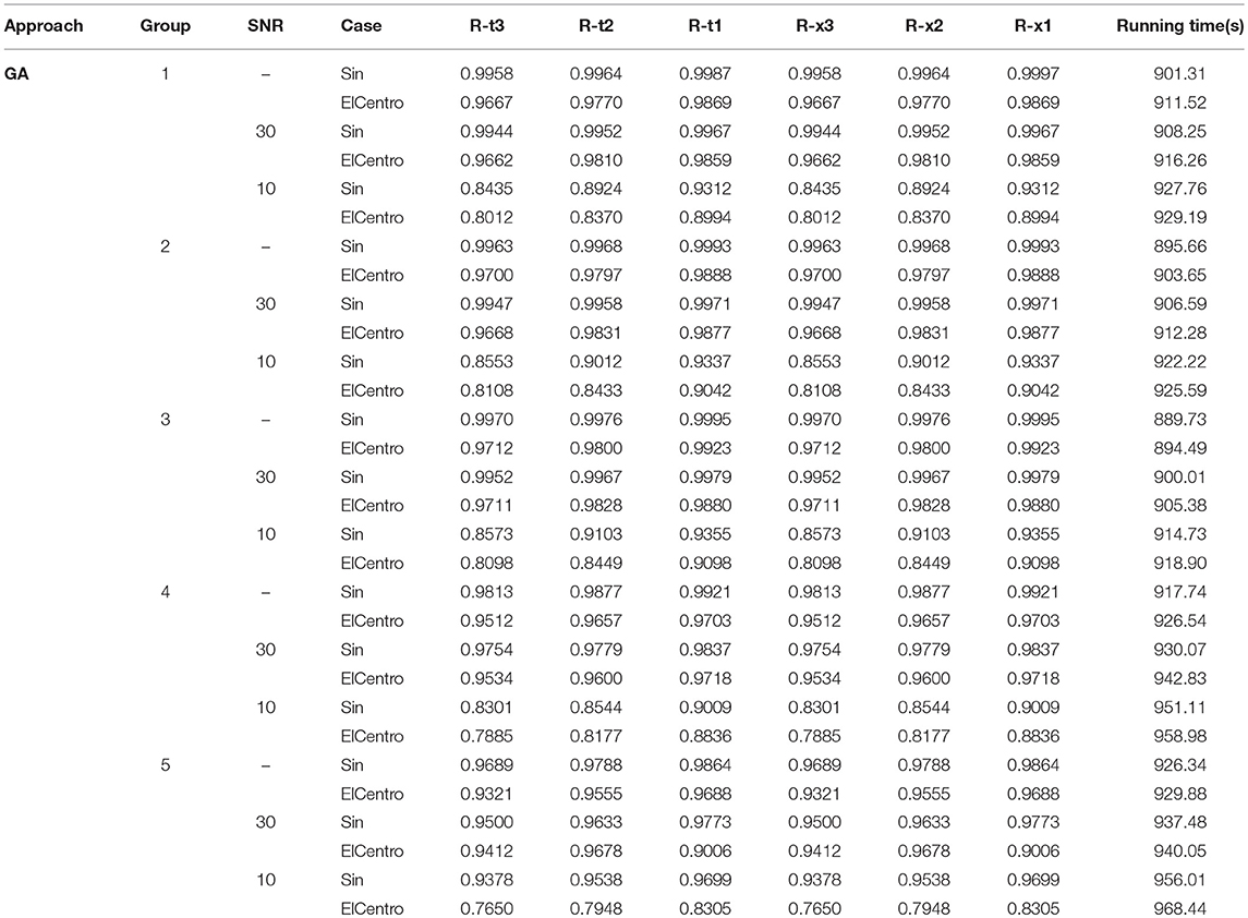
Table 6. Correlation coefficient analysis (GA).

Table 7 shows the influence of change of strength and stiffness degradation parameter on system identification accuracy indicated by correlation coefficients using TMCMC method. For sin excitation, when the strength and stiffness degradation parameter value is fixed at 1.5, as bounds (interval) change from 0–3 to 1–2, the correlation coefficients approach 1, indicating the system identification accuracy improves with the bound interval decreasing.

TABLE 7

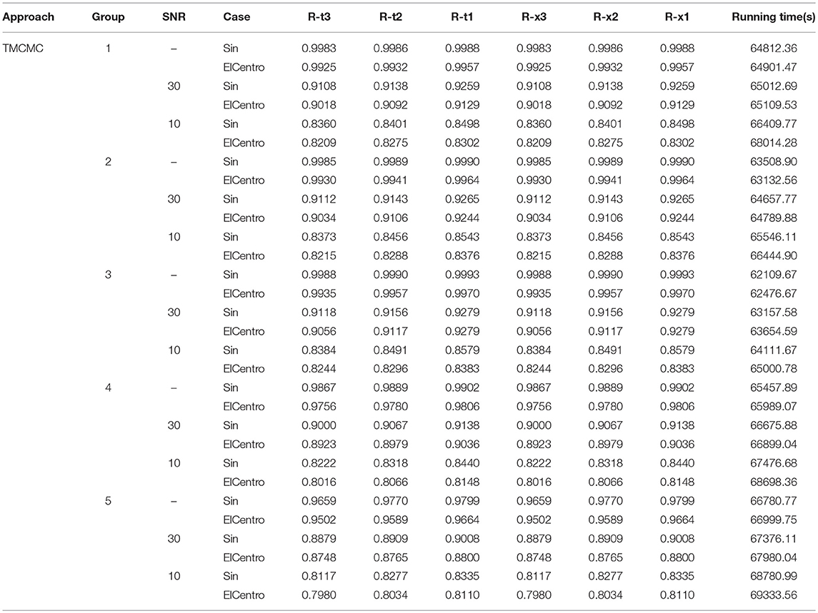
Table 7. Correlation coefficient analysis (TMCMC).

The closer the bounds approach to the true value, the more accurate and deterministic the system identifiion results are. Accordingly, the computational time decreases with the bound interval value decreasing, as shown in detailed cases: Group 1: 64812.36–66409.77 s, Group 2: 63508.90–65546.11 s, Group 3: 62109.67–64111.67 s. When the true value of strength and stiffness degradation increases from 1.5 to 2.1 with given bounds, the identification accuracy decreases, and the computational time increases accordingly. Similar cases can also be found for ElCentro excitation signal.

Comparison of Three Different Algorithm Principles

Intelligent Parameter Varying approach uses radial basis function to map the complex input signal to high dimensional signal, and it is a data driven mechanism. By using appropriate error back propagation mechanism, this method can design a good neural network architecture to process considerable amount of data or high parameter dimension, especially for system identification application. Genetic algorithm and Transitional Markov Chain Monte Carlo approaches are non-data-driven intelligent optimization algorithms. Genetic algorithm optimizes the parameters by using selection, crossover, and mutation operators through elitist strategy. Transitional Markov Chain Monte Carlo method employs model updating to optimize parameters through applying Bayesian inference with TMCMC probabilistic simulations, and the samples eventually populate well in the high probability region of the posterior PDFs close to the true model parameters through a series of intermediate updating processes. The latter two methods are related to optimization theory, and may not perform well (tapped in local optimum) especially when the parameter dimension is relatively large. Therefore, it is very significant to conduct a comparative study on system identification of hysteretic structures using Intelligent Parameter Varying, Genetic Algorithm and Transitional Markov Chain Monte Carlo methods.

The above discussions regarding the choice of signal excitation type, parameter choice for system identification and comparison between three different principles for system identification has demonstrated the necessity, feasibility and importance of this research. It also illustrates the generalization of this research and proves the superiority using IPV over GA and TMCMC for system identification of hysteretic structures.

Conclusions

To better understand the hysterically degrading, structural systems using an earlier version of smoothly varying Bouc-Wen-Baber-Noori hysteresis model in this research, a detailed description of BWBN hysteresis model is presented, and the restoring force and the associated system variables are analyzed using non-linear differential equations containing different parameters. By choosing the parameters in a suitable way, it is possible to generate a large variety of different shapes of the hysteresis loops. A three floor shear structure is modeled which composes of three adjacent subsystems by associating system kinetic equations, restoring force expression and BWBN hysteresis model. By using BWB-Noori model, a new scheme is proposed to effectively and efficiently track and estimate the hysteretic restoring forces using intelligent parameter varying approach, genetic optimization algorithm and the transitional Markov Chain Monte Carlo simulation. Most importantly, comparative study by using these approaches for different cases is demonstrated through parameter error analysis and correlation coefficient analysis of system identification of time varying degrading structures. Major findings are summarized in the following statements.

(1) BWBN hysteresis model is a smoothly varying differential mathematical model, and it can reflect highly non-linear and gradual hysteretic degradation with slip lock behavior observed in numerous structural and mechanical systems, and this model can be widely used to predict the response of degradation phenomena of general structures.

(2) When employing system identification and parameter/model updating approach, the initial parameter spaces of the hysteretic system should be well assigned to satisfy the requirement of reliable system identification process. Tracking of the restoring forces for the hysteretic system using system identification approaches can accurately estimate the changing of restoring force status in time, i.e., the rotation of hysteresis loops indicates structural degradation due to abrupt damages. This proves that system identification techniques can be used as powerful tools for detecting the damage/degradation for structural health monitoring applications. Stiffness and damping terms are lumped into restoring forces represented by structural non-linearity, and this constructs effective IPV modeling.

(3) IPV, GA, and TMCMC methods are employed for the system identification of BWBN model, and a comparative study is conducted for the verification of the effectiveness of these approaches. The results show higher SNR cases have better correlation and smaller parameter errors. From the correlation analysis, we also know that IPV has better anti-noise capability than GA and TMCMC.

(4) Qualitative comparison regarding the computational time of these three different algorithms are ranked for different cases, i.e., IPV Based system identification approach < GA based system identification method < < TMCMC based system identification approach. This demonstrates that compared with traditional parameter optimization and statistical methods, IPV approach is a promising, efficient and effective way for system identification and Structural Health Monitoring applications.

(5) IPV technique using the RBF based ANNs has its superior advantages over the GA based identification and the TMCMC based identification techniques for its fully data-driven adaptive learning ability for high dimensional data. Proper design of parameter initial bounds can improve the computational efficiency for GA and TMCMC approaches. The GA based identification may have relatively uncertain values for the randomness of genetic operations (selection, crossover, and mutation), while the TMCMC algorithm is based on the sampling technique that is not as effective and is uncertain, especially for the case that the system has a relatively large number of parameters.

Author Contributions

YZ as Ph.D. student. MN as main supervisor. WA supervisor. TA was invited, due to his expertise in the area of Genetic Algorithms, to join the paper as a co-author. TA carefully reviewed the technical analysis and independently carried out a system ID using Genetic Algorithm. His contributions were valuable in this regard and thus, his name is added in the newly revised version.

Conflict of Interest Statement

The authors declare that the research was conducted in the absence of any commercial or financial relationships that could be construed as a potential conflict of interest.

References

Abouelwafa, M. N., El-Gamal, H. A., Mohamed, Y. S., and Altabey, W. A. (2014). An expert system for life prediction of woven-roving GFRE closed end thick tube subjected to combined bending moments and internal hydrostatic pressure using artificial neural network. Int. J. Adv. Mater. Res. 845, 12–17. doi: 10.4028/www.scientific.net/AMR.845.12

ORIGINAL RESEARCH article

A Comparison of Three Different Methods for the Identification of Hysterically Degrading Structures Using BWBN Model

Introduction

Structural System Modeling and System Identification

BWBN Hysteresis Model

Structural System Modeling

System Identification Theory

Intelligent Parameter Varying Based System Identification

Genetic Algorithm Based System Identification

Transitional Markov Chain Monte Carlo Based System Identification

Numerical Analysis of System Identification

Parameter Settings

Numerical Analysis Results

Discussions

Choice of Signal Excitation Type and Objective Function

Parameter Choice for System Identification

Comparison of Three Different Algorithm Principles

Conclusions

Author Contributions

Conflict of Interest Statement

References

This article is part of the Research Topic

People also looked at