A weighted network clustering approach in the NBA
Abstract
Evaluating players’ performance for decision-makers in the sports industry is crucial in order to make the right decisions to form and invest in a successful team. One way of assessing players’ performance is to group players into specific “types”, where each type represents a level of performance of its players within. In this paper, we develop a novel clustering approach in order to cluster types of players in the NBA. The proposed methodology is initialized by a k-Means clustering, then the prescribed clusters inform weights of a weighted network, in which players are the nodes and the arcs between them carry those weights that represent a numerical similarity between them. We then call upon a weighted network clustering approach, namely, the Louvain method for community detection. We demonstrate our methodology on six years of historical data, from seasons ranging from 2014–2015 to 2019–2020. Considering these seasons allows us to use a new type of data, called Tracking Data, instated into the league in 2014 which further differentiates our research from other player clustering approaches. We show that our approach can detect outliers and consistently clusters players into groups with identifying features, which give insights into league trends. We conclude that players can be categorized into eight general archetypes and show that these archetypes improve upon the traditional five positions and previous research in terms of explaining variation in Win Shares.
1Introduction
Since the highest-level executives (i.e., decision-makers) in the sports industry have started utilizing modern analytics in helping inform their decisions, sports analytics has gained an increasing popularity for the applications of data science and statistical analysis. The National Basketball Association (NBA) is one of the leagues that is highly utilizing it for making better decisions. While there are many different avenues in which analytics can be applied, one of the crucial concerns of the sports industry is how to evaluate players’ performance. More specifically, in team sports, it is also important to analyze how players’ performances work together, since it is vital to building a successful team. One approach that acts as a starting point for player valuation is determining which “types” of players exist within the league. Generalizing player types can help executives evaluate their value within the context of a team setting.
Basketball traditionally labels players into five positions; Point Guard, Shooting Guard, Small Forward, Power Forward, and Center. This classification, however, is an oversimplified version of the types of players that have emerged over the evolution and growth of the game. It is widely accepted that players of the same position may not necessarily be of the same type. For example, LeBron James and Stephen Curry, are both listed as point guards for the 2019–2021 seasons (basketball reference.com/ 2021). James, at 6’9” and 250 pounds, and Curry, at 6’3” and 185 pounds, have just about as much in common in their style of play as they do in their physiques. James uses his size to post up smaller guards and drive to the basket, while Curry makes 30’ shots from behind the arc (3-PT line) look as though they are as easy as free throws.
Although oversimplication of positions is certainly one motivation to perform cluster analysis of players, the driving force that motivates a better classification of players goes beyond the cluster itself. Decision-makers are often interested in building a team consisting of different types of players that would perform the best on the court. A more granular characterization of players can set the stage for lineup optimization, and therefore can be of very high value to decision-makers. For example, similar to this idea, Chan et al. (2012) perform k-Means clustering for professional hockey and determine the relationship between team performance and player types by using a regression model. Muniz & Flamand quantify the interaction between player clusters by developing a new metric that encompasses the synergy potential between “groups” that each player belongs to. Note that these “groups” are provided by the analysis of this paper. The authors incorporate these findings into an optimization model that prescribes the optimal team building decisions, including which new players to draft, which current players to trade with those of other teams, and/or which free agents to acquire in a way that maximizes team’s total value, including players’ individual values as well as the synergy potential among players on the team.
A more holistic evaluation can also better inform decision-makers’ draft, trade, and free agent acquisition decisions. When faced with comparing and contrasting players such as James and Curry, executives need to know more than their position. Specifically, an efficient cluster analysis would help them in learning about how a player performs, what makes him effective, what his strengths and weaknesses are.
The remainder of this paper is organized as follows. In the next section, we present a literature review to summarize previous research. In Section 3, we describe the data used in our approach. In Section 4, we propose and discuss our methodology in detail. Section 5 presents a case study for a single season (2018–2019) to fully demonstrate the utility of our approach, including a detailed analysis of the resulting clusters, while in Section 6 we explore the previous six seasons to validate our approach and develop insights in trends among the years. Section 7 presents our sensitivity analysis. Finally, we conclude and provide suggestions into future work, specifically in the context of the NBA, in Section 8.
2Literature review
To address the large discrepancy between the traditional positions and the types of players that are labeled by them, one approach that has been explored in the literature is clustering players according to their statistics. In a seminal study that won top prize in the “Evolution of Sports” category at the 2012 MIT Sloan Sports Analytics Conference, the author clusters players using a technique known as topological data analysis and identifies thirteen “new positions”, which he eventually whittles down to ten (Alagappan 2012). Since then, many different clustering approaches have been explored. Zhang et al. (2016) also use the traditional k-Means clustering approach to classify guards (point guards and shooting guards) in the NBA, and identify six different types of guards. Patel (2019) also uses k-Means to cluster players, but first employs dimensionality reductions techniques to the data and identifies four groups of players. Bianchi et al. (2017) use self-organizing maps and fuzzy clustering procedures to develop a new set of five clusters that are different than the traditional five. Dehesa et al. (2019) use player and team statistics and a two-step clustering with log-likelihood distance and Schwartz’s Bayesian criteria to classify players in both the regular season and playoffs; they identify five player types for the regular season and four in the playoffs.
In the literature, there are also studies that focus on clustering players that would help in building successful teams and lineups. Lutz (2012) presents the first work that incorporates this idea and uses multivariate cluster analysis to identify ten clusters of players; the author then analyzes 2- and 3-way interactions of clusters to determine which combinations of players affect winning. Kalman & Bosch (2020) first use model-based clustering to give soft-assignments to players and clusters by assigning a probability that each player belongs in a cluster. The authors develop nine positions, similar to that of Alagappan’s size of ten. Then, they investigate different combinations of these cluster-lineups to determine the most successful ones using random forest models.
Thus far, all existing clustering approaches use a single data set, and primarily, a small set with limited amount of traditional or advanced statistics (e.g., Alagappan (2012) uses only seven statistics to inform his analysis). Alagappan (2012) builds a semblance of a network structure to form player clusters, though topological data analysis is more precisely a geometric approach (Carlsson 2009). Other network clustering approaches in basketball, such as Fewell et al. (2012) and Xin et al. (2017), take an approach such that the nodes consist of players and play-type outcomes and ball movement as arcs. Skinner & Guy (2015) present one of the first network-style approaches to incorporate Tracking data, with the aim of learning players’ skills and predicting the performance of untested 5-man lineups in a way that accounts for the interaction between players’ respective skill sets. Our work differs from theirs in terms of the network structure of the model and the way in which tracking data is incorporated. Specifically, the network in their research models offensive structures and they use tracking data to describe the flow of possessions through the network. This paper takes a different approach, as summarized below.
The contribution of this paper is as follows: to the best of our knowledge, this is the first study that incorporates multiple data sets separately, which allows for more information to inform our clusters and develops a network-based methodology for clustering player types. While the introduction of tracking data allows for more information to be included in the analysis of players, it is also difficult to preserve all of the information encoded within it due to the vast amount of new statistics. Bruce (2016) suggests that the “high dimensionality” of this new tracking data source can be troublesome, as it demands more computational resources and reduces the ability to easily interpret findings. He develops a new metric using Principal Component Analysis (PCA) to summarize the information, although the interpretation of this metric is still not immediately apparent. In this study, we employ PCA on our multiple data sets for reducing the dimensionality, while the results are still interpretable, since information from each data set from which we obtain clusters is encoded into a weighted network. Once PCA is performed on each data set, the proposed methodology is then initialized by several k-Means clustering models that are independently applied to each data set. Then, a weighted network is built, where each node represents a player and each arc represents the similarity between two players (i.e., nodes). Prescribed clusters that are initially obtained from k-Means clustering models inform the weights of these arcs in the network. Using our weighted network, we then perform the Louvain method for community detection, which is a weighted network clustering approach popular in the fields of biology and social network analysis. The network structure allows for a more thorough posterior investigation of the relationships in the clusters. One can call upon network metrics as well as examine the network itself to develop insights that are not previously provided in other clustering approaches. Newman & Girvan (2004) show community detection examples on networks of scientific authors with links between co-authors, on networks of actors in films with links between actors appearing in scenes together, and on networks of interactions between karate club members at an American university. We apply this idea to sports by using k-Means clustering to build ‘similarity’ among players. Our algorithm proposes a new way to think about similarity among players and results in the formation of new archetypes of players in the NBA.
3Data
In this study, we utilize several data sets from NBA.com/stats (2020) for seasons ranging from 2014–2015 through 2019–2020 that span a variety of categories. We extract the data using Python’s nba_api (Patel 2020) package. To keep all data consistent, the per-game averaged, pace-adjusted statistics are obtained directly from NBA.com. These statistics accounts for differences in team pace and possessions. Categories and descriptions of all raw data sets obtained are presented in Table 12 in Appendix A. It shows the breadth of data collected for each player. Although the General and Clutch data sets have overlapping statistics, we consider those separately, since clutch scenarios are specific instances in which the game is within five points in the last five minutes. Players in these situations are on the floor presumably because their coaches believe they have the best chance of winning with them in the game.
Prior to the 2014 season, Player Tracking data that is considered in this paper was not available throughout the league. For this reason, most of the existing clustering approaches use simple statistics, typically coming from either the Traditional or occasionally, the Advanced, data sets described in Table 12 under the General category. In 2014, a real-time tracking technology, SportVU, was introduced into every NBA arena and the data offered by such technology has been made available on NBA.com. Its inclusion in our analysis allows for a more thorough investigation of player tendencies, since it covers statistics not previously seen before such as speed and information on different types of shots (i.e., catch-and-shoot and pull-up) and touches (i.e., elbow, post, paint) and their efficiencies. While these statistics are organized as in Table 12 according to NBA.com, we reorganize the data sets and categorize statistics into six general areas, namely, Scoring, Passing/Playmaking, Rebounding, Defense, Hustle/Miscellaneous, and Clutch, such that each area forms a “Master data set” that includes statistics related to each category, as shown in Table 1.
Table 1
Master data set description
| Data set | Description | Raw Source(s) |
| 2/3 FG(M/A/%) | Shooting | |
| (Drive/Catch Shoot/Pull Up/Paint/Post/Elbow) Touch PTS and % | Tracking Efficiency | |
| Scoring | PTS per (elbow/post/paint) touch | Tracking Possessions |
| PTS (off TOV/2nd chance/fastbreak/in the paint) | General Misc | |
| USG%, Off. Rating | General Traditional | |
| DD2, TD3 | General Traditional | |
| AST %, AST:TO, AST Ratio | General Advanced | |
| Time of possession, touches (all &front-court), avg. sec &dribble per touch | Tracking Possessions | |
| Passing/Playmaking | Drive passes, AST, TOV | Tracking Drives |
| AST, FT AST, Secondary AST, Potential AST, AST:Pass | Tracking Passing | |
| Pass/AST/TOV per (elbow, post, paint) touch | Tracking Elbow, Post, Paint Touch | |
| Screen AST | Hustle | |
| Rebounding | OREB/DREB (Contest/Uncontest/Chance/Distance/Defer) | Tracking Rebounding |
| Off/Def Box-outs, Box-out REBs | Hustle | |
| Defense | STL, BLK, Def Rim FGM/A | Tracking Defense |
| Def FGM/A, % difference (FG%) | Tracking Defensive Impact | |
| Opp 2nd chance/fastbreak/in-paint points | Tracking Defense | |
| Deflections, Charges Drawn, Contested 2/3 PT shots | Hustle | |
| Loose balls recovered | Hustle | |
| Hustle/Miscellaneous | Personal fouls drawn | General Traditional |
| Drive personal fouls | Tracking Drives | |
| Distance traveled, average speed | Tracking Speed Distance | |
| Clutch | USG%, PIE, Possessions | Clutch Advanced |
The decision to reorganize the data into these six categories is deliberate. Basketball is a multi-faceted sport consisting of both offensive and defensive aspects. For example, we break offense into Scoring and Passing/Playmaking to allow for distinction between types of offensive players. Typically, rebounding is lumped in with defense, but there are offensive components to it as well. Thus, Rebounding becomes its own category. In addition, Defense remains its own category. Normal defensive metrics in traditional box-score statistics only cover steals, blocks and rebounds, but our data set is enhanced by both player tracking and hustle statistics, which allows for a more comprehensive evaluation of players’ defensive styles. We also introduce a new Hustle category by combining hustle statistics that were incorporated into the league in 2018 (Martin 2018) with information about aggressiveness and speed to capture the previously intangible value of player effort. Therefore, the statistics within the Hustle raw source, were not included in their respective master data sets (i.e., Passing/Playmaking, Rebounding, Defense, Hustle/Miscellaneous) prior to 2018. Finally, we separate Clutch scenarios from regular scenarios to capture performance in unique situations. Prominent owners such as Mark Cuban have made decisions such as the Jason Kidd acquisition in 2008 (Paine 2010) based on improved performance in the clutch. Separating data sets into these categories allows us to capture and evaluate player performance from a multi-faceted viewpoint and cluster players accordingly.
4Methodology
In the previous section, we identified six categories of statistics that describe the different ways in which players contribute to the game. In this section, using the master data sets that are created based on these categories, we propose a new clustering approach in order to cluster players, namely, Community Detection with k-Means (CD-kM). The proposed methodology has several advantages that allow for a more holistic player evaluation.
Consider sets, parameters, variables and auxiliary functions listed in Table 2. Note that parameters are inputs that must be determined by the modeler. That is, to implement CD-kM, one must decide upon a set of k values,
Table 2
Sets, parameters, variables, and functions
| Sets | |
|
| set of all master data sets |
|
| set of reduced dimension master data sets after performing PCA |
|
| set of all players |
|
| set of k values for k-Means clustering experiments |
|
| set of clusters prescribed by the k-Means algorithm performed on data set dPCA for the given k value |
| Parameters | |
| v | percent variability to keep when performing PCA |
| qr, qc | lower quantile threshold for minutes and games played in regular (clutch) data sets |
| Variables and Outputs | |
|
| the number of times that pair of players
|
|
| binned (discretized) value of
|
| mk | modularity of the community partition for a given k value |
|
| percent of non-singleton groups (i.e., clusters that include more than one player) |
|
| weighted network built for given k value |
| k* | best compromise k value that maximizes both mk and
|
|
| partitions resulting from community detection performed on
|
|
| partitions resulting from community detection performed on
|
| Auxiliary Functions | |
| PCA(d, v) | perform principal component analysis on data set d, retaining v variability; returns dPCA |
| k - Means (dPCA, k) | k-Means clustering performed on reduced dimension data set dPCA |
| Build
| for a given k value, build network such that each player in
|
| CD(
| community detection using Louvain algorithm on
|
| Plot
| for all
|
| Selectk(frontier) | if exists, choose k* such that are balanced, else, choose mk using elbow method, return
|
The proposed methodology is shown in Algorithm 1. It combines the use of two clustering algorithms repeatedly, namely, k-Means and community detection. Both methodologies are implemented using Python. Specifically, we use the scikit-learn library to perform k-Means clustering (Pedregosa et al. 2011), and the community API package to implement Louvain’s algorithm for community detection (Aynaud 2010). We use Louvain’s algorithm since it is shown to outperform other community detection methods in terms of computation time (Blondel et al. 2008). Furthermore, in a recent article comparing different weighted network clustering approaches, Louvain was reaffirmed as “one of the state-of-the-art [weighted network] clustering algorithms” (Arratia & Renedo Mirambell 2021). We use k-Means for the underlying clustering due to its stability. scikit-learn’s k-Means algorithm has a parameter called “init” that represents the method of initialization of the algorithm which takes the value of “k-means++” by default to initialize cluster centers in “a smart way to speed up convergence” (scikit-learn.org 2007–2021). In addition, its “n_init” parameter takes the value of 10 by default which makes the algorithm run ten times with different initial centroid seeds (scikit-learn.org 2007–2021). Therefore the output returned is the best in terms of inertia without the user having to run the algorithm multiple times manually (scikit-learn.org 2007–2021).
Algorithm 1 consists of four main steps. In Step 0, we perform a Principal Component Analysis (PCA), which is a process by which principal components, low-dimensional linear surfaces that are closest to the current observations, are computed (James et al. 2013). Performing PCA reduces dimensionality and preserves variability in data sets. Dimensionality is an important consideration when performing k-Means clustering, because when dimensionality of the data is high, the nearest neighbors in k-Means may not actually be very close and may therefore lead to a poor or misleading fit.
After PCA is performed, in Step 1, the main part of the algorithm is initialized by k-Means clustering. We refer to the clusters yielded by the k-Means clustering as “micro-clusters”. The value of k represents the number of micro-clusters that needs to be pre-defined. In general, in order to determine the best k value, one uses a scree plot or evaluates the silhouette scores among different k values, where the optimal tuning for k is left up to the subjectivity of the analyst. In this study, we implement the proposed algorithm for a set of different k values and follow a similar but an alternative approach to select the best k value, which will be discussed later. For each k value, a k-Means clustering is implemented on each of six master data sets (with reduced dimensions). Therefore, each of these six master data sets has their own set of micro-clusters (i.e., grouping of players). As shown in Table 2,
Once, for each k value, k-Means clustering is implemented on six master data sets and
Algorithm 1
Community detection with k-Means (CD-kM)
1: Step 0: Perform PCA for Dimension Reduction:
2:
3: for
4: dPCA ← PCA(d) ⊳ PCA returns reduced dimension for data set d
5:
6: end for
7: Step 1: Perform k-Means Clustering:
8: Let
9: for
10: for
11:
12: for
13: for
14: if i ∈ c and j ∈ c then
15:
16: end if
17: end for
18: end for
19: end for
20: end for
21: Step 2: Build Weighted Network,
22: for
23:
24: Step 3: Perform the CD Algorithm on Each
25: (
26: end for
27: Plot(
28: Selectk(frontier) ←
29: Return
For each weighted network that is created for a given k value, the Louvain method for community (i.e., cluster) detection is performed. This algorithm is a heuristic with two phases repeated iteratively in order to maximize “modularity” of communities. Modularity is a measure of the density of links inside communities as compared to links between communities. Therefore, the algorithm aims to cluster the nodes such that each community includes elements as similar as possible to each other. The first phase of the algorithm allows local changes in community assignment. Specifically, if removing node i from its current community and placing it in its neighbor j’s community improves modularity, then it is moved accordingly such that the improvement is achieved. The second phase builds another network whose nodes are the communities found in the previous phase. These two phases are repeated until no increase in modularity can be gained (Blondel et al. 2008). The Louvain method prescribes a set of partitions (i.e., clusters of players) that we refer to as “macro-clusters”.
Note that the proposed methodology, (CD-kM), is implemented several times by running multiple experiments with different k values. Therefore, among those, the k value and its associated implementation that achieves the best performance among others should be chosen. One must consider the bias-variance trade-off when choosing the k value. Given this trade-off, using the results of several experiments with different k values, we construct a scatter plot that we call the “modularity frontier” and show an example in Fig. 1 to visualize the bias versus variance trade-off. This frontier is designed to assist in selecting the best compromise k value from the set of experiments run in CD-kM algorithm.
Fig. 1
Example modularity frontier
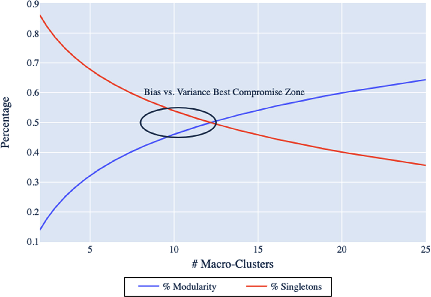
We conceptualize bias as the over-simplification of player types into a small number of groups. In this way, the traditional five positions could be considered as being a biased assessment of actual player types. On the other hand, we conceptualize variance as the over-fitting of player types into a large number of individualized groups, where variance refers to the amount by which the results would change if a different training set (or group of players) was used (James et al. 2013). If each player were to be assigned to their own cluster, then the results would be highly individualized and therefore we would conclude that the variance of the model is high. For example, at an extreme case, if the value of k is equal to the number of players, then each micro-cluster would be of size one which would form a completely disconnected weighted network. Therefore, the community detection algorithm would result in as many macro-clusters as the number of players. These clusters would be completely distinct, but practically useless, as we could not draw any relationships among the group. On the opposite end, if the value of k is too small (e.g., two), then the likelihood that players appear in the same micro-clusters is very high. This would result in a dense weighted network and therefore would be difficult to perform any useful community detection.
5Case study I: 2019–2020 Season
To first demonstrate our methodology in depth, we use as a case study the 2019–2020 season. With any unsupervised clustering algorithm, the user must determine values of certain parameters to use. Thus, we first discuss how parameter values are chosen, then we discuss our results.
5.1Parameters
In order to ensure that we have enough information on each player, we limit observations in all categories (except for the Clutch category) to players above the 25th percentile in minutes and games played. For all data sets except those in the Clutch category, this represents observations with at least 12.6 minutes and 29 games. There are fewer situations in which games are considered in a clutch scenario, and therefore, players are more selectively chosen. Due to this, for those in the Clutch category, we limit observations to players above the 50th percentile, which represents 2.6 minutes and 16 games, respectively. Thus, this results 336 players in the player set,
Table 3
PCA dimensionality reduction results
| Master | Dimensions | ||
| Data set | Before | After | Reduction |
| Clutch | 4 | 3 | 25% |
| Defense | 16 | 10 | 37.5% |
| Rebound | 36 | 15 | 58% |
| Passing | 49 | 26 | 46.9% |
| Scoring | 38 | 24 | 36.8% |
| Hustle | 14 | 7 | 50% |
Note that other binning approaches (e.g., 0, 3, 5) are also explored, as well as using the raw values directly, and our experiments show that dividing the raw values into four bins provides adequate separation among groups. In addition, note that we keep k constant for all data sets within each experiment. This approach also avoids a combinatorial search of using different k-values for each data set. The interested reader is encouraged to experiment with different discretization approaches, k-values, and percent variability schemes that leads to the best results in their use case. The values we ultimately decide upon are a result of the best modularity frontiers. We aim for a modularity of greater than 50% after comparing with recent community detection research. Specifically, Newman & Girvan (2004) find that practical modularity values range between 0.3-0.7 (see references in Singh Ahuja & Singh (2016)). In a subsequent section, we explore different scenarios in which these decisions are altered to develop insights on their sensitivity.
5.2Results
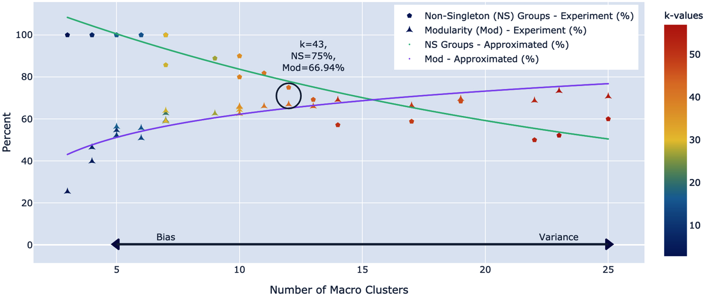
Applying Algorithm \ref alg:cdkm, CD-kM(
Fig. 2
2019–2020 CD-kM Modularity frontier
5.3Macro-cluster (group) analysis
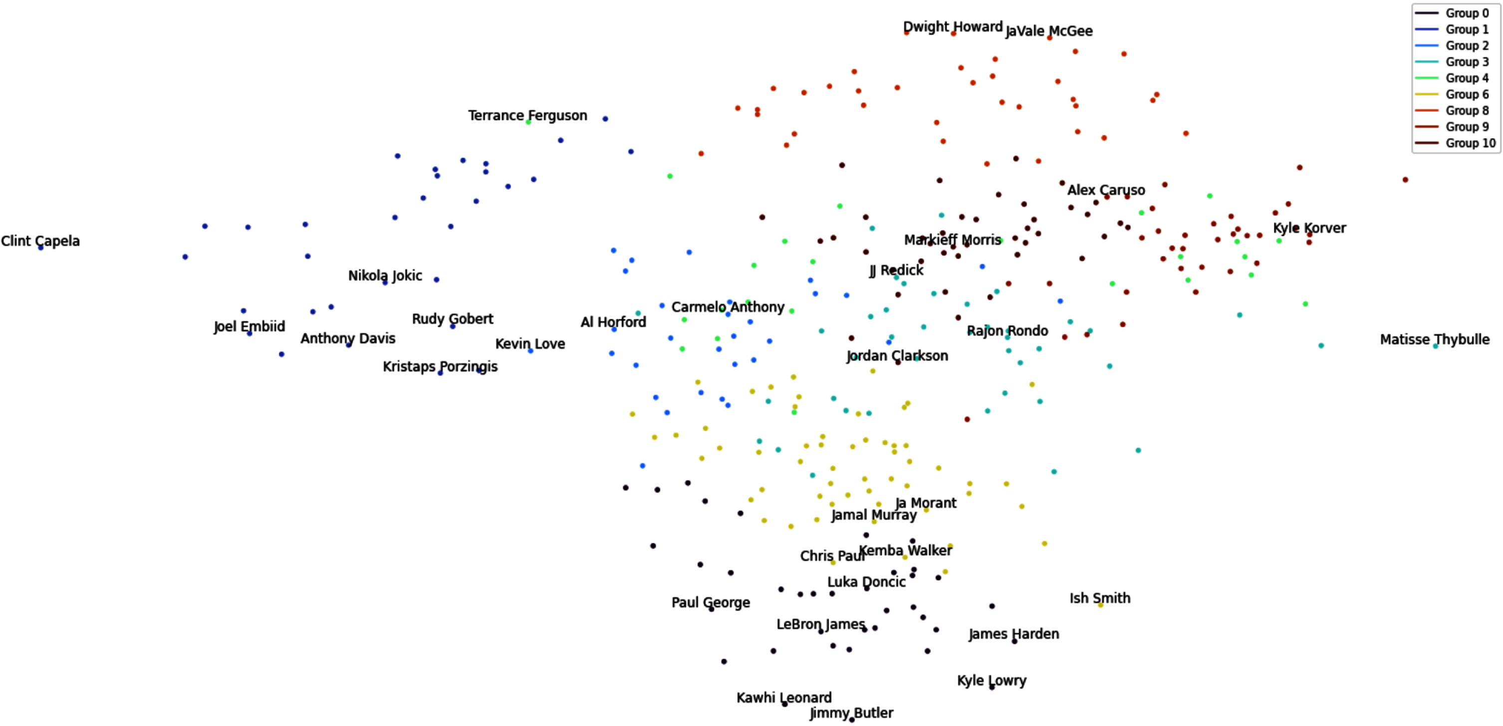
In this section, we examine macro-clusters (i.e., groups) obtained by the proposed methodology for the case study. Fig. 3 visualizes the macro-clusters in a scatter plot form. Specifically the plot shows the weighted network,
Fig. 3
Macro cluster visualization
Note that we examine statistical averages of each macro-cluster, and characterize each of them according to their playing tendencies. Characteristics regarding the performance of players in each macro-cluster are summarized in Table 5 along with notable players in each group. Table 4 displays the size of and average performance metrics for each group and their standard deviations. Sizes of macro-clusters range from 24-57 players, in addition to the three singletons. This would reflect that bias-variance trade-off in choosing k* is managed, with no one single group dominating the others in size. The performance metrics are developed as an attempt to quantify the value of players. PER represents Player Efficiency Rating, which is a measure of per-minute production standardized in a way such that the league average is 15 (Hollinger 2007). Table 4 shows that Groups 0, 1, and 8 on average have a PER higher than the the league’s average. Offensive and Defensive Win Shares (OWS and DWS) are an estimate of the number of wins contributed by a player due to offense and defense, respectively, while Win Shares (WS) is the sum of these two values, and estimate the total number of wins contributed by a player (basketball reference.com/ (2021)). According to Table 4, Groups 0 and 1 dominate in all three of these categories. Comparing OWS and DWS would provide us an idea regarding the main role of each group. For example, all of the Groups 2, 4, 6, 9, and 10 have higher DWS than OWS that suggests that their role is more defensive than offensive. This is understandable, as Groups 0 and 1 seem to dominate the offensive role, while Group 3 are the 3-PT specialists, and Group 8 can score and create for their teammates and also play defense. Finally, USG% is an estimate of the percentage of team plays that a player is involved in while he is in the game (NBA.com/stats/help/glossary/). Groups 0 and 1 also dominate in this category, along with Group 6. These summary statistics match the characterizations in Table 5 and provide a deeper understanding of each group.
Table 4
2019–2020 Group performance metrics: Mean (standard deviation)
| Group | Size | PER | OWS | DWS | WS | USG% |
| 0 | 37 | 19.156 (4.025) | 3.065 (2.506) | 1.812 (1.043) | 4.879 (2.975) | 27.442 (5.238) |
| 1 | 32 | 20.791 (3.147) | 3.194 (1.793) | 2.235 (1.054) | 5.435 (2.534) | 21.615 (5.210) |
| 2 | 30 | 14.574 (3.227) | 1.435 (1.201) | 1.456 (0.933) | 2.897 (1.709) | 18.444 (3.658) |
| 3 | 40 | 12.348 (2.213) | 1.357 (0.982) | 1.200 (0.714) | 2.552 (1.310) | 16.472 (3.358) |
| 4 | 24 | 10.294 (5.059) | 0.494 (0.975) | 0.806 (0.737) | 1.294 (1.515) | 16.075 (3.947) |
| 6 | 57 | 13.906 (3.287) | 1.259 (1.504) | 1.379 (0.731) | 2.627 (1.943) | 21.224 (3.83) |
| 8 | 36 | 15.411 (4.762) | 1.202 (1.118) | 1.068 (0.681) | 2.272 (1.653) | 15.764 (2.897) |
| 9 | 36 | 10.335 (3.225) | 0.441 (0.677) | 0.657 (0.472) | 1.089 (0.971) | 15.874 (3.410) |
| 10 | 41 | 12.160 (3.338) | 0.524 (0.847) | 0.812 (0.525) | 1.334 (1.159) | 17.401 (4.076) |
Table 5
2019–2020 Group summaries
| Group | Characteristics | Notable Players |
| 0 | majority PG/SG; offensive powerhouses (PTS, AST); scoring: drives &pullup shots; record most triple-doubles | LeBron James, James Harden, Luka Doncic, Devin Booker |
| 1 | majority C/PF; record most double-doubles; rebound &hustle specialists; create off screens &passing; efficient scorers inside | Anthony Davis, Rudy Gobert, Joel Embiid, Nikola Jokic |
| 2 | majority PF; inside/outside defenders; ball protectors and efficient scorers inside paint; solid rebounders | Carmelo Anthony, Rudy Gay, Miles Bridges, Kevin Love |
| 3 | majority SG/SF; outside shooters (3-PT, catch &shoot); inside passers (drive &paint AST); high AST/TO ratio | JJ Redick, Grayson Allen, Danny Green, Seth Curry |
| 4 | majority PG/SG; passing specialists (high AST &AST/TOV ratio); quicker players on offense &defense; above average FG3% | Trevor Ariza, K. Caldwell-Pope, JJ Barea, Trey Burke |
| 6 | majority PG/SG; efficient w/ catch &shoot, pullup shots, esp. elbow; offensive playmakers (AST categories); defensive hustlers | Chris Paul, Jamal Murray, Ja Morant, Lonzo Ball |
| 8 | majority C; inside rebounders (both ends) &defenders; AST off screens and from paint; efficient scorers from paint &post | Dwight Howard, JaVale McGee, DeAndre Jordan, Nerlens Noel |
| 9 | majority PG/SG/SF; generally low offensive but high defensive ratings; above average FG3% &AST statistics; quicker players | Kyle Korver, Emmanuel Mudiay, Luguentz Dort, Alex Caruso |
| 10 | majority PF/SG/SF; generally below average offensive statistics, but can shoot FG3; no outstanding characteristics | Doug McDermott, Jordan Clarkson, Markieff Morris |
The proposed methodology offers an improvement from both a topological data analysis approach and other traditional clustering approaches. In our approach, not only can different types of players be identified by utilizing community detection, but also the creation of a network allows one to better understand the groups and the relationships among them. For example, Fig. 3 and descriptions on Table 1 show that Groups 0 and 1 are more clearly delineated, being the high performing triple-double and double-double groups that they are, respectively. Results also reveal that while Group 0 and Group 6 are close, their main difference is that Group 0’s propensity to score and shoot more, while Group 6 are passers first, but still proficient scorers.
Note that in each cluster, there may exist some oddities due to the complexity of player types in the NBA. For example, Kyle Korver’s presence in Group 9 may not be considered as a good fit alongside Alex Caruso. However, Fig. 3 shows that while they are in the same group, their distance is not remarkably close. Specifically, Kyle Korver is located at the edge of his cluster, far from its centroid that represents that he may not fully embody all characteristics of his clusters. The network visualizations for each group in Fig. 6 in Appendix B also show that players cluster towards the center of the network more greatly, which embody the characteristics in Table 5. The further out they appear, the less strongly connected to the group they are.
Note that CD-kM also allows for outlier detection as well as optimal clustering. The outliers (singletons), identified in the 2019–2020 season, are Giannis Antetekounmpo, Ben Simmons and Marc Gasol. Giannis Antetekounmpo was the NBA’s 2019–2020 Defensive Player of the Year and Most Valuable Player, becoming only the third player to win both awards in a single season. Obtained micro-clusters show that Giannis is very dynamic and unique. Similarly, they also reveal uniqueness of Ben Simmons. In the 2019–2020 season, Simmons was First Team All-Defensive and fifth in the league in triple doubles. He is often criticized for his reluctance to shoot from outside, specifically behind the arc, but he is still a prolific scorer, preferring instead to shoot from inside the arc, and doing so with 58.3% accuracy for the 2019–2020 season. For Marc Gasol, a former three-time All Star, the 2019–2020 season was in his thirteenth season in the league. He was an aging player on a team who just won the NBA championship the prior season but lost a majority of their stars to free agency. Our analysis shows that Gasol does not appear in a micro-cluster of his own for any of the six categories, which already sets him apart from Antetekounmpo and Simmons, who distinguished themselves as unique at the micro-cluster level. Instead, Gasol matches with different groups in different categories, which show that his connections split among multiple groups.
5.4Network (micro-cluster) analysis
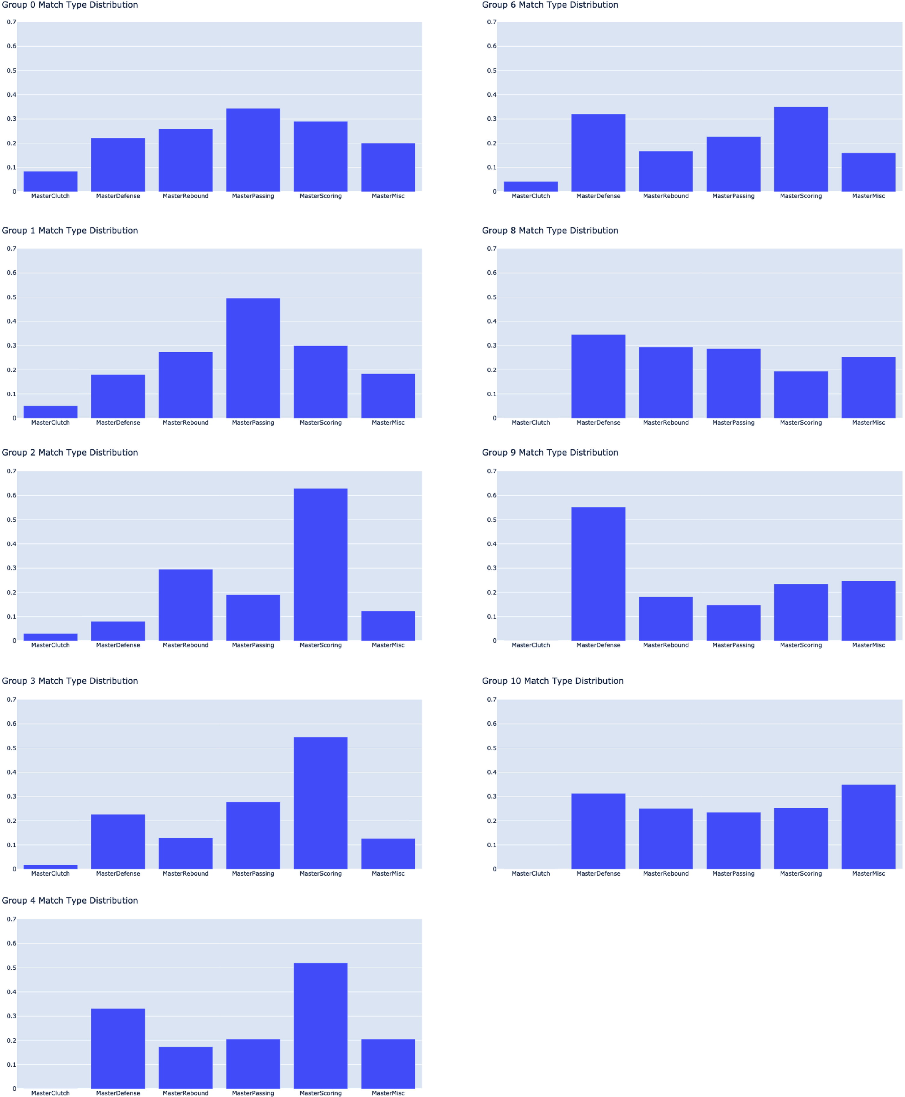
We consider the micro-clusters underlying the creation of the macro-clusters. Recall that an arc between players i and j, shown in Fig. 6 in Appendix B, represents an occurrence of players i and j appearing in the same micro-cluster (k-Means with k* = 43) for at least one of the six master data sets. While these connections are examined between individual players, one can also examine the connections at group levels. To this end, we examine common connections that frequently occur between groups, in terms of categories. We first look at the distribution of categories of matches among each group as shown in Fig. 7 in Appendix C. Recall that the Clutch data set contains only a subset of the players, as these situations are more scarce, so there are fewer opportunities for matches. As shown in Fig. 7, Groups 4, 8, 9, and 10 have zero percent of their matches in the Clutch category. Since these groups are the generally low usage groups, as shown in Table 4, these players may not be involved in many clutch scenarios, in which the outcome of each possession is critical. In addition, our analysis reveals that among the other groups with matches in the Clutch category, Group 0 leads the way with nearly 10% of their matches. This would occur due to the fact that this group contains the high-usage All-Star level players, who may be the ones chosen to have the ball in their hand in a clutch situation.
As shown in Fig. 7 in Appendix C, a majority of the matches in Group 0 are in the Passing (Playmaking) category, followed by Scoring. Their similarity distribution is among the most consistent, with no one category dominating or lagging behind. Group 1 has nearly half of their matches in the Passing category, followed by Scoring and Defense. They contain the second highest percentage of Clutch matches, as this group contains the high-usage effective big men. Group 2’s matches are dominated by Scoring. Recall that these players are effective scoring inside from the point and paint. Group 3’s matches are also dominated by Scoring. Recall that these players are the 3-PT catch and shoot specialists. Group 4 also sees a majority of matches in Scoring, but Defense is a closer second, which would be expected, given that they are highlighted as quick players defensively. Group 6 sees matches in Scoring and Defense in nearly the same percentages, following by Passing. This group is highlighted as being efficient catch/shoot and pullup scorers, playmakers with high assist stats across the board, and the defensive hustlers. Group 8 sees the least matches in scoring (other than clutch in which they do not appear), but more consistent matches in Defense, Rebounding, Passing, and Miscellaneous (Hustle) to a lesser extent. This agrees with their description in Table 5, since this is the group of inside rebounders, who can score from the paint and post, and create assists off the screen and from the paint. Group 9 has a majority of their matches on Defense, and low elsewhere. Finally, a majority of their matches in Group 10 is in Miscellaneous. According to Table 5, it may be concluded that this is a negative match since this group has generally low hustle stats and low distance traveled on both ends of the court. Note that players assigned to clusters may not fully embody all characteristics of the generalizations such as those in Table 5. However, with further investigation into the network structure, the user can gain a better understanding of why clusters were chosen.
In the next section, we apply CD-kM to all seasons with tracking data, beginning with the 2014–2015 season. This allows us to verify our approach for multiple years and also distinguish trends in clusters among the years.
6Historical data
In the previous section, we explore the utilities of our approach on a single season (2019–2020). In this section, we summarize results from the prior five seasons (2014–2015 through 2018–2019) alongside the 2019–2020 results for validation, as far back as NBA tracking data is available for the entire league. Looking at historical data, we identify trends among the types of players in the league. This extends the utility of our approach beyond simply classifying players into groups. The ultimate aim is to be able to use these classifications in a practical sense. For coaches or general managers, the aim may be to build a team of the best combination of players, and these classifications of players provide a starting point. We summarize the results of CD-kM on these six seasons in Table 6.
Table 6
2014–2015 through 2019–2020 CD-kM results
| Season | k* | Modularity | Total # Groups (Non-Single) | Singletons |
| 2014–2015 | 51 | 73.15% | 14 (10) | Zach LaVine |
| Ronnie Price | ||||
| Nikola Pekovic | ||||
| Shane Larkin | ||||
| 2015-2016 | 47 | 65.88% | 13 (9) | Joakim Noah |
| Iman Shumpert | ||||
| DeMarcus Cousins | ||||
| Stephen Curry | ||||
| 2016-2017 | 45 | 69.81% | 12 (9) | Manu Ginobili |
| Luc Mbah a Moute | ||||
| Salah Mejri | ||||
| 2017-2018 | 39 | 66.54% | 10 (9) | Steven Adams |
| 2018-2019 | 49 | 71.96% | 14 (10) | John Wall |
| James Harden | ||||
| Isaiah Canaan | ||||
| (Russell Westbrook, Paul George) | ||||
| 2019-2020 | 43 | 66.94% | 12 (9) | Giannis Antetokounmpo |
| Ben Simmons | ||||
| Marc Gasol |
Table 6 shows that beginning with the 2014–2015 season, CD-kM identifies 14 macro-clusters, four of which are singletons, for a modularity of 73.15%, which is the highest exhibited among all six years examined. For the 2015–2016 season, CD-kM identifies 13 macro-clusters, four of which are singletons, for a modularity of 65.88%. For the 2016–2017 season, CD-kM identifies 12 macro-clusters, three of which are singletons, for a modularity of 69.81%, followed by 10 macro-clusters with one singleton (modularity of 66.54%) in the 2017–2018 season, and 14 macro-clusters with three singletons and one group of two (modularity of 71.96%) in the 2018–2019 season.
With singletons removed, all seasons have a total of nine or ten macro-clusters. By inspecting the group averages for each of the six master data sets for each group and each year, we conclude that groups can be placed into one of eight general archetypes: Supporting Guards, Pass First Guards, Shoot First Guards, Versatile Forwards, Role Playing Bigs, Superstar Guards, and Superstar Bigs. These groups’ advanced statistics are summarized in Table 7.
Table 7
Archetype advanced statistics: Mean (standard deviation)
| PER | TS% | 3PAr | FTr | ORB% | DRB% | TRB% | AST% | STL% | BLK% | TOV% | USG% | WS | Group Name |
| 10.063 | 0.511 | 0.451 | 0.195 | 2.689 | 11.618 | 7.140 | 12.743 | 1.597 | 1.009 | 12.584 | 16.451 | 0.961 | Supporting |
| (2.892) | (0.055) | (0.158) | (0.094) | (1.704) | (3.446) | (2.225) | (8.012) | (0.722) | (0.820) | (4.972) | (3.867) | (0.939) | Guards |
| 11.361 | 0.512 | 0.404 | 0.208 | 2.544 | 10.729 | 6.629 | 16.981 | 1.640 | 0.745 | 13.713 | 17.663 | 1.439 | Pass First |
| (3.559) | (0.061) | (0.156) | (0.101) | (1.547) | (3.141) | (1.991) | (8.809) | (0.563) | (0.688) | (4.435) | (3.906) | (1.287) | Guards |
| 12.211 | 0.545 | 0.468 | 0.201 | 2.175 | 11.281 | 6.723 | 15.356 | 1.657 | 0.924 | 12.388 | 17.700 | 2.355 | Shoot First |
| (2.611) | (0.045) | (0.170) | (0.098) | (1.278) | (3.348) | (2.108) | (8.599) | (0.597) | (0.637) | (3.810) | (3.973) | (1.520) | Guards |
| 13.889 | 0.547 | 0.370 | 0.233 | 5.117 | 16.681 | 10.883 | 10.398 | 1.576 | 1.743 | 11.419 | 18.024 | 3.341 | Versatile |
| (3.453) | (0.044) | (0.188) | (0.099) | (3.024) | (5.849) | (4.098) | (4.577) | (0.596) | (1.245) | (3.283) | (3.585) | (2.054) | Forwards |
| 14.898 | 0.566 | 0.142 | 0.319 | 9.110 | 20.064 | 14.568 | 8.381 | 1.354 | 3.024 | 13.680 | 16.450 | 2.586 | Role Playing |
| (3.800) | (0.060) | (0.199) | (0.158) | (3.379) | (5.401) | (3.813) | (3.769) | (0.602) | (1.860) | (4.251) | (3.410) | (1.612) | Bigs |
| 18.975 | 0.557 | 0.318 | 0.303 | 2.850 | 13.148 | 8.010 | 25.236 | 1.836 | 1.150 | 12.807 | 26.404 | 5.841 | Superstar |
| (4.444) | (0.038) | (0.128) | (0.096) | (1.274) | (4.346) | (2.550) | (10.760) | (0.596) | (0.819) | (3.100) | (4.619) | (3.782) | Guards |
| 14.553 | 0.542 | 0.391 | 0.239 | 2.573 | 12.634 | 7.590 | 17.974 | 1.685 | 1.016 | 12.176 | 21.416 | 3.408 | Scoring |
| (3.592) | (0.049) | (0.143) | (0.093) | (1.451) | (4.667) | (2.758) | (9.924) | (0.670) | (0.989) | (3.581) | (4.347) | (2.590) | Guards |
| 19.422 | 0.576 | 0.117 | 0.345 | 9.457 | 23.477 | 16.461 | 11.915 | 1.355 | 3.295 | 12.660 | 21.829 | 5.639 | Superstar |
| (3.559) | (0.049) | (0.130) | (0.145) | (3.340) | (5.491) | (3.786) | (6.500) | (0.523) | (1.708) | (3.184) | (5.161 | (2.963) | Bigs |
Traditional role-playing guards are split into three archetypes: Supporting Guards, Pass First Guards, and Shoot First Guards. Supporting Guards, similar to Group 9 from 2019–2020, are not outstanding in any of the traditional guard roles, such as scoring and passing, and they are the generally lower usage guards. However, they rebound at a higher rate than their traditional role-playing guard counterparts on both offense and defense.
Pass First Guards, similar to Group 4 from 2019–2020, assist and subsequently turnover the ball at a higher rate than their traditional role-playing guard counterparts. In fact, their assist ratio (not shown in Table 7), or number of assists on average per 100 possessions, is higher than any other group’s.
Shoot First Guards, similar to Group 3 from 2019–2020, are the 3-point specialists of the guards. Not only do they shoot 3-pointers at the highest rate (3PAr), but their True Shooting Percentage (TS%, a shooting percentage that considers three-pointers and free throws values as well as the conventional two-pointers (NBA.com/stats/help/glossary/)) is the highest among the traditional role-playing guards groups. Among the traditional role-playing guard archetypes, they score the most catch-and-shoot, pull-up, and drive points per game. PER and WS both increase among these three traditional guard archetypes in order of Supporting Guards, Pass First Guards, and Shoot First Guards, although they are the lowest in both categories among all archetypes.
The traditional “bigs” (forwards and centers) are split into two archetypes: Versatile Forwards and Role-Playing Bigs. Versatile Forwards, similar to Group 2 from 2019–2020, can shoot from inside and outside the 3-PT arc, they rebound and block at rates higher than the traditional guards but lower than the traditional bigs, yet they assist and steal at rates higher than the traditional bigs but lower than the traditional guards. They excel in the catch-and-shoot scenarios from both 2- and 3-PT range but also get a fair amount of their point on second-chance opportunities and in the paint. Behind the Superstar groups that will be covered shortly, they lead all other groups in double-doubles. Among the traditional roles (both guards and bigs), Versatile Forwards have the highest WS.
Role-Playing Bigs, similar to Group 8 from 2019–2020, are characterized by their inside dominance. Their jobs are mainly to protect the paint, rebound, and create for their teammates in ways that are sometimes underappreciated. They rebound at the highest rates among the traditional roles (both guards and bigs), and aside from the Superstar Bigs, they have the highest block percentage (BLK%). Though their AST% is the smallest among all archetypes, not reflected is their ability to create assists from screens, which is a statistic in which they are second only to the Superstar Bigs. Among the traditional roles (both guards and bigs), Role-Playing Bigs have the highest PER.
For the traditional roles thus far, “bigs” may be viewed somewhat more valuable than guards in terms of PER and WS. This is compensated for in our two archetypes of Outstanding Guards: Superstar Guards and Scoring Guards. Superstar Guards, similar to Group 0 from 2019–2020, set themselves apart from all other guards in all categories. They have the highest usage percentage among all archetypes, which means they are involved in the highest percentage of team plays when they are on the court. In addition, they have the highest PER and WS among all other guard archetypes. They lead all guards in scoring, primarily off of drives and pull-up shots, but also off of second chance and fast break points, assists, and steals. Coupled with their ability to rebound, they tally the most triple-doubles of all archetypes.
Scoring Guards, similar to Group 6 from 2019–2020, separate themselves from traditional guards primarily in their ability to score, which is reflected in a higher USG% and WS in their advanced statistics. They average the second highest points per game behind the Superstar Guards. Their primary form of scoring is off the catch-and-shoot, in which they score the highest points per game among all archetypes. They also excel at scoring off of drives and pull-up shots, on the fastbreak and off of turnovers, second in all these categories only to Superstar Guards. In addition to their offensive ability, they exhibit hustle on defense and have the highest block percentage among guards and second highest steal percentage. Both Superstar and Scoring Guards set themselves apart from the traditional guards through their PER and WS ratings. Specifically, these are guards that are above and beyond the traditional guard roles with their respective characteristics.
Finally, one archetype of “bigs” set themselves apart from the traditional bigs: Superstar Bigs, similar to Group 1 from 2019–2020. These Superstar Bigs have the highest value in terms of both PER and WS. They dominate the paint with both boards and blocks. In addition, they create more for their teammates in terms of assists, as compared to the traditional big archetypes in elbow, post, and paint assists, as well as screen assists, they score efficiently and often from the elbow, post, and paint. They dominate other groups in terms of double-doubles due to their ability to score and rebound consistently.
Identifying these eight archetypes reveals a trend over the course of the past six seasons consistent with the evolution of professional basketball. The game has evolved over the past couple decades, from a post-dominated league with teams revolving around a star center (e.g., the Los Angeles Lakers with Shaquille O’Neal or San Antonio Spurs with Tim Duncan in the early 2000’s), to “Small Ball” (i.e., a style of play that trades size for speed, agility, and 3-PT shooting) teams dominating the league. This transition is apparent in a specific subset of two archetypes identified in Table 8 as two additional sets, since they do not fit into the original eight archetypes. The first archetype is a hybrid between Supporting Guards and Versatile Forwards. The players in this archetype are a near 50/50 split between guards and bigs which would represent a hybrid group. The second archetype is another group of players similar to Role Playing Bigs but that do not quite fit into the regular archetype. These groups appear in the first three seasons (2014–2015 through 2016–2017) where there is a post-dominated league. With two to three other groups of bigs (both Superstar and Role-Playing) in these seasons, these groups distinguish themselves in a sense that they are not good enough to fit the Role Playing Big archetype. In fact, they exhibit statistics below those of Role Playing Bigs in nearly every category, both in Table 8 and in the master data set averages.
Table 8
Misfit archetype averages (standard deviation)
| PER | TS% | 3PAr | FTr | ORB% | DRB% | TRB% | AST% | STL% | BLK% | TOV% | USG% | WS | Group Name |
| 11.735 | 0.546 | 0.478 | 0.217 | 4.123 | 14.901 | 9.529 | 10.288 | 1.364 | 1.636 | 11.451 | 16.796 | 1.477 | Supp. Guards |
| (3.050) | (0.049) | (0.125) | (0.082) | (1.961) | (4.545) | (2.943) | (5.593) | (0.507) | (1.122) | (3.186) | (4.097) | (1.128) | Vers. Forwards (X) |
| 12.145 | 0.531 | 0.295 | 0.263 | 6.278 | 17.487 | 11.871 | 7.643 | 1.277 | 2.038 | 11.816 | 16.415 | 1.658 | Role Playing |
| (3.473) | (0.055) | (0.221) | (0.151) | (3.209) | (4.647) | (3.360) | (3.865) | (0.529) | (1.518) | (3.118) | (3.811) | (1.202) | Bigs (X) |
Note that there may exist overlap among group characteristics and therefore fluidity between players in groups throughout the years. For example, Scoring Guards and Superstar Guards have some overlap in characteristics, and players such as Chris Paul, James Harden, Jimmy Butler, and Kawhi Leonard fluctuate between the two over the six seasons examined. Similarly, Pass First Guards and Supporting Guards overlap, as players such as Vince Carter and Dante Exum fluctuate between the two over the years. Finally, Superstar Bigs share characteristics with both Role Playing Bigs and Versatile Forwards. Players such as Montrezl Harrell, Hassan Whiteside, and JaMychal Green are a few examples of players who fluctuate between Superstar Bigs and either of the similar groups mentioned.
As previously shown in Table 6, CD-kM also identifies singletons for different seasons. Note that Stephen Curry, a singleton in 2015–2016, was also that season’s MVP (i.e., Most Valuable Player) and the first player to win the title with a unanimous vote on a team that broke the single season win record with 73 wins. He also broke Ray Allen’s single season 3-PT shots made record that year. The other singletons in that year consisted of two bigs: Noah, who was seemingly on a decline in his career, as it was his last season with the Chicago Bulls after which time he was traded to the New York Knicks, and ultimately phased into retirement from there, and Cousins, who was seemingly at the peak of his career as he received his first All-Star Game nod and earned 42.9% of the All-NBA Voting Shares (basketball reference.com/ 2021). Shumpert was an average guard on the championship Cavaliers that year, whose stats were likely bolstered from playing alongside LeBron James. Among the other years, the 2018–2019 season has particularly impressive singletons, namely, Wall, Harden, Westbrook/George. Wall, a five time consecutive All-Star at that point, failed to make the All-Star team in this season due to the fact that albeit putting up similar number to his previous seasons, his team saw little success. Harden, coming off of a league MVP and Scoring Title season in 2017–2018, notched another Scoring title, led the league in Usage Percentage (USG%), made the All-Star team for the sixth consecutive season, and finished second in the MVP Award Voting Shares (basketball reference.com/ 2021). Westbrook and George both finished in the top five in Defensive Win Shares, where George led the league in steals per game and Westbrook finished fourth in that category. On the offensive end, George finished third in field goal attempts while Westbrook finished eighth, while similarly they finished third and eighth in field goals missed, as well (basketball reference.com/ 2021). Other seasons have particularly unimpressive singletons, namely Price, Pekovic, Larkin in 2014–2015, and Luc Mbah a Moute, Mejri, Ginobili in 2016–2017 according to their overall lackluster statistics. In addition, note that Zach LaVine is identified as a singleton in his rookie year, which is the only one to do so in our analysis. He has blossomed into an All-Star guard since then, as his scoring and defensive abilities have continued to improve each year.
Finally, we note that the majority of archetypes have an average PER below 15, which is a statistic designed to represent the league average per-minute production. The only groups above this threshold, in fact, are the Superstar Guards and Superstar Bigs. Therefore, our archetypes support the notion that the NBA is a Superstar-driven league (Kaplan et al. 2019). Just below the threshold are the Role Playing Bigs and Scoring Guards. This hints to the importance of having different combinations of (Superstar and/or Scoring) guards and (Superstar and/or Role Playing) bigs on a team.
6.1Performance attribution to player archetypes
In this section, we examine the relationship between the individual metric of WS and the archetypes. This metric has been developed to reasonably approximate a players’ value and is a “top down” metric, or one built upon the production of the whole lineup (Shea & Baker 2013). Table 9 presents the ordinary least squares (OLS) results when regressing the archetypes as categorical variables on WS. That is, we use the archetype and corresponding WS value for each player from the data for seasons 2014–2015 to 2019–2020 as the independent and dependent variables, respectively. We consider the same player in different seasons independently from each other. Furthermore, the comparison group (represented by the intercept) is the Misfit Role Playing Bigs.
Table 9
Archetype ∼ WS OLS Results
| Archetype | Coef | p-value |
| Intercept | 1.5249 | 0.000 |
| Misfit SG/VF | –0.0481 | 0.280 |
| Pass First Guard | –0.0482 | 0.202 |
| Role Playing Big | 0.1785 | 0.000 |
| Scoring Guard | 0.2711 | 0.000 |
| Shoot First Guard | 0.1285 | 0.001 |
| Superstar Big | 0.5929 | 0.000 |
| Superstar Guard | 0.5348 | 0.000 |
| Supporting Guard | –0.1452 | 0.000 |
| Versatile Forward | 0.2843 | 0.000 |
| Variance Explained | ||
| Archetypes | 34.9% | |
| Original Positions | 5.1% | |
All archetypes, less Misfit SG/VF and Pass First Guards, are statistically significant in the OLS regression model. The model has an adjusted-R2 of 34.9%, meaning archetype assignment explains over a third of variation in WS. Comparatively, using original positions as the independent variables in an analogous regression model corresponds to an adjusted-R2 of 5.1%.
Shea (2014) recognizes Alagappan (2012)’s work as the first to suggest the task of redefining player positions, however, he notes that his work is simply not reproducible since the details of his methods or data has not been released (Shea 2014). For this reason, we offer, as a further contribution of this research, access to all data and Python notebooks used to develop this research on Github. Although we cannot compare our work with Alagappan (2012), we compare our Archetypes with that of the fully reproducible work of Cheng (2017). The author uses data from the 2014–2017 seasons from basketball reference.com/ (2021). He uses Per-100 Possessions, Advanced and Shooting Metrics with a total of 56 features. He limits his data to players that played at least 40 games, which resulted in a total of 547 players. Similar to our methodology, he reduces dimensionality of his data using Linear Discriminant Analysis, as opposed to Principal Component Analysis, before performing k-Means clustering. His optimal clustering results in a total of eight groups: Offensive Centers, Combo Guards, Scoring Wings, Defensive Centers, Shooting Wings, Floor General, 3-and-D Wings, and Versatile Forwards. Limiting our data to the same seasons (and therefore to the same players) and regressing on WS, our archetypes have an adjusted-R2 of 36.8% as compared to Cheng (2017)’s of 4.4%. Notice that the R2 values displayed in clusters of Cheng (2017) are actually a reduction from the original positions. We conclude that incorporating Tracking data into clustering techniques using our methodology is an improvement from previous research and traditional clustering techniques alone.
Note that to visualize his groups, Cheng (2017) reduces his data to two principal components using PCA and plots one on each (x, y) axis. While the plots do show separation among the groups, the interpretation is difficult without knowing what the principal components represent. However, in our visualization of the clusters, such as those in Fig. 6 in Appendix B or Fig. 3, the interpretation is straightforward since it is a network of players with associated similarities distinguishing among them.
7Sensitivity analysis
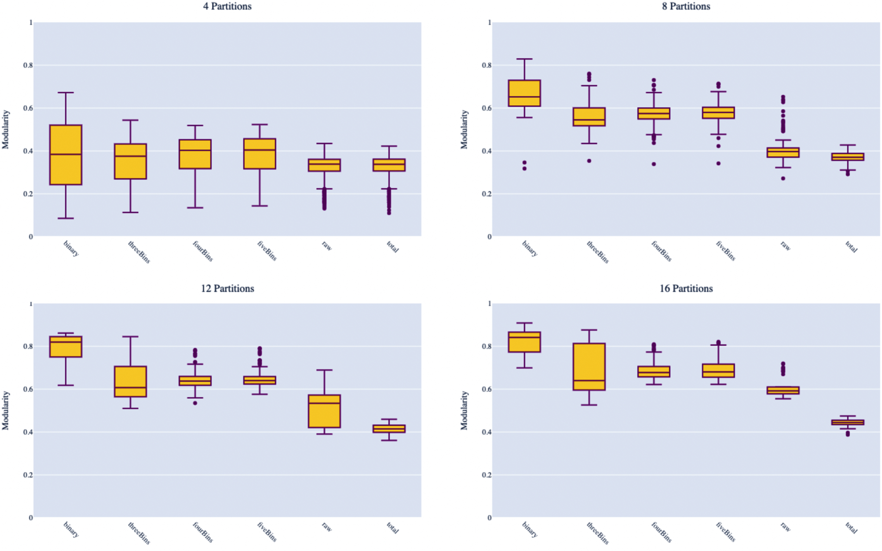
In this section, we perform a sensitivity analysis of the parameters. Specifically, we conduct two experiments using the 2019–2020 data. For the first, we run a full factorial experiment, varying the parameters shown in Table 10, where highlighted values are originally used ones in Case Study I. Figure 4 shows the distribution of modularity for the different binning schemes among all experiments where the resulting Macro-Cluster size,
Table 10
Experimental design #1
| Parameter | Test Values |
| qc | 0.1, 0.25, 0.5 |
| qr | 0.1, 0.25, 0.5 |
| v | 0.7, 0.8, 0.9, 0.99 |
| # Bins | 2 [binary], 3, 4, 5, 0 (weighted [raw] and unweighted [total] δ) |
| Method | k-Means, hierarchical |
Note: We perform an initial sensitivity analysis for the parameters shown in the first column above. The values in bold are those used in the previous sections and serve as a baseline for comparison.
Fig. 4
Experiment #1 results Note: For each box plot, the x-axis represents different binning schemes for the discretization of arc weights: binary, 3, 4, 5, 0 (raw) and 0 (total) as shown in order in Table 10. On the y-axis are the resulting modularity scores from the macro-cluster partitioning. To compare experiments with similar results, we show the resulting partitions (macro-clusters) of size 4, 8, 12, and 16.
Thus, for the second experiment, we use five bins and examine hierarchical versus k-Means clustering separately. We also vary qc, the threshold of players appearing in clutch scenarios to drop, with two different instances: 0.1 and 0.5. Recall that 0.5 was the originally chosen parameter, so we aim to check if including more players into the clutch categories makes a difference. Recall that the value for qr, the threshold of players appearing in the regular data sets to drop, was previously 0.25. In these experiments this value is reduced to 0.10 to include more players. To vary the amount of variation kept in PCA, v = 0.70, 0.80, and 0.90 are used as opposed to the previously used value of 0.99. Note that k is still kept constant in the underlying micro-clusters in order to avoid a combinatorial search to tune k. It also keeps group sizes consistent among the micro-clusters for each data set. In Table 11, we present the results of each experiment and report the number of players in the sample size
Table 11
Experiment #2 design and results
| Parameter Settings | Group Size Information | |||||||||||
| qc | qr | v | Method |
|
| min | max | avg | std | k* | mk* | Time (s) |
| 0.10 | 0.10 | 0.70 | hierarchical | 456 | 8 | 15 | 93 | 57.000 | 27.323 | 41 | 0.585 | 125.04 |
| 0.10 | 0.10 | 0.70 | kmeans | 456 | 9 | 9 | 97 | 50.667 | 32.992 | 47 | 0.617 | 135.74 |
| 0.10 | 0.10 | 0.80 | hierarchical | 456 | 8 | 29 | 92 | 57.000 | 23.670 | 37 | 0.577 | 126.27 |
| 0.10 | 0.10 | 0.80 | kmeans | 456 | 9 | 1 | 93 | 50.667 | 30.590 | 49 | 0.612 | 136.52 |
| 0.10 | 0.10 | 0.90 | hierarchical | 456 | 9 | 17 | 82 | 50.667 | 22.159 | 49 | 0.637 | 127.39 |
| 0.10 | 0.10 | 0.90 | kmeans | 456 | 8 | 28 | 106 | 57.000 | 31.708 | 41 | 0.606 | 136.52 |
| 0.50 | 0.10 | 0.70 | hierarchical | 387 | 10 | 2 | 85 | 38.700 | 24.454 | 13 | 0.747 | 49.88 |
| 0.50 | 0.10 | 0.70 | kmeans | 387 | 7 | 3 | 101 | 55.286 | 29.848 | 9 | 0.713 | 60.11 |
| 0.50 | 0.10 | 0.80 | hierarchical | 387 | 10 | 2 | 83 | 38.700 | 24.051 | 13 | 0.757 | 47.24 |
| 0.50 | 0.10 | 0.80 | kmeans | 387 | 13 | 2 | 69 | 29.769 | 15.369 | 17 | 0.828 | 59.69 |
| 0.50 | 0.10 | 0.90 | hierarchical | 387 | 13 | 2 | 107 | 29.692 | 26.871 | 19 | 0.819 | 48.81 |
| 0.50 | 0.10 | 0.90 | kmeans | 387 | 9 | 3 | 130 | 43.000 | 37.283 | 13 | 0.771 | 60.84 |
Note: The first four columns show the parameter values that varied for each experimental unit.
The last column of Table 11 shows that the run-time of Algorithm 1 grows as the sample size grows, and that hierarchical clustering performs faster. While typically faster run-time is preferred, we defend our use of k-Means due to the stability of its implementation. That is, the randomized seeding technique known as “k-means++” used was shown to obtain an algorithm that is O (log k), competitive with the optimal clustering (Arthur & Vassilvitskii 2007). There is no such guarantee in hierarchical clustering because it is a bottom up approach that requires tuning for the linkage criteria. Note that the run-time is directly related to the cardinality of
Although k is kept constant in these experiments, we do not just optimize k for each data set but instead, use the information from these results to inform the weighted network. Based on our investigation, it is found that if using traditional k-Means clustering on each data set, the optimal k value for each data set according to silhouette score is two. We refer back to Fig. 2 where using small values, less than five, results in poor modularity in the macro-clusters. To this end, rather than optimizing k for the micro-clusters, we tune the value of k by way of the modularity frontier to find comprimising k* that maximizes modularity and balances the bias/variance trade-off.
Table 11 reveals a few observations. First, the amount of variation v kept using PCA does not appear to have a significant affect on the results. Second, there is not a significant different between using k-Means and hierarchical clustering in terms of the results. Third, when there are more players in the data sets (i.e., when qc and qr are low), modularity ranges between 0.566-0.637 and consistently results in eight to nine groups with only one case of a singleton: Oshae Brissett who only averaged seven minutes in 19 games. The value of k* in these scenarios range from 37-49. However, when the sample size is smaller due to fewer clutch instances (i.e., qr is higher), modularity improves to range between 0.713-0.828 with k* ranging between 9-19 and the number of groups ranging from 7-13 with instances of smaller groups.
Recall that the data sets in Section 5 had 336 players. When we increase sample size, in both of these instances, the singletons are distinguished due to their lack of statistical impact. There were five players appearing in groups of three or less: Gary Payton II, Carsen Edwards, Javonte Green, Chris Clemens, and Oshae Brissett. Only Gary Payton II appears in the original case study. He averages nearly 15 minutes per game in 29 games and is classified as a Pass First Guards. The four other players average under 10 minutes per game. These five players, on average, had a VORP of 0.0 with a standard deviation of 0.158. Note, VORP is an estimate of the points per 100 team possessions that a player contributed above a replacement-level player, it acts as an estimate of each player’s overall contribution to the team (basketball reference.com/). Therefore, with more players, it is harder for the algorithm to determine outstanding singletons, such as Giannis Antetokounmpo and Ben Simmons.
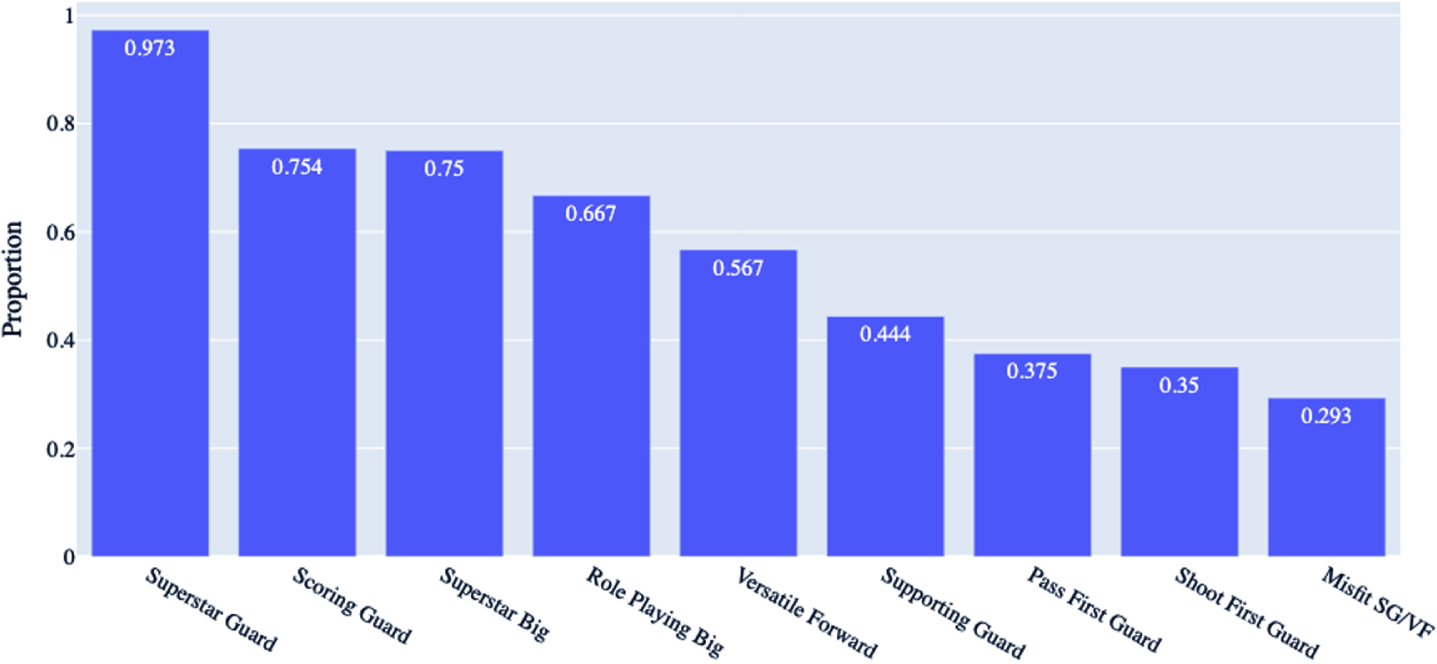
Examining the macro-clusters resulting from each experiment reveals that, most of the time, players are consistently clustered in the same group. Figure 5 shows that 97.3% of players in the Superstar Guards are always grouped together in all our experiments given in Table 11, followed by Scoring Guards, Superstar Bigs, and Role Playing Bigs. This shows that the results for those groups are particularly robust, given their statistics are very distinct. For Versatile Forwards, Shoot First/Pass First/Supporting Guards, and the Misfits, the percentage of matches ranges from 29.3% to 56.7%; nearly a third of the players to just over half always appear in the same group in these experiments regardless of the parameters. This shows that due to the prominence in their statistics or style of play may be harder to distinguish.
Fig. 5
Experimental results - proportion of players always grouped together
Overall, our sensitivity analysis shows that the number of players in the sample, which is affected by qr and qc, has an affect mostly on the outliers (i.e., singletons or group sizes of two to three). In general, the smaller the sample size, the better modularity the algorithm is able to achieve, which is largely influenced by the ability to detect outliers. Overall, with outlier groups removed, the experiments largely result in 8-12 groups, consistent both with previous research and those found in Sections 5 and 6.
7.1Comparison of CD-kM with k-Means
In this section, we provide a brief comparison of the proposed methodology with a traditional clustering algorithm, k-Means. In particular, our aim is to show the benefits of the proposed methodology, and explain why we do not cluster players by simply combining all of the data into a single data set and performing one pass of a clustering algorithm. To address this, we first combine data sets into a single data set for the 2019–2020 season using the same 336 players and perform PCA retaining 99% of variation. We then perform k-Means clustering with several k values. The resulting optimal value of k suggests that it to be between 9 and 11. Given that the number of macro clusters in our methodology is 12, we note that this is similar to what our methodology suggested. Although it is hard to compare cluster strength of these methodologies since clustering is unsupervised, we observe that our methodology provides clusters with more consistent number of members when compared to k-Means clustering. Specifically, k-Means results in group sizes ranging from 12 to 60, with no singletons, while the proposed methodology yields those ranging from 24 to 57. This implies that k-Means is unable to identify players in a way that the proposed methodology does. For example, while we have two clusters; Superstar Guards and Scoring Guards, k-Means suggests a single cluster including players from both of these clusters. We believe that the most significant benefit of the proposed methodology is that it provides more opportunity to obtain deeper insights about players’ characterization. For instance, when k-Means clustering is performed on a single data set, the only information obtained is the centroid of each cluster. However, it does not provide any information about whether a cluster is assigned because they perform similarly in clutch instances, or in passing/playmaking instances, etc. In addition, it does not provide any information on a pairwise level (i.e., player to player), which similarities they carry (e.g., defensive similarities, hustle similarities). Our methodology, on the other hand, by using the master data sets independently, allows one to post-process the macro-clusters and examine their micro-clusters to observe, for example, which players ‘matched’ in clutch instances, or passing/playmaking instances, or defensive or hustle instances. We also note that since the single data set includes much larger dimensional space, it is possible that k-Means clustering leads to poor or misleading results or becomes computationally involved in certain cases.
8Conclusion
In this paper, we develop a novel clustering approach in order to classify players in the NBA into different types by utilizing community detection on similarity graphs. The proposed approach would help decision-makers in making better decisions to invest on the “right” players they need in order to form successful teams.
In contrast to previous research, which uses a small set of simple statistics, we aim to leverage the vast amount of data provided by the NBA. To this end, we first use a set of six master data sets, which characterize six different aspects of how the game is played, namely, scoring, passing/playmaking, rebounding, defense, hustle/miscellaneous, and clutch. The dimension of each of these data sets is reduced by employing a PCA method. Then, on each of these data sets, we perform k-Means clustering to build, so-called “micro-clusters”. Based on the six obtained sets of micro-clusters, the number of times each pair of players appear in the same micro-cluster is counted. That informs weights on arcs of a weighted network which we further built. Since the nodes of the network represent players, the weight on each arc that connects a pair of players show “similarity” between these two players. Once the weighted network is built, we utilize the Louvain algorithm to perform community detection, which prescribes so-called “macro-clusters”, which is the final classification of players. Note that this approach is run multiple times with several k values for the k-Means clustering performed initially. Then based on the macro-clusters obtained from each experiment, we form a modularity frontier, which helps us in selecting the best k value that considers the bias-variance trade-off.
We first demonstrate our approach and its utility on the 2019–2020 season data. We show that not only the proposed approach can identify logical groups, but also it can identify outliers, at both the micro- and macro- group level, in both the positive (e.g., Giannis Antetokounmpo, 2019–2020) and negative direction (e.g., Marc Gasol, 2019–2020).
We also apply our methodology to the data of past six seasons in order to show that our approach captures the league trends. Our results show that in the past six seasons, one can identify a set of groups that are consistent in size. We show that players in each year fit into eight general categories: Supporting Guards, Pass First Guards, Shoot First Guards, Versatile Forwards, Role Playing Bigs, Superstar Guards, and Superstar Bigs. The trends in the changes in archetype makeup of each season reveals the evolution of the NBA from a center-dominated league to a guard-dominated league.
Our approach takes a more holistic approach to classifying players. We also explore many insights provided by the network structure, such as the strength and distribution of matches according to the six different categories of data sets. These insights can be of use to executives who may be considering different trade and free-agent acquisition decisions, in which they must evaluate which types of players they want to acquire. To that end, in a follow-on paper, these archetypes are used in an optimization model in order to decide on which players to acquire in a way that maximizes the total team value, including cumulative individual values and synergy among these archetypes (Muniz & Flamand 2022).
Note that when performing any type of unsupervised clustering, the decisions of the user may affect the results. To this end, we conduct a sensitivity analysis which shows that the results for most archetypes are robust to the parameters proposed in our Algorithm 1. Note that the outliers and less distinguished groups are more sensitive to the parameter settings.
Finally, we note that the proposed methodology, CD-kM, may also be applied to many other areas beyond sports such as customer segmentation in the retail industry. We consider cases in which many different types of retail data sets exist. For example, customer demographics, in-store purchase information, e-mail interactions, and online purchase activities, may be available to the analyst who aims to develop groupings among their customers. In that case, CD-kM can be used to cluster similar types of customers that would inform the marketing strategy of the retailers towards each customer segment. In another setting, financial planners may aim to perform cluster analysis to understand different types of investments, given different types of data regarding the investments, some of which may even be in differing formats. In that case, CD-kM can also be used to cluster similar types of investments to better inform their decisions.
References
1 | Alagappan, M. , 2012, ‘From 5 to 13: Redefining the positions in basketball’, MIT Sloan Sports Analytics Conf. URL: http://www.sloansportsconference.com/content/the-13-nba-positions-usingtopology-to-identify-the-different-types-of-players/ |
2 | Arratia, A. , & Renedo Mirambell, M. , (2021) , ‘Clustering Assessment in Weighted Networks’, PeerJ Computer Science, 7: . |
3 | Arthur, D. , & Vassilvitskii, S. , 2007, in ‘Proceedings of the Eighteenth Annual ACM-SIAM Symposium on Discrete Algorithms’, Society for Industrial and Applied Mathematics. URL: http://ilpubs.stanford.edu:8090/778/1/2006-13.pdf |
4 | Aynaud, T. , 2010, ‘python-louvain’, https://github.com/taynaud/python-louvain.basketballreference.com/ |
5 | Bianchi, F. , Facchinetti, T. , & Zuccolotto, P. , (2017) , ‘Role revolution: Towards a new meaning of positions in basketball’, Electronic Journal of Applied Statistical Analysis, 10: (3), 712–734. |
6 | Blondel, V.D. , Guillaume, J.L. , Lambiotte, R. , & Lefebvre, E. , (2008) , ‘Fast unfolding of communities in large networks’, Journal of Statistical Mechanics: Theory and Experiment, 2008: (10), 1–12. |
7 | Bruce, S. , (2016) , ‘A scalable framework for NBA player and team comparisons using player tracking data’, Journal of Sports Analytics, 2: (2), 107–119. |
8 | Carlsson, G. , (2009) , ‘Topology and data’, Bulletin of the American Mathematical Society, 255–308. |
9 | Chan, T.C. , Cho, J.A. , & Novati, D.C. , (2012) , ‘Quantifying the contribution of NHL player types to team performance’, Interfaces, 42: (2), 131–145. |
10 | Cheng, A. , 2017, ‘Using Machine Learning to Find the 8 types of Players in the NBA’, https://medium.com/fastbreak-data/classifying-the-modern-nba-player-with-machine-learning-539da03bb824 |
11 | Dehesa, R. , Vaquera, A. , Gonçalves, B. , Mateus, N. , Gomez-Ruano, M. Á. , & Sampaio, J. , (2019) , ‘Key game indicators in NBA players’ performance profiles’, Kinesiology, 51: (1), 92–101. |
12 | Fewell, J.H. , Armbruster, D. , Ingraham, J. , Petersen, A. , & Waters, J.S. , (2012) , ‘Basketball teams as strategic networks.’, PLoS ONE, 7: (11). |
13 | Hollinger, J. , 2007, ‘What is PER?’. URL: https://www.espn.com/nba/columns/story?columnist=hollingerjohnamp;id=2850240 |
14 | James, G. , Witten, D. , Hastie, T. , & Tibshirani, R. , 2013, An Introduction to Statistical Learning: with Applications in R, Springer. URL: https://faculty.marshall.usc.edu/gareth-james/ISL/ |
15 | Kalman, S. , & Bosch, J. , 2020, NBA Lineup Analysis on Clustered Player Tendencies:Anewapproach to the positions of basket-ball & modeling lineup efficiency of soft lineup aggregates, in ‘MIT Sloan Sports Analytics Conference’, pp. 1–19. |
16 | Kaplan, S. , Ramamoorthy, V. , Gupte, C. , Sagar, A. , Premkumar, D. , Wilbur, J. , Zilberman, D. , & Chair, R. , 2019, ‘The Economic Impact of NBA Superstars: Evidence from Missed Games using Ticket Microdata from a Secondary Market-place’, MIT Sloan Sports Analytics Conference Conference pp. 1–29. URL: http://www.sloansportsconference.com/wp-content/uploads/2019/02/Economic-Impact-of-NBA-Superstars.pdf |
17 | Lutz, D. , 2012, ‘A Cluster Analysis of NBA Players’, MIT Sloan Sports Analytics Conf pp. 1–8. URL: http://www.sloansportsconference.com/wp-content/uploads///-Lutz_cluster_analysis_NBA.pdf |
18 | Martin, B. , 2018, ‘Dig deeper into the game with newdefensive and hustle data’, https://www.nba.com/stats/articles/dig-deeper-into-the-game-with-newdefensive-and-hustle-data/ |
19 | Muniz, M. , & Flamand, T. , 2022, ‘Sports analytics for balanced team-building decisions’, Journal of the Operational Research Society. URL: https://doi.org/10.1080/01605682 |
20 | NBA.com/stats 2020, ‘NBA Advanced Stats’, https://www.nba.com/stats/ |
21 | NBA.com/stats/help/glossary/ (n.d.), ‘Stat glossary’, https://www.nba.com/stats/help/glossary/ |
22 | Newman, M.E. , & Girvan, M. , (2004) , ‘Finding and evaluating community structure in networks’, Physical Review E - Statistical, Nonlinear, and Soft Matter Physics, 69: (2 2), 1–15. |
23 | Paine, N. , 2010, ‘Thoughts on the 2010 mit sloan sports analytics conference’, https://www.basketball-reference.com/blog/index7f04.html?p=4741. |
24 | Patel, R. , 2019, Clustering Professional Basketball Players by Performance, Master’s thesis, University of California, Los Angeles. URL: https://escholarshiorg/uc/item/0th2s0ss |
25 | Patel, S. , 2020, ‘nba api’, https://pypi.org/project/nba-api/ |
26 | Pedregosa, F. , Varoquaux, G. , Gramfort, A. , Michel, V. , Thirion, B. , Grisel, O. , Blondel, M. , Prettenhofer, P. , Weiss, R. , Dubourg, V. , Vanderplas, J. , Passos, A. , Cournapeau, D. , Brucher, M. , Perrot, M. , & Duchesnay, E. , 2011, ‘Scikit-learn: Machine learning in Python’, Journal of Machine Learning Research, 12, 2825–2830. scikit-learn.org (2007–2021), ‘sklearn.cluster.KMeans’, https://scikit-learn.org/stable/modules/generated/sklearn.cluster.KMeans.html |
27 | Shea, S.M. , 2014, Basketball analytics: Spatial tracking, Createspace Independent Publishing Platform. |
28 | Shea, S.M. , & Baker, C.E. , 2013, Basketball analytics: Objective and efficient strategies for understanding how teams win, Advanced Metrics. |
29 | Singh Ahuja, M. , & Singh, J. , (2016) , ‘Practical Applications of Community Detection’, International Journal of Advanced Research in Computer Science and Software Engineering, 6: (4), 2277. URL: www.ijarcsse.com |
30 | Skinner, B. , & Guy, S.J. , (2015) , ‘A method for using player tracking data in basketball to learn player skills and predict team performance’, PLoS ONE, 10: (9), 1–15. |
31 | Xin, L. , Zhu, M. , & Chipman, H. , (2017) , ‘A continuous-time stochastic block model for basketball networks’, Annals of Applied Statistics, 11: (2), 553–597. |
32 | Zhang, L. , Lu, F.L. , Liu, A. , Guo, P. , & Liu, C. , (2016) , ‘Application of K-Means Clustering Algorithm for Classification of NBA Guards’, International Journal of Science and Engineering Applications, 5: (1), 1–6. |
Appendices
Appendix A: Original Data Sets
Table 12 summarizes the raw data sets pulled from NBA.com used to create the master data sets.
Table 12
Raw NBA.com data sets
| Category | Data set | Examples/Description |
| Traditional | PTS, AST, TOV, STL, REB | |
| General | Advanced | AST:TOV, USG%, TS% |
| Hustle | PTS off TOV, Fastbreak PTS, 2nd chance PTS | |
| Traditional | Same as general, where clutch is defined as: | |
| Clutch | Advanced | Last 5 minutes of game, within 5 points |
| Hustle | ||
| Hustle | Hustle | Contested shots, Deflections, Charges Drawn |
| Speed Distance | Distance traveled and average speed | |
| Rebounding | Off/Def REB information (frequency, distance, opportunity) | |
| Possessions | Time of possessions, type touches, PTS per type | |
| Catch Shoot | Catch &shoot FGM/FGA/2 &3 PT% | |
| Player | Pull Up Shot | Pull up FGM/FGA/2 &3 PT% |
| Tracking | Defense | Defensive Rim FG% |
| Defensive Impact | % difference (opponent FG%) | |
| Drives | Drive PTS, Pass, AST, TOV | |
| Passing | Passes, AST/FT AST/Secondary AST | |
| Elbow Touch | Elbow touch PTS, Pass, AST, TOV | |
| Post Touch | Post touch PTS, Pass, AST, TOV | |
| Paint Touch | Paint touch PTS, Pass, AST, TOV | |
| Efficiency | Player tracking shooting summary stats | |
| Shooting | Shooting | 2 &3 FGM/FGA and % |
Appendices
Appendix B: 2019–2020 Group Networks
Figure 6 displays the network for each group identified by CD-kM for the 2019–2020 case study.
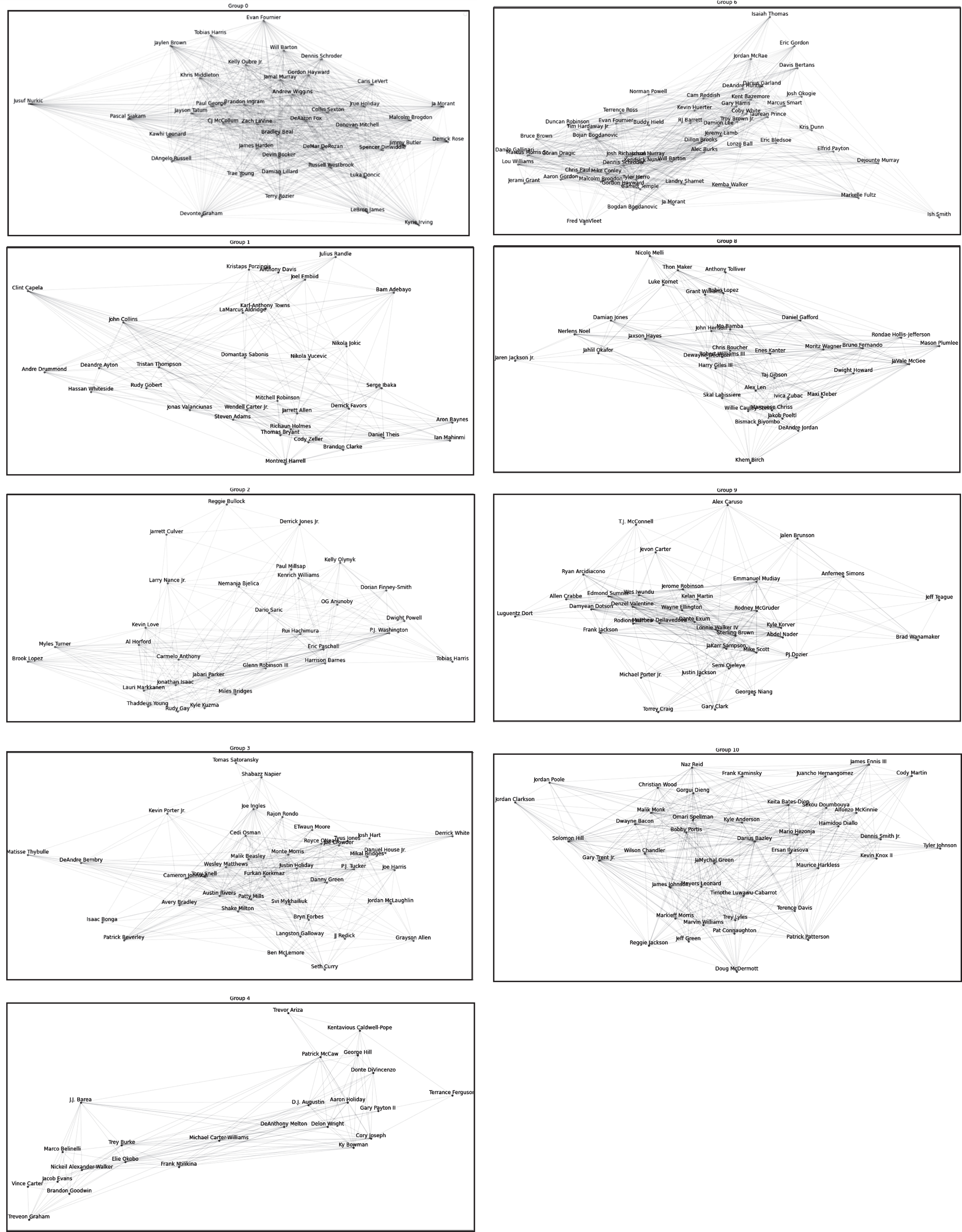
Appendices
Appendix C: 2019–2020 Group Similarity Distributions
Figure 7 shows the count of matches within each master data set for each group identified by CD-kM for the 2019-2020 case study.