


Introduction
High-temporal- and high-spatial-resolution monitoring of the dynamics of Alpine glaciers remains a challenging metrological topic, that can lead to crucial information about ice flow. To fully understand the dynamics of glaciers, surface as well as basal velocities must be determined. For surface velocity estimation, in situ geodetic methods (e.g. global navigation satellite systems (GNSS) and tachymeters) are state of the art in field glaciology for precise velocity determination at daily (Reference Harper, Humphrey, Pfeffer and LazarHarper and others, 2007) to hourly (Reference Sugiyama and GudmundssonSugiyama and Gudmundsson, 2004; Reference Sugiyama, Bauder, Huss, Riesen and FunkSugiyama and others, 2008) timescales, but these methods allow only point measurements, leading to a low spatial resolution. Remote-sensing methods (e.g. optical photogrammetry and synthetic aperture radar (SAR) imagery) have been successfully applied to determine dense surface velocity fields of glaciers (Reference BerthierBerthier and others, 2005; Reference KääbKääb, 2005; Reference FallourdFallourd and others, 2011), but suffer from lower temporal resolution and precision than in situ geodetic methods. The estimation of basal velocity is difficult, because it is rarely possible to reach the base of a glacier. Reference Cuffey and PatersonCuffey and Paterson (2010) reviewed several experiments dedicated to basal velocity measurements. In situ basal velocity measurements have been carried out in a few cases, using instruments set up in tunnels excavated under glaciers (Reference Kamb and LaChapelleKamb and LaChapelle, 1964), in natural cavities (Reference Vivian and BocquetVivian and Bocquet, 1973) or at the bottom of boreholes (Reference Harrison and KambHarrison and Kamb, 1973; Reference Blake, Fischer and ClarkeBlake and others, 1994). An alternative to in situ measurements is to derive the basal velocity from surface velocity measurements by subtracting the internal deformation of the glacier determined by inclinometry (Reference Harbor, Sharp, Copland, Hubbard, Nienow and MairHarbor and others, 1997), but this method requires a large amount of on-site equipment.
In this study, Glacier d’Argentière, French Alps, was selected to test and assess various ice velocity monitoring methods, because it is one of the rare glaciers whose base can be reached. A tunnel constructed under the glacier for hydropower exploitation gives access to a natural cavity, where precise and reliable basal velocity measurements have been carried out since 1986 with a cavitometer instrument (Reference Vivian and BocquetVivian and Bocquet, 1973; Reference MoreauMoreau, 1995). During a 2 month session in autumn 2013, three surface velocity monitoring methods were tested simultaneously with the basal velocity measurements provided by the cavitometer. This paper aims to assess the potential and limits of the collected data to measure as precisely and exhaustively as possible the ice flow of the terminal part of Glacier d’Argentière, which is characterized by a complex mix of non-cracked ice, icefall and crevasses. Using this large number of field observations, the two purposes of this paper are:
To combine three complementary surface velocity monitoring methods to improve the temporal and spatial resolution of the estimated velocity field. To this end, two remote-sensing methods, terrestrial photogrammetry and SAR imagery, were used to map the velocity field of the whole study area and to contextualize the results of GPS in situ measurements, which provide higher accuracy and temporal resolution. The result is a reliable and comprehensive picture of the surface velocity field of the terminal part of Glacier d’Argentière from a first-order stationary flow to very small heterogeneities appearing during speed-up events.
To use jointly two uncommon in situ ice velocity measurement methods, namely a dense array of low-cost single-frequency GPS receivers called Geocubes and a cavitometer, to monitor for the first time the ice flow of Glacier d’Argentière at high temporal resolution, i.e. up to an hourly resolution, simultaneously at the base and the surface of the glacier, during rainfall-induced accelerations of the flow.
The paper is organized as follows: First the study area and the instrumentation are introduced. Next, data acquisition and processing are detailed for each method. Results of the different measurements are compared to evaluate their accuracy, and assess the reliability of each method for ice flow monitoring. Finally, the temporal heterogeneities of the glacier velocity driven by rainfall are investigated using surface and basal in situ measurements distributed around the glacier. These innovative measurements, with their combined high accuracy and high temporal resolution, allow us to highlight various acceleration/deceleration patterns produced by the local response of the ice flow to rainfall and related basal processes.
Study Area and Instrumentation
Glacier d’Argentière is a 9 km long Alpine temperate glacier situated in the Mont Blanc massif, French Alps (Fig. 1). Its flow, regularly studied for decades by glaciologists (Reference Vincent, Soruco, Six and Le MeurVincent and others, 2009), is characterized by a mean surface velocity of ~0.15 m d−1 with interannual, seasonal, monthly and daily variations (Reference Vivian and BocquetVivian and Bocquet, 1973; Reference BerthierBerthier, 2005; Reference BerthierBerthier and others, 2005; Reference PontonPonton and others, 2011). Due to the glacier melting, its terminal tongue is now separated from the rest of the glacier by a 150 m icefall. The upper part of this icefall, Lognan Seracs, is situated 2300 m a.s.l. and can be considered as the end of the main glacier. One kilometre upstream of the Lognan icefall, the glacier exhibits a complex velocity pattern, induced by the coexistence of a central smooth area, crevassed margins and a cracked icefall (Fig. 1). This paper focuses on a 2 month survey of the terminal part of the main glacier, carried out from 13 September to 14 November 2013. Four monitoring methods were combined to measure the ice flow at the surface as well as at the base of the glacier (Fig. 1).

Fig. 1. Glacier d’Argentière study area. Top: panoramic view (17 October 2013). Bottom: general view and equipment.
For the non-crevassed part, 11 ice-fixed and two bedrock-based Geocubes were used. They consist of surveying devices using GPS positioning (Fig. 2a). In order to map the glacier surface as a whole, including inaccessible areas where installation of Geocubes is difficult, two ground-based automatic digital cameras (Fig. 2d) were set up on the orographic right glacier bank. Three TerraSAR-X/TanDEM-X images were used to monitor the surface velocity field of most of the glacier at a larger scale. Bedrock- and ice-based radar corner reflectors were set up to accurately reference these SAR images (Fig. 2c and b, respectively).

Fig. 2. Glacier instrumentation. (a) Geocube, (b, c) radar corner reflectors, (d) digital camera and (e) cavitometer.
In addition to these surface velocity surveys, the basal velocity of the glacier was measured by a cavitometer (Fig. 2e) installed beneath the glacier near the Lognan icefall (Fig. 1).
Glacier Flow Monitoring
Remote-sensing methods provide dense velocity fields of large areas, including inaccessible locations, enabling ice surface velocity field monitoring at the glacier scale. However, most of the remote-sensing methods used to derive surface velocity fields are based on diachronic image matching. First, this limits the use of such methods to textured areas in order to ease multitemporal image correlation. Second, as these methods only apply to the tracking of displacements with an amplitude exceeding one-tenth of the pixel size of the images, they lead to velocity fields with a limited time resolution in the cases of glaciers flowing at tens of centimetres per day.
These characteristics of the velocity fields derived from remote-sensing methods make them valuable mainly in mapping the main trends of the ice surface velocity. In this study, remote-sensing methods were used to contextualize in situ measurements through the mapping of the surface velocity field of the whole of Glacier d’Argentière, and to monitor the downstream acceleration of the flow in inaccessible highly crevassed areas above the Lognan icefall (Fig. 1).
Satellite radar TerraSAR-X data processing
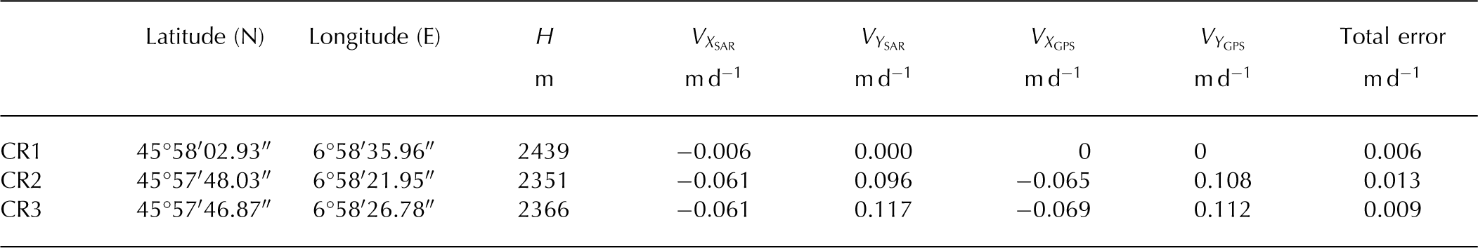
Satellite SAR imagery allows glacier surfaces to be mapped under all weather conditions. Because of the TerraSAR-X/TanDEM-X acquisition plan constraints, only three repeat-pass images were successfully acquired, on 23 October, 3 November and 14 November (after the removal of the other instruments). These images were acquired in ascending passes with a ground resolution of ~2 m in both azimuth and range directions. Due to the glacier surface change, SAR interferometry could not be used to obtain an accurate range displacement measurement. However, with ~1.5 m glacier displacement during the 11 day consecutive acquisitions, amplitude correlation techniques can be applied to measure two-dimensional (2-D) displacement fields in both range and azimuth directions (Reference Luckman, Quincey and BevanLuckman and others, 2007; Reference Ciappa, Pietranera and BattazzaCiappa and others, 2010). During the experiment, three SAR corner reflectors (CR) were installed: a large one (CR1, 2 m side) on the right glacier bank and two small CRs (CR2 and CR3) fixed on the ice close to two Geocubes. Figure 3 presents a colour composition of the three SAR images over the study area after orthorectification. CR1, which was left after the experiment, appears in the three images with a scattering coefficient >30 dB above the surrounding mean value, creating the white point visible in Figure 3. The two other CRs are ~20 dB higher than the surrounding mean value, and appear in orange/yellow, since they were removed before the acquisition of the last image.

Fig. 3. Colour composition of orthorectified TerraSAR-X amplitude images (red: 23 October 2013; green: 3 November 2013; blue: 14 November 2013) over the part of Glacier d’Argentière where the multi-instrument experiment took place, showing the positions of the three corner reflectors (CR).
In a mountainous area, such as the Mont Blanc massif (where altitude ranges from 1000 to 4800 m), measuring the glacier displacement field from SAR data is not straightforward. It was performed using EFIDIR Tools software (Reference PontonPonton and others, 2014) with the following main steps:
-
1. An initial rough coregistration (by translation only) was made by cropping the useful part of the image according to a digital elevation model (DEM) and the orbital information provided by the SAR data.
-
2. A fast-correlation technique (Reference VernierVernier and others, 2011) was applied to the image pairs, with a search window corresponding to a maximum expected displacement and topographic effect (10 pixels in each direction). On the glacier, the measured offset is the sum of the displacement offset and the geometrical offset due to the baseline and the topography.
-
3. The remaining geometrical offset is subtracted using, in the range direction, the predictions from the DEM and the orbits, and in the azimuth direction the results of the sub-pixel correlation around the glacier. The large CR (CR1) is used in this case to estimate and remove the sub-pixel azimuth offset left by the initial co-registration.
-
4. The resulting range and azimuth displacement are converted in m d−1 and orthorectified on the DEM grid (4 m spacing, realized in 2008 by IGN (Institut National de l'Information Géographique et Forestière) and provided by the RGD73-74).
The magnitude of the 2-D velocity field measured with the 23 October 2013–3 November 2013 pair is illustrated in Figure 4. Some abnormal values (0.5 m d−1) are obtained in texture-free areas. These could be discarded by introducing a threshold on the correlation peak. The nonzero values on the motion-free areas reveal that the SAR measurements are still affected by processing uncertainty, which comes either from the amplitude correlation function or from the geometric corrections (orbits and DEM). The DEM error over the glacier, due to surface elevation change, may also affect the results. In the study area, the average ablation rate of the glacier is ~4ma−1 (Reference Berthier and VincentBerthier and Vincent, 2012), ~20 m since 2008. The range offsets due to the baseline and the topography (used in step (3)), show that a 100 m variation between 2400 and 2500 m a.s.l. introduces a 0.06 pixel shift (0.12 m) in range direction. So the error induced by a 20 m elevation change is limited to 2.4 cm for the 11 day displacement; <0.0022 m d−1 error in range direction.

Fig. 4. Magnitude of the 2-D velocity field measured in the range and azimuth direction with TerraSAR-X images (23 October 2013–3 November 2013), normalized on m d−1 and orthorectified.
The final 2-D velocity field measured in SAR images by amplitude correlation corresponds to the projection of the 3-D velocity (east, north, up) in the SAR image plane. The two projection vectors are determined by the incidence angle of the line of sight (LOS) and the azimuth angle of the satellite orbit. For the TerraSAR-X images acquired during this experiment on ascending pass with an incidence angle of 44°, the two unit vectors are
Ground-based digital camera data acquisition and processing
Terrestrial photogrammetry gives access to a dense surface velocity field over a limited area. Here this technique was used to map the velocity field for all points in the area of interest, and particularly in the cracked area near the Lognan icefall.
To this end, two cameras were installed on the right bank of the glacier at 2631 and 2683 m a.s.l., to monitor the glacier flow. These cameras (Leica DMC-LX 4, 10 megapixels; Fig. 2) (Reference FallourdFallourd and others, 2010) were automated and prepared for prevailing glacier climate conditions. They were programmed to acquire five pictures per day between 09:00 and 21:00. This installation provided acquisitions of stereoscopic time-lapse images (stereoscopic time series) of an area 1 km2 and with 158.6 m of baseline between the cameras. The ground pixel resolution is ~50 cm near the glacier. The objective was to compute the displacement of the glacier in two and three dimensions (3-D).
Due to the atmospheric conditions (e.g. wind, humidity, temperature) the positions of the cameras can change. Such motion is highlighted by displacement effects on the motion-free part of the images: the mountains seem to move. Thus, the computation of displacement fields from the images acquired by a camera requires a co-registration step. The objective is to transform all the images of the time series in the geometry of a reference image. Many registration algorithms exist in the literature (Reference Zitová and FlusserZitová and Flusser, 2003). In our approach we used global registration given by
where p is a pixel in the original image and p r the same point in the registered image. It should be noted that p and p r are homogeneous coordinates. To compute the registration matrix, M, a set of points of interest (PoI) was computed and a reference image of the time series was chosen. The choice of the reference image can be arbitrary (e.g. the first image of the time series) or more complex (e.g. an image of the time series that minimizes a distance to the others). The set of PoI can be obtained by SIFT (Reference LoweLowe, 1999), co-registration of image parts (Reference VernierVernier and others, 2011) or other algorithms. The registration matrix, M, was computed for each image, i, using Eqn (2), considering p r as a PoI on the reference image and p the corresponding point on image i. In our case, six areas (three on each bank of the glacier) on motion-free parts close to the glacier were chosen to compute the PoI using the co-registration method (using the normalized cross-correlation function as similarity measure), and the registration matrix, M, was computed as a homograph.
After registration of the left and right time series, the displacement fields were computed by dense correlation (Reference VernierVernier and others, 2011) on the whole image between two dates. Here left images were used to derive the displacement fields because the LOS is near-perpendicular to the glacier flow in this dataset. The result of this step provides the changes over time and the residual error on motion-free parts of the images. Here the mean residual error reaches 0.3 pixel. Figure 5 illustrates the displacements computed from pictures acquired on 20 and 25 September with arrows drawn with a scale factor.

Fig. 5. Displacements (in pixels) computed by photogrammetry between 20 and 25 September 2013. The red arrows highlight the residual errors and the black arrows illustrate the glacier flow. Discrepancies on red arrows correspond to correlation failures.
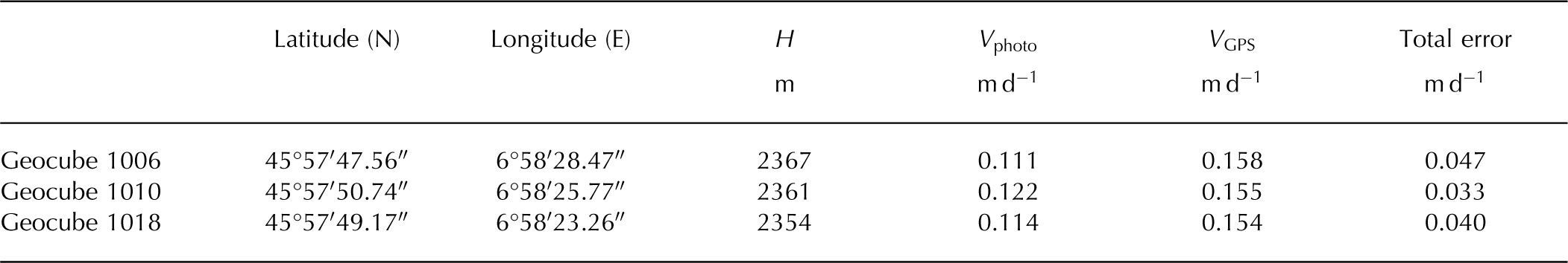
Depth information is required to translate such results in metres and to compute total displacements, taking into account the displacement component parallel to the LOS direction. This information over the whole image was obtained by computing georeferenced DEMs from the stereoscopic installation. MicMac software (Reference Pierrot-Deseilligny, De Luca and RemondinoPierrot-Deseilligny and others, 2011) was used for this step. Previously coregistered pictures were first referenced by bundle adjustment using ground-control points determined by GPS-RTK (real-time kinematic). For technical reasons, only five ground-control points were measured and their repartition in the images is rather poor: they are concentrated in a small area on the right glacier bank. Despite the coarse referencing, a dense correlation algorithm was used to compute a DEM at each date. Next, DEMs and 2-D displacement fields were combined to match 3-D points in DEM computed at different dates (Reference Travelletti, Malet and DelacourtTravelletti and others, 2014). Finally, 3-D displacement and velocity fields were derived from this matching. A mask was used during the processing to reduce the area of interest to the glacier and some stable banks, and thus boost the processing. Figure 6 illustrates the amplitude of the total velocity field computed from pictures acquired on 23 September and 7 October. The result shows good agreement with the crevasse pattern of the glacier. However, some outliers, due to shadow variations, appear on the stable banks. In addition, correlation fails at the right glacier margin due to a high inter-date dissimilarity. The very high velocity and correlation failures at the terminal part of the glacier (right-hand side of the figure) are due to icefalls.

Fig. 6. Velocity field computed by photogrammetry between 23 September and 7 October 2013.
Geocubes data acquisition and processing
Geocubes are multisensor units with networked operation capability developed by IGN for structural and geophysical monitoring (Reference Benoit, Briole, Martin and ThomBenoit and others, 2014). Each receiver includes a single-frequency GPS module for positioning, a radio module for data exchange and a CPU to manage data acquisition. It is designed to be powered by a small solar panel and to support extra sensor modules to supplement the GPS.
During this experiment, Geocubes were used to carry out a GPS survey performed by numerous receivers set up at a large number of accessible points on the central part of the glacier. This leads to an intermediate system between the very punctual conventional geodetic GNSS measurements and the dense remote-sensing results. The low cost of the Geocubes and the ease of setting them up led us to install 11 receivers on the ice and two on the stable bedrock of the glacier banks (Fig. 1). The receivers on the glacier were installed on top of 2 m stems drilled 1.5 m into the ice and powered by a solar panel fixed in the same way (Fig. 2a). Inclinometers included as extra sensors in each Geocube were used to detect stem tilt induced by ice ablation and melting. Thus, it was possible to select only periods with stable GPS receivers for the processing, thereby ensuring that displacements recorded at the GPS antenna phase centre were only due to the flow of the glacier.
GPS data were processed by software developed for Geocubes (Benoit and others, 2014). The processing algorithm is based on L1 carrier-phase double differences, which mitigate dramatically spatially correlated errors if short baselines (<1 km) are used. This makes the L2 frequency data unnecessary. Epoch-by-epoch positions were computed at a 30 s data acquisition sampling rate using an extended Kalman filter. Thus, high-resolution time series of position were computed at each point of the Geocube network (Fig. 7), with a standard deviation of 0.005 and 0.01 m for the horizontal and vertical components, respectively. The main remaining error sources are multipath, i.e. GPS wave reflection and diffusion in the environment surrounding the antenna (Reference Larson, Small, Gutmann, Bilich, Axelrad and BraunLarson and others, 2008). They were mitigated using a time-stacking method (Reference Choi, Bilich, Larson and AxelradChoi and others, 2004) applied when the velocities were derived from the receiver positions. This leads to a velocity time series with a standard deviation of 0.003 and 0.006 m d−1 for the horizontal and vertical components, respectively.
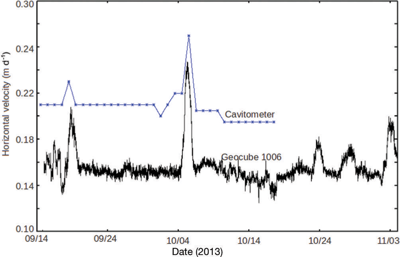
Fig. 7. Horizontal velocity at the base (cavitometer) and at the surface (Geocube 1006) of the glacier. Date format is mm/dd.
Due to receiver tilt, fully reliable data are not available from all points in the experiment. Usable data were collected from the whole network only over the first 5 days, which is sufficient to allow surface velocity heterogeneities to be measured on the central part of the glacier (Fig. 8), where the ice seemed to be a rigid block in the velocity fields derived from remote sensing (Figs 4 and 6), due to the intrinsic precision of these methods. The precision of the results derived from Geocubes allowed us to record, within this area, a higher velocity at the centre of the glacier than near the banks (Fig. 8). A ~7.5% mean ratio between the fastest and the slowest receiver was recorded. The relative displacements of the ice-fixed Geocubes were then used as input data to derive ice surface deformation. Strain tensors were computed using the method described by Reference NyeNye (1959), applied on an arbitrary triangulation between receivers. Computed horizontal strain tensors were then superimposed on orthophotography derived from Pleiades satellite images acquired on 20 September 2013 (Fig. 8). The results show that the deformations of the rigid part of the glacier are very consistent with the direction of the neighbouring lateral crevasses.

Fig. 8. Geocube velocities averaged over five days (14–18 September) and related deformation. The black star denotes the position of Geocube 1006.
Basal velocity measured beneath the glacier
Glacier d’Argentière is a unique site, where basal velocity can be measured continuously throughout the year, thanks to the tunnel dug beneath the glacier. The ability to access the glacier base provides a rare opportunity to directly monitor the basal velocity with high precision and at high temporal resolution.
To this end, a cavitometer is fixed in a natural cavity accessible from this tunnel under ~60 m of ice. It was installed by R. Vivian in 1971 (Reference Vivian and BocquetVivian and Bocquet, 1973), re-established by L. Moreau in 1986 (Reference MoreauMoreau, 1995) and is still used today. It consists of a bicycle wheel rolling on the glacier base (Figs 2 and 9).

Fig. 9. Schematic view of the cavitometer.
After 12 days, only half of the ice-fixed receivers were working properly, and only one receiver (Geocube 1006) acquired reliable data over the whole experiment. However, this single ice-fixed Geocube processed with the fixed one (set up on the right glacier bank) allowed us to characterize the ice flow during the whole period with a high time resolution (Fig. 7).
Slip-free rolling is ensured by the impurities embedded in the basal ice (sand, small rock fragments) and by a counterweight fixed on the arm of the cavitometer which secures the ice/wheel contact. In order to take into account that the rolling surface is not flat, mainly due to rock fragments embedded in the ice or vertical variations of the ice roof, the velocity is computed as (Reference MoreauMoreau, 1995)

The variables used in this equation are shown in Figure 9. The wheel rotation, ω, and the arm tilt, φ, were recorded by analogue potentiometers, and the data were manually digitized for selected periods. During this experiment, data were recorded for the whole session but they were digitized only over the first month (Fig. 7), when they were used for comparison with surface velocity measurements. Figure 7 presents daily basal velocity recorded by the cavitometer from 14 September to 17 October 2013. The resolution of the result, derived from the angular measurement resolution, is theoretically 0.003 m d−1, but its real precision is difficult to establish due to the rolling surface irregularities.
Discussion
Result evaluation by inter-method comparison
Results from the Geocubes present the highest precision (~0.005 m d−1) of the three methods used during this experiment, as shown by the possibility of detecting deformation over the central part of Glacier d’Argentière (Fig. 8). Thus, Geocube data were used as ground truth to evaluate remote-sensing results. To this end, Geocube results were averaged to match the temporal resolution of remote-sensing techniques.
The comparison between SAR and Geocubes was made by projecting the Geocube 3-D velocity, V GPS, in the SAR image plane for three Geocubes set up near the three corner reflectors: two moving with the glacier (CR2 and CR3) and one installed on a stable bank (CR1). Table 1 shows very good agreement between SAR and the Geocubes. This highlights the quality of SAR results for places where the correlation works well (e.g. near corner reflectors, which generate a very strong response into SAR images, or in textured areas (rocks, crevasses, etc.)). In addition, the standard deviation computed on the textured areas of the stable glacier banks reaches 0.026 m d−1. Finally, the precision of the surface velocity field derived from SAR images using an amplitude correlation technique can be estimated at a level of 0.03 m d−1 for most of the study area. However this precision is reached only where well-defined structures exist in both images used for the correlation. For texture-free areas, the correlation technique is no longer valid because of the speckle phenomenon, which is decorrelated after 11 days and produces a high noise level in the amplitude data.
Table 1. Two-dimensional velocity measured at the three corner reflectors by amplitude correlation in the TerraSAR-X images (23 October 2013–3 November 2013 pair) and corresponding GPS measurements
The comparison between photogrammetry and Geocubes was made by comparing the total velocity amplitude at the location of three Geocubes situated on the glacier and operating when pictures were acquired (23 September–7 October). Table 2 shows photogrammetry underestimates the velocity. This is probably due to the coarse image referencing inducing a scale factor, as well as the ground pixel resolution limiting the accuracy of the correlation process. Except for this small bias, the results show good internal consistency and are consistent with the main glacier patterns. Finally, the precision of the velocity field derived from photogrammetry with the ground-based cameras used for this experiment can be estimated at the 0.02–0.05 m d−1 level.
Table 2. Three-dimensional velocity measured at three points by photogrammetry (23 September 2013–7 October 2013 pair) and corresponding GPS measurements
Assessment of basal velocity measurements
Results from the three surface velocity monitoring techniques can then be used simultaneously to check the reliability of the basal velocity measurements carried out by the cavitometer. As shown in Figure 7, the basal velocity at the cavitometer is always ~25% higher than the surface velocity at Geocube 1006. This difference was not, however, due to an instrumental bias, but can be fully explained by the positions of the sensing points along the glacier flow. Indeed, the cavitometer is situated near the Lognan icefall, where the flow velocity increased, even at the surface, as shown by remote-sensing surface velocity measurements (Figs 4 and 6). Except for this velocity ratio, induced by the location of the instruments, the basal and surface velocities present very consistent time variations (Fig. 7).
This simultaneous top and bottom study of the ice velocity allows us to precisely connect the basal velocity measurements carried out by the cavitometer to the ice surface velocity field with an unprecedented time resolution. In addition, this survey leads, for the first time, to monitoring the ice flow velocity of Glacier d’Argentière at its base and surface at hourly resolution (Fig. 10), paving the way for an investigation of its acceleration/deceleration heterogeneities, as shown below.

Fig. 10. Heterogeneities of the acceleration/deceleration pattern at the surface and at the base of Glacier d’Argentière. (a) Long-period surface velocity evolution (14 September–14 October 2013) recorded by Geocube 1006. Rainy periods are highlighted in light blue. (b) Deviation from the mean velocity during two speed-up events (16–21 September and 3–7 October). Time series are shifted (0.03md.. 1) to improve legibility. Green: basal velocity recorded by the cavitometer. Black: surface velocity recorded by Geocubes set up outside the medial moraines. Red: surface velocity recorded by Geocubes set up on the medial moraines. Dashed lines: unavailable data. (c) Precipitation records during speed-up events. (d) Location of Geocube receivers. Date format is mm/dd.
Contribution of precise in situ measurements to rainfall-induced flow heterogeneity monitoring
The Glacier d’Argentière flow velocity was mostly constant during this experiment, but abrupt accelerations followed by a fast return to the mean velocity appear on 19 September and 5 October (Fig. 7). They lead to a velocity peak on 5 October, reaching 160% of the magnitude of the velocity before the event. These accelerations are preceded by heavy rainfall (Fig. 10), which appears to be the major parameter influencing the ice flow velocity variation during the monitored period, probably through increased basal water pressure at the ice/rock interface of the glacier (Reference IkenIken, 1981; Reference Iken and BindschadlerIken and Bindschadler, 1986; Reference Fischer and ClarkeFischer and Clarke, 1997).
However, these acceleration/deceleration events do not have exactly the same pattern throughout the glacier, particularly in a complex and fractured area, as monitored here (Fig. 10). The high precision and the high temporal resolution of the in situ measurements allow analysis of the various glacier responses to rain as a function of the sensingpoint location.
Focusing on surface measurements carried out by the Geocubes, the majority of the receivers present very similar acceleration/deceleration patterns, but two receivers (Geocubes 1010 and 1018) have a different response (Fig. 10b). Their acceleration is delayed compared with the rest of the glacier, and the duration of the speed-up event is longer than for other receivers. A photograph of the area (Fig. 10d) shows that the receivers with the delayed acceleration are both situated on debris-covered medial moraines, while the others are distributed around them but always outside of such moraines. Thus, medial moraines seem to modify slightly and very locally the response of the ice flow to glacier accelerations induced by rainfall. These structures are then presumed to have an effect on basal processes which control the glacier velocity, perhaps due to their excess weight or to a slightly different ice structure beneath them.
The comparison of the Geocube and cavitometer velocities (Fig. 10) highlights that basal and surface accelerations are simultaneous and appear ~1.5–2 hours after the rainfall begins. However, basal velocity seems more sensitive to rainfall intensity, with a pattern directly controlled by rainfall events. The response of the surface is smoother. This higher sensitivity of basal velocity to rainfall events may be due to the local structure of the glacier (thickness of ~60 m of cracked ice above the cavitometer, thickness of ~200 m of compact ice under Geocube 1006) or due to the proximity of subglacial water channels.
Finally, precise in situ measurements carried out at high temporal resolution allowed the monitoring of the heterogeneities of the acceleration/deceleration patterns following rainfall events. Results show that in the study area the glacier does not accelerate totally uniformly. This suggests that the local structure, thickness and topography of the ice locally influence basal processes and then slightly modify the ice flow. The heterogeneous acceleration/deceleration patterns we have documented could be used in further work, together with additional data, such as water run-off downstream or glacier bedrock topography, to model the ice flow of the terminal part of Glacier d’Argentière, which presents a complex ice structure.
Conclusion
This experiment focused on the adaptation of four monitoring methods to measure Glacier d’Argentière ice flow velocity. Each of them leads to partial observations, but their combination helps improve the precision, the reliability and the comprehensiveness of the derived ice velocity measurements. The results highlight strengths and drawbacks of each method during glacier monitoring. They reveal an innovative characterization of the ice flow for the complex terminal part of Glacier d’Argentière near the Lognan icefall, constituting the current end of the main glacier.
The combination of remote-sensing and in situ GPS surveys leads to a continuous ice surface velocity field whose precision depends on the accessibility and nature of the monitored locations. It allows the study of deformations of the ice surface which are clearly the cause of crevasses opening. The acceleration of the ice mass before the Lognan icefall was also precisely documented.
In addition, our survey has produced a simultaneous high-time-resolution record of the ice flow velocity at several locations on the glacier, at its surface as well as at its base. Thereby the flow pattern heterogeneities occurring after heavy rainfall are documented in detail. The structure of the surrounding ice, as well as the position of the sensing points, influence the response of the ice flow to rainfall events. In particular, a slight time shift in acceleration is recorded for medial moraines. The extracted acceleration/deceleration patterns can now be used as the basis for further investigation into the ice flow of the complex terminal part of Glacier d’Argentière (e.g. through numerical modelling).
Acknowledgements
We thank Electricité d’Emosson SA company for the subglacial measurements beneath Glacier d’Argentière, Olivier Couach and Gaiasens SARL for providing meteorological data, the German Space Agency (DLR) for providing the TerraSAR-X data (project MTH0232), the French space agency (CNES) TOSCA/CESTENG project for funding, Jean-Marie Nicolas and André Pahud for help with the cavitometer and recording, and Christian Vincent and Pierre-Marie Lefeuvre for methodological advice. We are also grateful to M. Lüthi and two anonymous reviewers, whose comments and corrections significantly improved the manuscript.


