


1. Introduction
Polar ice cores are essential tools for the reconstruction of past climate. Especially valued are the air bubbles entrapped in the ice, which constitute unique archives of the Earth’s past atmosphere. It is, however, not only the ancient air entrapped in bubbles that has palaeoclimatic significance; the arrangement and geometrical properties of the bubbles provide information about past conditions of snow accumulation, that are used in ice-core dating, proxy modelling and ice-sheet flow simulations.
As a result of continual densification of the deposited snow, the pore space between single snow crystals reduces with time and depth. Through this process of metamorphism, the snow changes to firn and finally to ice. The transition to ice occurs when a critical density is reached, in which the pore channels close off, turning into isolated air bubbles. The depth range at which this transition occurs is called the firn/ice transition (or pore close-off) depth. The distribution of air bubbles in ice is believed to store important information about the past firn structure, which has a direct connection with past climatic conditions. Reference Lipenkov and HondohLipenkov (2000) observed that bubbles formed in cold periods in the Vostok (East Antarctica) ice core are more numerous but smaller than bubbles formed during warm periods. Reference Spencer, Alley and FitzpatrickSpencer and others (2006) developed a method to reconstruct past accumulation rates in ice cores from the air bubble density and the appropriate past temperature.
Once the air bubbles have formed at the firn/ice transition, their number and size distribution, as well as their spatial arrangement, do not change significantly until the depth where the bubble/hydrate transition reaction starts to take place. The bubbles are merely compressed with depth, but that does not affect their size distribution. Therefore, air bubbles are the best proxy for the firn/ice transition in the past. They are the direct microstructural memory of the ice onto the firn/ice transition.
Due to the increasing overburden pressure, the bubbles enclosed in ice shrink with depth until they become thermodynamically unstable and convert into air hydrates. In the EPICA (European Project for Ice Coring in Antarctica) Dronning Maud Land (EDML) ice core we observed air hydrates below ~700 m depth. This depth is the beginning of the bubble/hydrate transition (BHT) zone, where air bubbles and air hydrates coexist. The length of the transition zone in the EDML core is ~500 m.
Air bubbles in glacial Antarctic ice are of particular interest as a microstructural memory of the firn/ice transition. They may help to solve the Δ-age dilemma (Reference LandaisLandais and others, 2006). Neither glacial firn nor a modern analogue of glacial firn exists with which firn models can be calibrated. The long-standing dilemma is that, in contrast to δ15N measurements (a parameter that describes the depth of pore close-off in modern firn reasonably well), firn models predict a significant deepening of the firn/ice transition for glacial climate conditions. This aspect has great relevance for the interpretation of the phasing between temperature and CO2 concentration during climate change; this concerns any temperature/CO2 lead/lag analysis. High-resolution studies of the variability of air bubbles in glacial Antarctic ice are expected to shed first light on the structure of the glacial firn/ice transition, to determine whether a fundamental assumption of all present-day firn models, i.e. homogeneous firn with no layering, is fulfilled.
In this study we present a systematic investigation of the number, size and arrangement of air bubbles in the EDML deep ice core over the whole bubbly-ice zone, including the BHT zone. Altogether, we analysed 101 samples (comprising more than 75 000 micrographs) from the depth range 175–1225 m, starting ~100 m below the firn/ice transition and lasting until the end of the BHT zone of the EDML core. Our study focuses on continual high-resolution investigations of the individual samples (ice-core sections of 10 cm length). These high-resolution studies of bubble distributions give us important information about the relationship between bubble number and size on a small scale, and can be directly linked to stratigraphic features in the ice (e.g. cloudy bands, which appear as dark layers in the ice and are characterized by a high content of impurities).
In earlier studies (Reference NaritaNarita and others, 1999; Reference Lipenkov and HondohLipenkov, 2000; Reference Spencer, Alley and FitzpatrickSpencer and others, 2006) variations in bubble number were mainly related to past temperature and local accumulation rate. In our study we consider a climate proxy, the concentration of impurities, as the main reason for variations in bubble number and size distributions in ice from glacial periods. Impurities have a strong influence on the microstructure of ice (Reference Alley, Perepezko and BentleyAlley and others, 1986; Reference Faria, Freitag and KipfstuhlFaria and others, 2010).
2. Experimental Methods
The EDML deep ice core was drilled at the EPICA Dronning Maud Land site (75° S, 0° E; 2892 m a.s.l.) at Kohnen Station, Antarctica, during the austral summer seasons 2001–06. Samples were taken at intervals of 10 m and prepared as described by Reference KipfstuhlKipfstuhl and others (2006). Their dimensions are ~0.5 cm thickness, 4.5 cm width and 10 cm length along the core axis. Both surfaces were microtomed. To polish the sample surfaces they were allowed to sublimate a short while (15–60 min). Silicon oil was applied on the surfaces before cover glasses were frozen on both sides of the samples, to avoid rime or frost formation between the cover glass and the sample surface.
To document the evolution of the microstructure (i.e. grain size, grain shape, grain-boundary features, slip bands, air bubbles, air hydrates, micro-inclusions and c-axis fabrics) along the entire core, in other words through the entire ice sheet, as comprehensive as possible a microstructure mapping project was initiated. The basic idea was to document as many microstructural features as possible, immediately after drilling at the drill site as digital images and to analyse these images later. The sections were mapped under the microscope to record grain boundaries for grain size and shape analysis (Reference KipfstuhlKipfstuhl and others, 2006). In addition, using the same sections, slip bands, micro-inclusions, air bubbles and air hydrates were mapped at the surface and in two or three focusing planes inside the 5 mm thick section. The images were taken at the drill site within a few days of the cores being retrieved, to avoid relaxation phenomena due to pressure loss. The system used to map the samples consisted of an optical microscope (Leica DMLM), a CCD video camera (Hamamatsu C5405), a frame grabber (SCION LG3) and an xy-stage (Märzhäuser XY100). Images were usually taken in transmission. The process of image acquisition (i.e. the positioning of the sample on the xy-stage and subsequent image capture) was controlled by the public domain NIH Image software (developed at the US National Institutes of Health and available on the internet at http://rsb.info.nih.gov/nih-image/), together with the LG3 frame grabber, both running on an Apple G3 computer. As colour cameras offer no advantage for our purposes, all images were acquired in greyscale. The resolution of the air bubble mapping system is ~5 μm pixel−1. A single image records an area of 1.8 × 3.0 mm2, with an overlapping region of 0.5 mm to facilitate the later reconstruction of the whole mosaic. The mosaic image of the air bubbles of a 10 cm long and 40–50 mm wide sample consists of ~750 images. This is about half the number of images needed to map the same section under the microscope at a resolution of 3.25 μm pixel−1 for grain boundaries and other microstructural features.
The analysis of bubble number density and the geometrical properties of the bubbles relies on the image analysis method of Reference UeltzhöfferUeltzhöffer and others (2010). All images of one sample were automatically merged into a mosaic. The air bubbles were then detected. The position of each bubble, its perimeter and its area were calculated. The bubble number density of a region of the sample was calculated from the measured total bubble number in this region and the region volume. The length and width of the region are given by the dimensions of the respective image, while its thickness coincides with the sample thickness that was measured with a slide gauge. To calculate the equivalent bubble radius, r, and volume, V, from the measured bubble area, A, in the two-dimensional sections we adopted the approximation that the bubbles are spherical:
At shallow depths, just below the firn/ice transition, air bubbles are large and, consequently, there are many clusters of overlapping bubbles in the images. As the image analysis software is not able to break down bubble clusters with more than three bubbles, the misclassification rate is relatively high at shallow depths (Reference UeltzhöfferUeltzhöffer and others, 2010). Therefore we started our systematic investigations at a depth of 175 m. There the misclassification rate is <5%, and quickly becomes negligibly small with depth. Our measurements cover the zone of bubbly ice and the transition zone of the EDML core, which ends at a depth of 1225 m.
3. Bubble Size Distributions, Microbubbles and Ostwald Ripening
The size distribution of air bubbles established by our image analysis is shown for various depths of the EDML deep ice core in Figure 1. The distribution is bimodal, as has already been reported by Reference UeltzhöfferUeltzhöffer and others (2010). The bimodal character becomes less prominent in deeper ice (below ~800 m). A bimodal bubble size distribution in polar ice was first observed by Reference Lipenkov and HondohLipenkov (2000) in the Vostok core. According to the nomenclature introduced by Lipenkov, we call the smaller bubble fraction ‘microbubbles’ and the larger ones ‘normal bubbles’ . The number of microbubbles in the EDML core is small compared with the number of normal bubbles; however, accurate proportions cannot be given, as our image analysis method increasingly misses microbubbles as their radii fall below 10 μm.

Fig. 1. Size distribution of air bubbles for selected depths. Overlapping bins (bin width 5 μm, steps 0.25 μm). Note the bimodal character of the distributions.
The distributions of microbubbles and normal bubbles partially overlap. We refrain from a further quantification of each contribution for two reasons: (1) the image analysis method used is quantitative only for normal bubbles and (2) a systematic reduction of the microbubble fraction in both number and diameter has to be expected, as a consequence of Ostwald ripening of the bubbles. Such ripening processes have been quantitatively established for air hydrates in the Dome Fuji (Antarctica) ice core (Reference Uchida, Miyamoto, Shin’yama and HondohUchida and others, 2011); similar observations have also been made for the Greenland Ice Core Project (GRIP) deep ice core (Reference Pauer, Kipfstuhl, Kuhs and ShojiPauer and others, 1999). The diffusion of air molecules within the ice matrix appears to be a constantly active process (Reference Ikeda-Fukazawa, Hondoh, Fukumura, Fukazawa and MaeIkeda-Fukazawa and others, 2001; Reference Salamatin, Lipenkov and HondohSalamatin and others, 2003; Reference Nedelcu, Faria and KuhsNedelcu and others, 2009), which eventually leads to a preferential growth of larger air hydrate crystals at the expense of smaller ones, as a consequence of Laplace’s law. One has to expect an analogous process also to take place for air bubbles: larger bubbles will grow at the expense of smaller bubbles. Thus, the microbubbles will eventually disappear, leading to an apparently monodispersed distribution at greater depths; the distribution at 903 m(and below) provides some evidence for this ripening process (Fig. 1). Yet, the dominant process influencing the diameter of the normal bubbles is the volume reduction due to the pressure increase, which results in an overall trend to smaller diameters as a function of depth, shown in Figure 2. Thus the Ostwald ripening so clearly seen in the largely incompressible air hydrates, will be much harder to quantify for air bubbles. Any further interpretation of the bubble diameter appears to be difficult, when considering the present state of knowledge concerning (1) the effective permeation coefficients of the air constituents in the ice matrix and a proper definition of the diffusion geometry, and (2) the lack of a quantitative observational method for microbubbles down to a few micrometres. It should, however, be noted that the uncertainties about the quantitative influence of Ostwald ripening on the bubble size distribution do not imply that there are similar uncertainties concerning the bubble number density. Rather, one can safely assume that the bubble number density is not significantly affected by Ostwald ripening, as the majority of the bubbles (and certainly all normal bubbles) are too big to completely disappear in the given time frame by this process. Merely, some of the microbubbles (estimated to form 10–15% of the total of detectable bubbles) may fall out of this detection window.
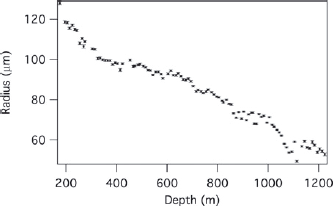
Fig. 2. Mean bubble radius as a function of depth.
4. General Trends in Bubble Number
Figure 3 shows the inverted bubble number density for all analysed samples as a function of depth. For comparison it also shows the oxygen isotope curve, the inverted dust concentration (EPICA Community Members, 2006) and two accumulation rate reconstructions (Reference RuthRuth and others, 2007; Reference Lemieux-DudonLemieux-Dudon and others, 2010) of the EDML core. Oxygen isotopes are a proxy for temperature (higher δ18O values correspond to higher temperatures). The isotope curve indicates a warm period with almost constant temperature (the Holocene) down to ~700 m (~12 ka bp), and below that the transition to the last glacial period. The dust concentration is low in the Holocene ice but rises in the glacial ice. The obtained bubble number density in the Holocene is relatively low, with averages between 300 and 400 bubbles cm−3. Below 700 m depth it quickly rises and shows a similar behaviour to the inverted isotope curve and the dust curve until ~900 m depth. Below this depth the bubble number density decreases rapidly, due to the phase transition which transforms air bubbles into air hydrates. This transformation starts slightly below 700 m depth and intensifies at greater depths. Below 1225 m all bubbles have transformed into air hydrates.

Fig. 3. Inverted bubble number density, δ18O value (EPICA Community Members, 2006), inverted dust concentration (EPICA Community Members, 2006) and accumulation rates (Reference RuthRuth and others, 2007; Reference Lemieux-DudonLemieux-Dudon and others, 2010) vs depth.
According to Reference Spencer, Alley and FitzpatrickSpencer and others (2006), the number density of bubbles formed at the firn/ice transition depends on the grain structure of the ice matrix, especially on the grain size (small grains at the firn/ice transition result in the formation of many small air bubbles, and large grains result in the formation of fewer but larger air bubbles). Further, Spencer and others argue that the grain size at the firn/ice transition is mainly controlled by the temperature and accumulation rate, in such a way that high temperatures and low accumulation rates lead to large grains, and vice versa.
Figure 3 shows that, aside from the inverted oxygen isotope curve, the dust concentration also correlates with the bubble number density. Consequently, the higher bubble number density in the Ice Age is not necessarily caused by the temperature. Experience shows that in Antarctic ice cores the concentrations of all impurities show similar behaviour with depth, in such a way that dust concentration may be used as reference for the general impurity content. The impurity concentration, which is high in the Ice Age, should have a more important influence on the grain sizes at the firn/ ice transition, and thus on the bubble number density, than the temperature. In Section 6 below, we show that the temperature has only a small influence on the bubble number density. The major reason for variations in the bubble distribution seems to be connected to the concentration of impurities (e.g. the dust or calcium concentration).
In Holocene ice we found an unexpected development of bubble number density. Between 475 m (7.2 ka bp) and 375 m depth (5.2 ka bp) the bubble number density changes by almost 25%. It increases from ~300 cm−3 within 100 m to 400 cm−3 at 375 m depth. In fact, presently the bubble number density is higher than during the Antarctic Cold Reversal (depth ~720 m, age 13 ka bp) at the end of the last glacial period, when temperature and accumulation rate are assumed to be significantly lower than now. Temperature and dust concentrations appear relatively constant over the Holocene and in particular in the mid-Holocene. To further elucidate this feature in the mid-Holocene, we show the two available reconstructions of the accumulation rate, which indicate somewhat differing accumulation histories. The accumulation rate by Reference RuthRuth and others (2007) was obtained from the depth/age relationship derived from stratigraphic matching; Reference Lemieux-DudonLemieux-Dudon and others (2010) used an inverse method to synchronize ice-core records from Antarctica and Greenland. Interestingly, both the accumulation rate given by Reference Lemieux-DudonLemieux-Dudon and others (2010) and the bubble number density begin to increase at the same depth. The simultaneous changes in accumulation rate and bubble number density above 475 m depth (7.2 ka bp) are consistent with the trend that the model of Reference Spencer, Alley and FitzpatrickSpencer and others (2006) predicts for a rising accumulation rate at constant temperature. It seems that in periods like the Holocene the bubble number density is sensitive to changes in the accumulation rate or past temperature. Furthermore, our results favour the accumulation rate of Reference Lemieux-DudonLemieux-Dudon and others (2010) as the more realistic reconstruction, assuming that the temperature reconstruction is correct. However, other explanations are also possible. We cannot exclude the possibility that the processes controlling the deposition at the surface changed at the same time and that the change in the bubble number density reflects increased katabatic winds or stormier weather in the late Holocene, compared with the early Holocene. Stronger surface winds redistribute the snow crystals over longer times, with the result that more fine-grained snow crystals are deposited. However, a change in the accumulation rate or the temperature seems to be the more attractive explanation, because the process of bubble formation at the firn/ice transition has been the subject of few detailed studies to date, and it is not known which surface features remain imprinted throughout the entire firnification, since densification is considerably affected by impurities (Reference Hörhold, Laepple, Freitag, Bigler, Fischer and KipfstuhlHörhold and others, 2012).
5. High-Resolution Stratigraphic Analysis
Our method of image analysis, i.e. the detection of all air bubbles in a section of 10 cm × 4.5 cm × 0.5 cm, allows us to investigate millimetre- to centimetre-scale variations of the bubble distribution in the ice, and to link these variations directly with the layering within the 10 cm long section. To determine the small-scale fluctuations of bubble number density and mean bubble size we calculated their running mean values, averaging over a moving window 5 mm long, through the 10 cm length of each ice sample. The results of selected samples are shown in Figure 4.

Fig. 4. Comparison of bubble number density and mean bubble radius at selected depths.
Most samples of Holocene ice have a relatively stable bubble number density (300–400 cm−3) and show only small fluctuations of about ±50 bubbles cm−3. In ice samples from the last glacial period the fluctuations are, in general, larger. Some samples have very large variations, with bubble numbers varying between 400 and >800 bubbles cm−3. Two of these samples are shown in Figure 4e and f. In most samples there exists a correlation between number density and mean size of air bubbles: the larger the number of bubbles the smaller their mean size. In glacial ice this correlation is much more pronounced than in Holocene ice. However, the obvious differences in radius (Fig. 4d–f) are hardly reflected in the size distributions (Fig. 1). The size distributions in clear- and cloudy-band ice overlap too much to exhibit these small differences in mean bubble radius (that are only 10–20 μm) between clear and cloudy bands. Curiously, at greater depths (i.e. in the middle of the bubble/ hydrate transition zone at ~1050 m depth) this correlation changes suddenly to the exact opposite: the larger the bubble number density the greater the mean size. Two samples showing this effect are depicted in Figure 4g and h.
In order to systematically analyse this correlation, and to find the depth at which this correlation inverts, we proceeded as follows: First we plotted the values of bubble number density vs the natural logarithm of the mean bubble volume for all 5 mm long windows for each sample. Then we made a linear regression and plotted the slope of each sample against depth (Fig. 5). A negative slope means that the larger the number density the lower the mean bubble size. A positive slope means that this correlation has inverted and the larger the number density the greater the mean bubble size. The plot shows that the normal correlation exists throughout the whole bubbly ice zone and in the upper part of the transition zone. This correlation is stronger in Ice Age ice than in Holocene ice. At 1050 m depth the correlation inverts abruptly.

Fig. 5. S (indicator for the correlation between bubble number density and bubble volume) vs depth. S is the slope calculated from running mean values of bubble number density and mean bubble volume fitted with a linear regression. Positive S values indicate a correlation between bubble number density and the natural logarithm of the mean bubble volume; negative values indicate an anticorrelation.
6. Impurities, Cloudy Bands and Bubble-Free Bands
The comparison of bubble number and size distribution shows that small (millimetre- to centimetre-thick) horizons of high bubble number density seem to appear preferentially in cloudy bands. Cloudy bands are ‘turbid’ ice layers, scattering the incident light due to their high content of micro-inclusions and impurities. In some deep cores they first become visible to the naked eye in the bubble/hydrate transition zone and are then the most prominent strati-graphic features in the bubble-free ice of glacial periods. In the bubbly-ice zone, cloudy bands are hardly visible to the naked eye because the strongly light-scattering bubbles conceal them. Nevertheless cloudy bands can often be made visible through special observation methods, as in the case of the microstructure mapping image of the sample from 953 m depth (Fig. 6). The comparison of Figures 4f and 6, i.e. the link between bubble distribution and the layering of the 10 cm long ice sample from 953 m depth, shows that the bubble number density is significantly increased in the dark horizons (cloudy bands). Therefore, we conclude that impurities do not only have a strong influence on the formation and distribution of air bubbles on a larger scale (Fig. 3) but also on the scale of a few centimetres. The scale of annual layers decreases on average from 4 to 2 cm between 800 and 1000 m depth (Reference RuthRuth and others, 2007). The bubble stratigraphy is also the first clear evidence for strong layering in glacial firn at the firn/ice transition. In contrast to the present opinion (Reference LandaisLandais and others, 2006), in glacial Antarctic firn the layering was much more pronounced than it is today, otherwise, the high contrast in bubble number density cannot be explained.

Fig. 6. Cloudy bands (A, B, C) visible as dark layers in the right panel (microstructure mapping mosaic) from 953 m depth. The left panel shows the high bubble number density in these layers.
Reference Hörhold, Laepple, Freitag, Bigler, Fischer and KipfstuhlHörhold and others (2012) have shown that impurities significantly influence the densification process of firn. They lead to softening and faster densification, so firn layers with high impurity concentrations reach the critical density of pore close-off first. In glacial periods the impurity concentration is increased 10–100-fold (Fig. 3). The increased impurity concentration probably slows grain growth, in particular in the layers with high impurity concentrations, the cloudy bands. At the firn/ice transition the contrast in the impurity concentration is imprinted in the grain size and thus in the number and size of bubbles. Such a process might explain the formation of many small bubbles in the cloudy bands. Because in deep firn and at the firn/ice transition the temperature is constant, neither temperature differences nor the variability of the accumulation rate on the seasonal scale can explain the observed fluctuations in the bubble number density. Therefore, the large variations in bubble number density, which we observed in ice sections from the last glacial period containing cloudy bands (Figs 4f and 6), cannot be caused by temperature or accumulation rate. Furthermore, the fact that ice layers with high bubble number density can be directly linked to impure ice layers supports the assumption that a high bubble number density is a consequence of a high impurity concentration.
As the concentration of impurities and the inverted oxygen isotope curve show similar behaviour in the EDML core, the influences of temperature and impurities on the bubble distribution on the large scale cannot be distinguished. But our results on the small scale show clearly that the influence of impurities dominates over the temperature. Therefore we conclude that the high bubble number density in glacial ice compared to Holocene ice is mainly caused by high impurity content rather than by temperature. This might also hold true for other ice cores.
In the bubble/hydrate transition zone, which in the EDML core ranges from ~700 to 1250 m depth, air bubbles transform into air hydrates. The observed inversion of the correlation between bubble number and size within the transition zone (Fig. 5) indicates that bubbles in layers with a small mean bubble size are the first to transform into air hydrates.
In the transition zone there are millimetre- to centimetre-thick layers almost free of air bubbles, called ‘bubble-free layers’ (Reference Faria, Freitag and KipfstuhlFaria and others, 2010; Reference LüthiLüthi and others, 2010). In these layers, which in the EDML core start to appear below 950 m depth, nearly all air bubbles have already transformed into air hydrates, whereas in the surrounding layers there are still many bubbles. In our results these bubble-free layers are easy to detect. Additionally, the optical observation of microstructure images, in which cloudy bands are visible as dark layers, shows that the layers almost free of bubbles can be connected to layers of high impurity content. This relationship is shown for a section from the lower transition zone (1073 m depth) in Figure 7. The bubble number and size distribution of this sample are shown in Figure 4g.

Fig. 7. Cloudy bands visible as dark layers in the right panel (microstructure mapping mosaic) from 1073 m depth. The three bands (marked A, B, C) in the left panel are characterized by complete or nearly complete absence of air bubbles.
Our results demonstrate that bubble-free layers form preferentially in impurity-rich layers that originally contained many small bubbles. The reason for an earlier transformation of bubbles in these layers might either be the smaller mean bubble radius or the high impurity content of these layers. A model of favoured hydrate nucleation in small air bubbles was proposed by Lipenkov (2000), while studies by Reference Shimada and HondohShimada and Hondoh (2004) and Reference Ohno, VYa and HondohOhno and others (2010) suggest that chemical impurities and micro-inclusions act as catalysts for the nucleation of air hydrates.
7. Conclusions
Our detailed and systematic study of air bubbles in the EDML ice core provides new information about the formation and distribution of bubbles and their relation to climate proxies. The production of high-resolution images of the ice microstructure in the field, combined with subsequent automatic image analysis, is a reasonable method for investigating bubble distributions, as the risk of relaxation effects is minimized. The high resolution gives us new information about variations in bubble number and size distribution on the seasonal and sub-seasonal scale, i.e. on the millimetre and centimetre scale, and enables us to correlate the bubble distribution to stratigraphic features visible in the ice.
We observed a bimodal bubble size distribution in shallower depths of the ice core. It is caused by two types of air bubbles: microbubbles and normal bubbles. The bubble number density on the large scale is influenced by past temperature, accumulation rate and impurity concentration, as all three parameters are intimately related. A sudden increase of the bubble number density in the middle of the otherwise climatically stable Holocene can probably be explained by a change in past temperature or accumulation rate, but not by the impurity concentration.
We found a strong correlation between number density and mean size of air bubbles, i.e. ice layers with large (small) number density of air bubbles contain small (large) bubbles. This correlation inverts in the middle of the bubble/hydrate transition zone.
Seasonal- and sub-seasonal-scale fluctuations in the bubble number density and mean bubble size are found to be larger in glacial ice than in Holocene ice. In cloudy band ice, i.e. in glacial ice, the high variability on the centimetre scale is mostly, if not completely, caused by the high seasonal variability of the impurity concentration, since firn temperature and accumulation rate cannot affect firn microstructure, and thus bubble formation mechanics, on this scale. From the observed high contrast in the bubble number density on the seasonal scale and the intimate link between impurity concentration, firn density, grain size and bubble number density we can conclude that a much stronger layering than observed in modern firn must have characterized the glacial firn in general, and in particular the firn/ice transition. Firn models need to take into account the impurity effect and the layered structure of glacial firn. Bubble number density could be included to better constrain the depth of the firn/ice transition and pore close-off.
In the lower part of the bubble/hydrate transition zone we observed bubble-free cloudy bands, indicating that bubbles in impure ice layers are the first to transform into air hydrates.
Acknowledgements
We thank D. Wagenbach for useful discussions. We also thank the Scientific Editor, Ralf Greve, and two anonymous reviewers for constructive criticism. Partial financial support is acknowledged from the Priority Program SPP-1158 of the Deutsche Forschungsgemeinschaft (DFG), grant FA 840/1. This work is a contribution to the European Project for Ice Coring in Antarctica (EPICA), a joint European Science Foundation/European Commission scientific programme, funded by the European Union (EPICA-MIS) and by national contributions from Belgium, Denmark, France, Germany, Italy, the Netherlands, Norway, Sweden, Switzerland and the United Kingdom. The main logistic support was provided by he French and Italian polar research insitutes, IPEV and PNRA, (at Dome C) and AWI (at Dronning Maud Land). This is EPICA publication No. 296.


