Introduction

The interaction between the base of the Filchner and Ronne Ice Shelves and the southern Weddell Sea is thought to be an important factor in controlling the response of the West Antarctic ice sheet to climate change (Reference ThomasThomas, 1985; Reference Budd, MacInnes, Jenssen, Smith, Veen and OerlemansBudd and others, 1987). It also provides a source of very cold water that contributes to the production of Antarctic Bottom water (Reference Seabrooke, Hufford and ElderSeabrooke and others, 1971; Reference Foldvik and GammelsrodFoldvik and Gammelsrod, 1988), a water mass which helps drive the circulation of the deep ocean (Reference Mantyla and ReidMantyla and Reid, 1983:). An understanding of the water circulation in the cavity beneath the ice shelf is prerequisite to predicting the way the interaction between the ice shelves and the ocean will change with climate.

The principal source of evidence for the oceanographic processes occurring beneath the Filchner- Ronne Ice Shelf arc conventional, shipboard hydrographic surveys just offshore from the ice front (Reference Elder and SeabrookeElder and Seabrooke, 1970; Reference Hufford and SeabrookeHufford and Sea brooke, 1970; Reference Foldvik, Gammclsrod and TorresenFoldvik and others, 1985). For the Filchner Ice Shelf, these have revealed a pattern of relatively warm water (Western Shelf Water) flowing out, and some recirculation occurring (Reference Carmack and FosterCarmack and Foster, 1975) in the Filchner Depression, a sea-floor trough beneath the ice shelf. The Ronne Depression (see Figure 1) is a corresponding; trough lying beneath the northwest sector of the Ronne Ice Shelf. The Ronne Depression is hounded by the Orville Coast on its northeastern side, a submarine ridge on its southwestern side and is generally shallower than the Filchner Depression. In January 1991, the ice shelf was penetrated at site 90/1 (77°36' S, 65°28' W) on a flowline from the Rutford lce Stream just south of the submarine 386 ridge. allowing CTD profiling, water sampling and longterm temperature monitoring. The results of this work have been discussed by Reference Nicholls, Makinson and RobinsonNicholls and others (1991) and Nicholls and Jenkins (in press).

Fig.1. Map of the southern Weddell Sea (after Reference Pozdeyev and KurininPozdyer and Kurinin, 1987), showing bathymetry in metres below sea level. The locations of the two BAS HWD sites are marked.

In January 1992, a hole was drilled at site 90/2 (76°42'S, 64°53' W) which is over the Ronne Depression, and separated from the previous site by the submarine ridge which marks the southeastern edge of the Ronne Depression. The water-column thickness above this ridge is believed to be a few tens of metres ( Reference Pozdeyev and KurininPozdyer and Kurinin, 1987), thus inhibiting exchange of water between the two sites and suggesting that the oceanographic regime at site 90/2 might be different from that found at site 90/1.

In this paper, we describe the data collected at site 90/2 and draw conclusions about oceanic processes and circulation in the Ronne Depression.

Results

A hot-water drill (HWD) (Makinson, in press) was used to create an access hole and then maintain it for 5 d. During this period, CTD profiles and water samples were collected using a miniature combined CTD sonde and water sampler. The accuracy of the CTD sensors was: ±0,1 µS m¹ (~± 0,01 practical salinity units (psu)), ±0,01°C, ±2 dbar. Before leaving the site,thermistor cables were deployed through the hole to monitor temperatures in both the water column and the overlying ice. Measurements made during the drilling gave an ice thickness of 541 m. CTD profiling showed the sea floor is at a pressure depth of 870 dbar with the ice-shelf base at 480 dbar.

The CTD profiles

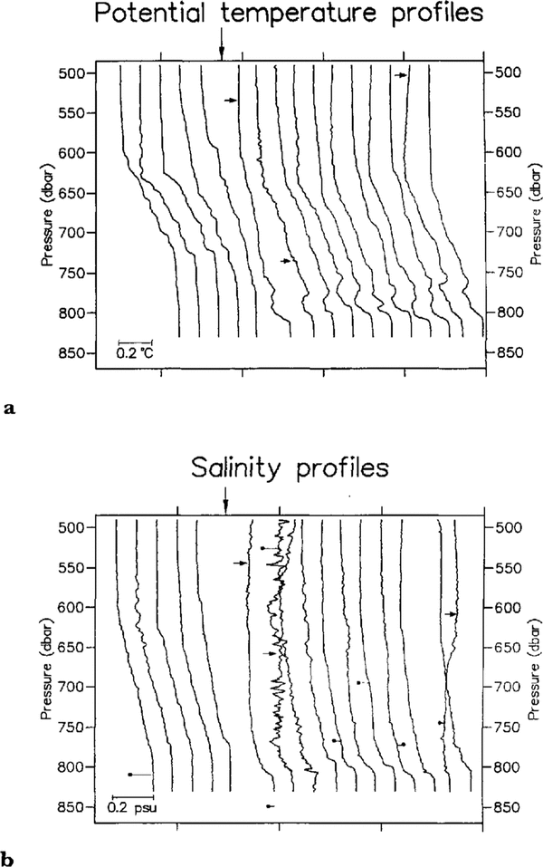
Figure 2 shows a time sequence of potential temperature (θ) and salinity (S) profiles, with the salinities of relevant water samples marked. The water column consists of two layers: a layer of Ice Shelf Water overlying a layer of Western Shelf Water. This is the first and perhaps most important result, that unmodified WSW has been found at a site 200 km from the ice front.

It is apparent that there is a change in the shape of both θ and S profiles during the sequence, with the lower layer becoming much thinner and a temperature inversion appearing above it. This change occurred during a gap in the profiling sequence caused by a break-down in the HWD system, and was used to split the profiles into two groups, called A and B. Three profiles marked with asterisks inFigure 2 were excluded from group B because of the anomalously high salinities in the upper layer of those profiles. The water-sample salinities do not agree well with the related salinity profiles. This is probably because of flushing and freezing problems with the miniature water samplers. Approximately half of the collected water-sample data was discarded because of anomalously low salinities (varying from 33 psu to 0 psu), but the remainder were within about 0,03 psu of the related salinity profiles. The specific causes are believed to be failures in the pressure-compensation mechanism of the water sampler (Reference Richards and MellingRichards and Melting, 1987) and inadequate flushing of the taps on the water sampler before decanting the sample, allowing contamination of some samples with fresh water from the borehole. Other groups have experienced lack of agreement between the salinity of water samples and CTD measurements from beneath ice shelves (Reference FosterFoster, 1983) and in particular with this type of water sampler (personal communication from E. Fahrbach). As a consequence, we do not place much reliance on the water-sample salinity data.

Fig.2. Sequence of potential temperature and salinity profiles, showing how the structure of the water column changed over the 5d the HWD hole was open. The sequence is not linear in time, and the large arrow marks a 2d period in which no profiling occurred. Profiles were split into two groups A and B (see text) Which are separated by the 2d gap), Profiles to the right of the arrow were measured on the final day of profiling. The three profiles indicated with small arrows were excluded .From group R because of anamalously high salinities at the top of the water column. a. Temperature profiles: profiles are consecutively shifted +O,12°C to the right. b. Salinity profiles: profiles are consecutively shifted + 0,1 psu to the right. Dots mark water-sample salinities with lines attaching them to the relevant profile. The water-sample salinities have been shifted by the same amount as the related profile.

Figure 3 (8#x007E;S plot with depths marked on the profiles) is a θ-S plot of the means of the profiles composing groups A and B. It highlights the different θ-S characteristics of the two groups of profiles. Group B has a slightly fresher and colder WSW lower layer and a slightly colder ISW upper layer than group A. The main difference in the shapes of the group 13 and group A profiles may be explained either as the intrusion of a colder water mass just above the WSW or as the replacement of the WSW in group A with a colder, fresher and thinner layer of WSW. The latter explanation would suggest that the temperature inversion in group B is a transitory feature.

Figure 3 Mean profiles of potential temperature and salinity for groups A and B (see Figure 2).Lines on the lefthand side are potential temperature (θ) and those on the righthand side are salinity. In both cases, group A profiles are indicated by the bold lines.

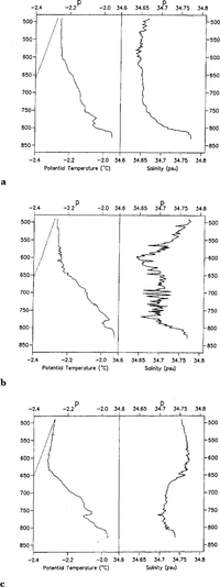
The “unstable” profiles

The three profiles excluded from group B are shown in more detail inFigure 4. They are all characterized by anomalously high salinities and temperature inversions in the upper layer. The salinities shown in Figure 4b and Figure 4c are as high as those in the lower (WSW) layer, giving a large density inversion which should cause the water column to overturn vigorously. The result of such overturning would be a homogenized water column which, as can be seen from Figure 2, does not happen. Because overturning has not occurred, the density inversion, implied by the CTD data, cannot be real. Two possible explanations for this are that the conductivity cell on the CTD probe has produced erroneous data or there is a suspension of ice crystals present in the water column. A mechanism by which the conductivity cell can read high is not obvious, since contamination of the cell usually leads to a reduction in measured conductivity. In addition, the data show no evidence of electronic problems in the probe. The latter explanation, that there is a suspension of ice crystals in the water column, does not fit the data well either, since the temperature on all three profiles is between 0,01° and 0,1°C above the in situ freezing point, and the presence of ice crystals in thermal equilibrium would lead to the water being at the in situ freezing point. If we consider the group B mean temperature profile and the in situ freezing-point profile, we find that the temperature profile ofFigure 4c bisects them, indicating that theFigure 4ctemperature profile would be produced by mixing constant proportions (with depth) of group B ISW with water at the appropriate pressure-freezing point. This hypothesized water mass with a temperature at the freezing point, which we will call cold ISW. could contain frazil ice (Reference Foldvik and KvingeFoldvik and Kvinge, 1974). with this interpretation, the presence of ice crystals in the water column results from advection and mixing between two different ISW masses, in one of which ice crystals have formed. Because of the difference between turbulent and molecular thermal diffusivities. the ice crystals have not yet melted, i.e. the proportion of ice crystals in the water column beneath this site is controlled by turbulent diffusion and advection between cold ISW and group B ISW, but the time-scale for them to melt in the new composite water mass is controlled by the molecular diffusion of heat. Order-of-magnitude calculations indicate that at the bottom of the salinity inversions (˜600 dbar onFigure 4bandFigure 4c) ice crystals will melt in a time-scale of the order of seconds, while near the ice-shelf base the time-scale will be of the order of minutes. Looking at the profiles in the context of these time-scales, it would appear that: in Figure 4cadvection has only just ceased or is still occurring and that melt is occurring mainly at the lower edge of the intrusion; in Figure 4b advection has ceased and ice crystals are in the process of melting; in Figure 4a the water column above the lower layer is approximately isohaline, indicating that melt would have been going on for several minutes, removing ice from all but the very top of the water column. The noise on the salinity records may be explained in the upper layer by the melting of ice crystals, and below the salinity inversion by the turbulent overturning of water which the ice crystals have risen above, removing the stabilizing effect of their buoyancy. This may also explain why the salinity in the lower layer ofFigure 4c is reduced, though the limited data prevent a comprehensive explanation of such a complicated process.

Since the profile inFigure 4c appears to show the most recent signs of advection, we can try to calculate the proportion of ice that would be required to stabilize the salinity inversion. Assuming the composite water mass has a bulk-density profile less than or equal to the average profile for group B, because overturning does not take place, the proportion of ice crystals must be-greater than 1,2%by volume. Using the salinity of the water below the salinity inversion as a bulk salinity gives proportions of ice crystals of 1,6 and 2%,respectively, for Figure 4candFigure 4b,though this will have been increased if mixing with water from the pycnocline has occurred. If we then assume that ice crystals mix in the same way as heat, and that cold ISW is at the in situ freezing point, the concentration of ice crystals in cold ISW would have been greater than 3% by volume,

Fig.4. θ and S profiles of the three excluded profiles, with the in situ freezing point marked by the dotted tine

The thermistor cable temperature record

Immediately after the deployment of the thermistor cable, it was logged for 2d at 5 min intervals before being left for the winter with a logging interval of 30 min. The 2 d record is shown inFigure 5.The variations in temperature of each thermistor indicate that the cable is swinging in the tidal currents with the thermistors passing up and down through the water column. Simple hydrodynamic modelling (e.g. Reference Steele and MorisonSteele and Morrison, 1992) of the cable's behaviour suggests that the currents have maximum speeds of around 0,5 ms¹ and minimum speeds of under 0,1 ms¹, assuming no variation in velocity through the water column, These values are in broad agreement with velocities measured at the ice front (Reference Gammelsrod and SlotsvikGammelsrod and Slotsvik, 1981). The record also demonstrates the occasional presence of a colder water mass, when the temperature of the whole water column drops, and the upper layer reaches temperatures lower than seen in the CTD profiles, Figure 5 shows the recovery from one such “cold event” takes 2–3 h.

Fig.5. 2d section of the thermistor cable record. The record starts 4h after the final CTD profile Figure 2.Temperatures were logged at 5min intervals, Each solid line represents the record from one of the ten thermistors, which were evenly spaced at 35 m intervals down the cable, starting 40 m below the ice-shelf base. Dashed lines mark times when the cable is believed to be hanging vertically in the water column

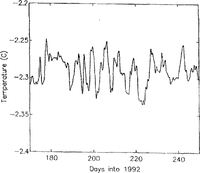
Figure 6shows that “cold events” occur with a period of about 100 h. The only similar behaviour seen in the CTD profiles is from the three temperature profiles in Figure 4,which are depressed by ~0,01–0,02°C below the mean profile, over the whole water column.

Fig.6. 70 d temperature record from the uppermost thermistor, with a logging interval of 80 min, The record has been low-pass filtered with a cut-off of 24 h to remove any tidal signal

Discussion

The most general result from this work has been the observation of unmodified WSW below the ice shelf at a considerable distance from the ice front. The idea of shelf water flowing underneath the ice shelf was originally postulated by Reference Seabrooke, Hufford and ElderSeabrooke and others (1971) and expanded upon by Reference Jacobs, Gordon and ArdaiJacobs and others (1979).

In addition, the data show that the water column exists in two different conditions, as defined by groups A and B above. This is seen on both the CTD data and the thermistor record: 8 h before the deployment of the thermistor cable, the CTD profiles indicate that the characteristics of the water column fall within group B. The short thermistor record shows that temperature of the water column is initially colder, with upper-layer temperatures of about -2,30°C. Temperatures this low were only seen on the three profiles excluded from group B. After a day of monitoring, the temperature of the upper layer increased to 2,24°C. This is larger than the temperature difference between the two groups of CTD profiles. However, a slight cooling trend can be seen on the first day of the short record (Figure 5), and the longer record (Figure 6) shows that the changes from colder water to warmer water are not necessarily the same size.

The longer thermistor record (Figure 6) shows that periodically the temperature of the upper layer drops to temperatures significantly lower than group A or B. Similar behaviour is seen on three CTD profiles which suggest that the water column may contain ice crystals in suspension. The periodic appearance of low temperatures indicates that a mechanism exists which can advect water across the Ronne Depression and that this mechanism is not tidal. The geometry of the Ronne Depression suggests that this cold water originates from northeast of site 90/2. The existence of marine ice at the base of the ice shelf adjacent to the Orville Coast may indicate that cold ISW comes from that side of the depression.

Conclusions

The work at this site has revealed a water column consisting of lSW overlying unmodified WSW, with tidal currents which are strong compared with site 90/1 where there was little indication of tidal motion (Reference Nicholls, Makinson and RobinsonNicholls and others, 1991). The water column exists in more than one state, with changes in the thickness and properties of the ISW and WSW layers being observed. The advection of a cold water mass containing ice crystals in suspension is suggested by three CTD profiles, and this is consistent with the thermistor-cable record in which periodic drops in the temperature of the water column can be seen. This cold, ice-bearing water mass is suggested to be located on the northeastern (Orville Coast) side of the Ronne Depression.

Acknowledgements

The authors express their gratitude to the British Antarctic Survey's field operations staff and Air Unit, and especially to J. Sweeney and S. Davis for their assistance at the drill site.