


1. Introduction
Calving is one of the most important sources of ice lost by tidewater glaciers, together with surface, basal and submarine melting. For all glaciers on Earth, surface accumulation adds about 3000 × 1012 kg water equivalent annually, while surface ablation removes about 1000 x1012kg and calving of icebergs about 2400 x1012kg (Reference HoughtonHoughton and others, 2001). Despite their importance, calving and associated dynamic changes are some of the least understood glacial processes and remain a key uncertainty in the future evolution of tidewater glaciers.
Data of temporal variation of calving events and velocities directly from the calving fronts are very valuable because they provide information about calving processes. However, such data are rare due to the dangers and difficulties connected with making the measurements. Studies like remote sensing can inform about the seasonality of calving; however, to learn about the details of calving processes, calving events must be observed in detail. Such detailed observations enable the understanding of what controls calving and what triggers individual calving events.
The following techniques have been used previously to capture the nature of the calving processes: direct visual observations (Reference Warren, Glasser, Harrison, Winchester, Kerr and RiveraWarren and others, 1995; Reference O’Neel, Echelmeyer and MotykaO’Neel and others, 2003, Reference O’Neel, Marshall, McNamara and Pfeffer2007), passive seismic (Reference QamarQamar, 1988; Reference O’Neel, Echelmeyer and MotykaO’Neel and others, 2003; Reference Amundson, Truffer, Lüthi, Fahnestock, West and MotykaAmundson and others, 2008) and ground-based interferometric radar (Reference Rolstad and NorlandRolstad and Norland, 2009). Direct visual observations produce very detailed data about calving of icebergs, giving information about the timing, location and style of calving. However, this method requires a permanent presence in the field and the results can be altered by bad visibility (darkness, fog), difficult conditions for observations (storm, rain, wind) or lack of attention from the observers. Passive seismic is a good technique to obtain calving-event frequency and possibly location, independently of weather conditions. However, uncertainty remains over the origin of icequakes and the fact that some of them are not caused by calving of icebergs but by fractures in the glacier body or icebergs rolling in the fjord (Reference Amundson, Truffer, Lüthi, Fahnestock, West and MotykaAmundson and others, 2008). Recently, ground-based radar has proved to be valuable for measuring ice-front velocity and identifying calving events of Kronebreen (Reference Rolstad and NorlandRolstad and Norland, 2009). However, what was absent in that study was spatial information about the returned radar signal. They also showed that identification of calving events was possible on the backscatter amplitude plot, but made no attempt to extract calving-event frequency automatically from the dataset. The use of ground-based radar is appealing because it can be conducted at a safe distance from the glacier front and it produces both good spatial and temporal resolution. It can be operated automatically and does not require a constant presence in the field. This last characteristic offers a big advantage compared with direct visual observations, which also provide good spatial and temporal resolution but require a constant presence in the field. Finally, the topography in front of Kronebreen offers an ideal setting for radar studies: a lateral moraine providing a direct line of view to the glacier front (Fig. 1).

Fig. 1. Orthorectified aerial photograph of Kronebreen in 1990 (Norwegian Polar Institute). The white triangle marks the position of the ground-based radar, the circle marks the position of the camp from where the direct visual observations were performed and the two squares mark the position of the cameras, the solid square showing the position of the single-imaging camera. Red triangles mark the positions of control points. The white and red rectangles define the five different areas used for the direct observations.
During the field campaign in August 2008 we observed the calving front of Kronebreen visually during the same period as the radar campaign was conducted and we collected photogrammetrical data. We wanted to investigate whether we could detect all calving events with the radar and, if not, which calving events can be detected. In this paper we demonstrate spatial interpretation of a radar backscatter signal with the help of photogrammetry. We also present a new technique to detect calving events automatically using image-processing change detection applied to radar backscatter data. We establish a time series of calving events using this algorithm and compare the results with registered visual observation of calving events. Finally, we look at the temporal geometrical evolution of the calving front.
2. Field Area
Kronebreen is a grounded polythermal tidewater glacier located ∼14km southeast of Ny-Alesund, western Spitsbergen. The glacier drains a glacial basin called Holtedahl-fonna, which covers 700 km2 and is ∼ 3 0 km long. The lower 18 km of the glacier are heavily crevassed. The terminal ice cliff had an elevation ranging from 5 to 60 m above the fjord surface at the end of August 2008. The height of the front experiences numerous variations during the year. The lowest portion in August 2008 ∼500m long) reached only 5 m above the water, but had been standing at 40 m above the water in May 2008. This variation between two months indicates a very active glacier front
3. Methods
To test this new technique of calving-event detection on Kronebreen, we used a ground-based radar from 26 to 30 August 2008. To validate the results, terrestrial photogrammetry and direct visual observations were performed during the same period. We chose to use a ground-based radar to collect data from the glacier front because it provides a continuous dataset about the glacier-front movement and the range to the front yielding the calving events.
Terrestrial photogrammetry gives good data about the front position and shape as well, but there is a trade-off between spatial and temporal resolution which does not exist with the radar. In fact, terrestrial photogrammetry at Kronebreen does not provide a spatial accuracy better than 1 m; however, it is a very good technique to image the front shape.
3.1. Ground-based radar
We used a 5.75 GHz, frequency-modulated continuous-wave (FM-CW) radar located about 4 km west of the glacier front (Fig. 1). The range resolution was 1 m and the measurement interval was 0.5 s. The antenna lobe had an opening of 9°, which covered about 645 m of the 3500 m of the entire ice-front width. In this paper, we define the dimensions as follows: width is the distance along the ice front, height is the vertical distance above the waterline and depth is the up-glacier distance between the ice front and the calving fracture. A corner reflector was placed between the radar antenna and the glacier for calibration. The radar was running continuously for approximately 116 hours between 26 and 30 August 2008.
A technique used to obtain the range variation of natural scatterers on the glacier front for velocity measurements is described by Reference Rolstad and NorlandRolstad and Norland (2009). In their paper, the relative velocities were determined interferometrically from the change in phase between two consecutive samples. In this paper, we have used only the amplitude of the backscattered signal in conjunction with optical methods to identify calving events and automate the process of this identification.
The radar can be left to run automatically. A similar permanent installation for mountain rockslide monitoring in the Norwegian fjord Tafjorden has run since 2006 (Reference NorlandNorland, 2006). The power consumption is similar to a personal computer’s (400–800 W), and the antenna output power is 0.001 W. The data storage capacity can be designed to fit the requirements for different monitoring durations. The system is very stable in our experience and, if installed correctly, there is no need to check the installation. Antennae may be protected with a radome, and for permanent monitoring the radar may be placed in a house. This system could thus be used for a future campaign that would cover a much longer time span.
3.2. Interpreting a radar backscatter amplitude plot of a glacier front
In order to interpret both spatial and temporal variations in the signal, it is necessary to understand what can affect the radar backscatter in theory. Five main factors can affect the radar backscatter signal: incidence angle, the frequency and polarization of the radar, surface roughness, and moisture.
The incidence angle plays the largest role in our study because it changes dramatically as the terminus geometry changes. The incidence angle is the angle between the normal to the object surface (calving front in our case) and the direction of the incident radiation. The smaller the incidence angle, the stronger the backscatter amplitude. In our case, the incident angle is very large over the intervening water (almost 90˚) and becomes close to 0˚ when the radar beam intercepts the glacier front. This abrupt change in the incidence angle accounts for the overall patterns of spatial variations on the radar backscatter amplitude plot.
The frequency and polarization of the radar were kept constant during the week of investigation, so the observed temporal changes in the backscatter values were mainly caused by temporal variations of the object surface properties and not the radar properties. Tests were conducted with different antenna configurations in 2007, yielding similar backscatter intensity for all polarizations (Reference Rolstad and NorlandRolstad and Norland, 2009).
Roughness influences the interaction of the radar signal with the ice surface and is a function of the incidence angle and the wavelength. The rougher the surface, the stronger the backscatter amplitude. In our case, the object surface is considered rough if the mean height of surface variations is >0.02 mm, which is the case for the glacier surface. We can assume that the surface stays rough throughout the observation period.
Moisture has a strong impact on the surface reflectivity, which increases with the moisture content, so changes in moisture caused by rainfall or surface melting might induce some changes in the backscatter intensity. However, the overall intensity was relatively constant during the measurement campaign. Hence we conclude that moisture variations have little effect on our dataset.
The propagation velocity of an electromagnetic wave in air varies with the refractive index, and the calculated range will vary accordingly. The refractive index varies with the meteorological parameters: temperature, pressure and humidity. Variations in range due to this effect can be eliminated using measurements from a stable corner reflector (Reference NorlandNorland, 2006) near the glacier or by estimating the variations of the refractive index using local meteorological data (Reference NorlandNorland, 2007). However, experience shows that these variations in measured range are small and gradual. Variation in measured distance, mainly due to changes in the refractive index, over a distance of 2900 m was 30 cm during two winter months in Tafjorden (Reference NorlandNorland, 2006). We therefore assume that the ranges in the backscatter amplitude plot from Kronebreen vary by <10 cm due to refractive index uncertainties during the 116 hours of measurements in 2008.
Destructive interference due to multipath scattering of the electromagnetic wave and the tidal cycles may lead to a periodic pattern of zero intensity at specific ranges in the amplitude of the backscatter plot. This geometrical phenomenon is described in Reference Rolstad, Chapuis and NorlandRolstad and others (2009) and it has no influence on the results described in this paper
3.2.1. Natural permanent scatterers on the glacier surface
A permanent scatterer on the glacier surface moves towards the radar and reflects the signal back to it. On a backscatter amplitude plot this is displayed as a permanent feature the range of which decreases with time, as the permanent scatterer moves closer to the radar (Fig. 2).
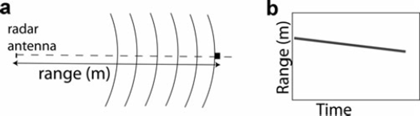
Fig. 2. (a) Schematic aerial view of a natural permanent scattering reflector (black square) moving towards the radar antennae at constant speed. The distance between the radar and the reflector is called the range. (b) Resulting backscatter amplitude plot.
3.2.2. Spatial configuration of the glacier front
The shape of the front and its spatial arrangement with respect to the radar is important to interpret correctly the radar backscatter amplitude plot. Figure 3 presents three different spatial configurations of a radar illuminating a glacier front. To simplify we only show radar beams one range-unit apart. Each electromagnetic wave associated with a single range value can intersect the glacier front once or twice, depending upon the spatial configuration. Thus different configurations can produce similar amplitude plots, as shown in Figure 3. In order to determine how the radar beam interacts with the front and where the backscatter comes from, it is necessary to know the spatial configuration of the radar and the glacier front. In this study, we determined this configuration by the use of photogrammetry.

Fig. 3. (a–c) Glacier fronts (typical selected examples), moving towards the radar at constant speed, and radar beams one range-unit apart; and (d) corresponding backscatter amplitude plots.
3.2.3. Geometry of vertical ice features acting as reflectors
Vertical ice features act as reflectors and form bands of high intensity in the amplitude backscatter plot (Fig. 3d). A glacier front that is a vertical cliff will produce a narrow band in the plot, whereas a front displaying a stepped shape will produce a wider band. This geometry is illustrated in Figure 4. We can easily estimate s, the horizontal distance between the bottom and the top of the glacier front, from how wide the high-amplitude band is on the amplitude plot (r 2–r 1).

Fig. 4. Geometry of the stepped shape of the front.
3.3. Terrestrial photogrammetry
Terrestrial photogrammetry is used here to obtain the shape of the glacier front at the time when the radar campaign was conducted. It is a method for measuring object sizes and shapes using photographs taken from the ground. In this study we have used monophotogrammetry, analysing single images to obtain two-dimensional measurements, and stereophotogrammetry, using pairs of images to derive the three dimensions of the object. Photographs were taken with a Nikon D40 digital camera. Seven control points were placed on the shore and on nearby mountain peaks (Fig. 1). Because stereophotogrammetry is a more complex procedure, we retrieved the three-dimensional measurements of the glacier front from one stereo-pair of clear and sharp images photographed in clear weather on 29 August 2008. Fluctuations in front position were documented from single images using monophotogrammetry, which provides less accurate measurements, but can be performed faster and does not require very sharp images.
3.3.1. Monophotogrammetry
The camera position was about 1.5 km west of the front (Fig. 1). Images were taken on 28, 29 and 31 August 2008. The front position is seen as the intersection between the plane defined by the fjord surface and the glacier ice cliff. A monophotogrammetric routine allowed the determination of the coordinates of this intersection line. This routine was developed by M. Truffer at the University of Alaska Fairbanks, based on Reference Krimmel and RasmussenKrimmel and Rasmussen (1986), and further improved by O’Neel in 2009. Several studies (e.g. Reference Motyka, Hunter, Echelmeyer and ConnorMotyka and others, 2003; Reference O’Neel, Echelmeyer and MotykaO’Neel and others, 2003, Reference O’Neel, Pfeffer, Krimmel and Meier2005) have applied this routine successfully to document the fluctuations of glacier fronts. We measured the camera position, elevation and pointing angles, and used two ground-control points. Tidal amplitude and timing in the fjord are required and were obtained from the Norwegian Mapping Authority. The spatial resolution of the monophotogrammetry is about 3 m.
3.3.2. Stereophotogrammetry
Stereophotogrammetry uses two simultaneous images of the same object to reconstruct its three dimensions. We applied it here to obtain a precise map of the front topography: shape, height and width. The cameras were located about 1.5 km west of the front, on a side moraine (Fig. 1), and the distance between the two cameras was 309 m. The requirements for the stereophotogrammetrical method are the known positions and elevations of the two cameras and the presence of at least six control points in the field of view of the camera (Fig. 1).
Image analysis included camera calibration, relative and absolute orientation, stereo-resampling and measurements. The purpose of the calibration was to estimate the optical properties of the camera: focal length, distortion parameters and the point of best symmetry. The horizontal accuracies were obtained by comparing the position of known objects to their estimated position using stereophotogrammetry. At the ice front, the accuracy varies from 5 to 45 m. The accuracy decreases as the object gets further from the cameras; it fluctuates from 0.5 to >200m at 8 km from the camera. The vertical accuracy (-1 m) was estimated by comparing the front heights obtained on three different stereo-pairs.
3.4. Direct visual observations
Direct visual observations consisted of identifying and registering calving events from a safe distance. Between 26 August and 1 September 2008 we continuously observed the front activity of Kronebreen at about 1.5 km west of the fronton a lateral moraine (Fig. 1). Four people were involved with the observations. We recorded the timing, location, type and magnitude of the events. The timing was determined with an accuracy of 1 min. To define the location, we divided the glacier front into five different areas (Fig. 1). Six different types of event were observed: avalanche of ice when the pieces were too small to be identified as blocks; block slumps when a block of ice was disintegrated from the front; column drop when a column of ice collapsed vertically or quasi-vertically; column rotation when a column of ice collapsed with a rotation movement; submarine when a block of ice was released from underwater; and internal when we could only hear a loud crack, assuming fracturing of ice not associated with calving of icebergs or any missed/out-of-view calving events. The magnitude was attributed subjectively for each event, based on a combination of the volume of ice involved, the width of the glacier affected and the duration of the event. We used a magnitude scale (Reference O’Neel, Marshall, McNamara and PfefferO’Neel and others, 2007) which ranged from 1 to 20, 20 being the whole front collapsing. The subjectivity led to a discrepancy of ± 1 in the magnitude estimation from one person to another.
4. Results and Discussion
In this section we present the three main results obtained by analysing the radar signal in combination with photogram- metry and visual observations. This yields a more complete interpretation of the radar plot linked to the glacier-front geometry, an automatic way to detect individual calving events through image-processing change-detection techniques, and a temporal interpretation of the variations of the front positions.
4.1. Glacier front topography from photogrammetry
The stereophotogrammetry shows that the front is about 50 m high at the place on the glacier where the beam centre intercepts the front (Fig. 5). For the rest of this study we call this location beam centre (BC). The front at this particular area of the glacier is not vertical but presents a stepped shape (Figs 4 and 5). At BC the front reaches its maximum height 15–20 m up-glacier from the actual terminus position.
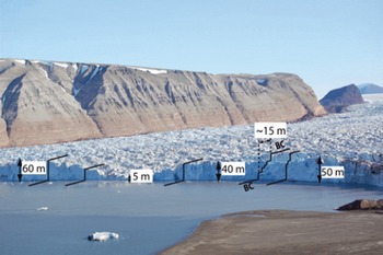
Fig. 5. Photograph of the calving front on 29 August 2008. The black lines indicate the front topography. BC marks the intersection of the radar beam centre with the front.
4.2. Interpretation of the radar backscatter amplitude plot
Figure 6 shows the radar backscatter intensity in the radar range (3900–4500 m) between 12:00 universal metric time (UMT) on 26 August and 08:00 UMT on 30 August. In general we see strong backscattered signals due to small incident angle and vertical ice walls. When these strong signals form continuous ‘lines’ in the backscatter amplitude plot, with a trend representing a reasonable glacier velocity, we can assume that they are from vertical features of the moving glacier. We then used photogrammetry to determine one or several possible reflection points on the glacier corresponding to the measured range.
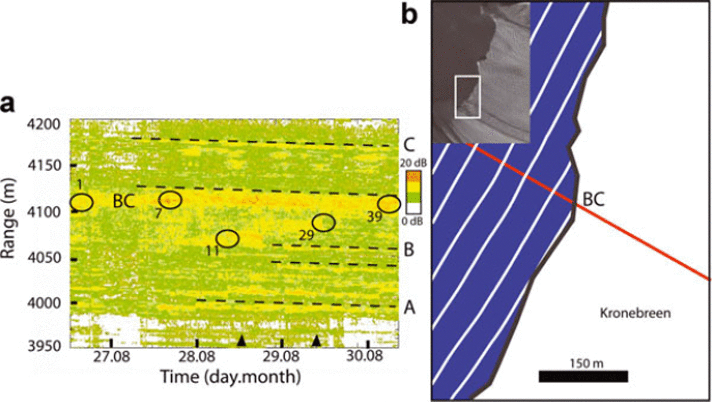
Fig. 6. (a) Radar backscatter intensity (dB). The vertical glacier front ranges from 3950 to 4200 m. Measurements were conducted from local time 12:00 on 26 August to 08:00 on 30 August 2008. Black circles indicate sharp retreats of the front, representing the five calving events discussed in section 4.3. Dashed lines indicate strong permanent backscatter features. The two black triangles mark the time at which mono-photographs were taken. (b) Calving front as imaged by Système Probatoire pour l’Observation de la Terre (SPOT) on 1 September 2007. Spirit Program © Centre National d’Etudes, France (CNES), 2008, 2009 and SPOT Images_2007 (all rights reserved). The red line marks the radar beam centre, and the white arcs illustrate the radar waves hitting the glacier front.
The range to the glacier front lies between 3950 and 4200 m. Beyond 4150 m, there is a periodical pattern of destructive interference resulting from multipath scattering due to radar glacier geometry and tidal cycles (Reference Rolstad, Chapuis and NorlandRolstad and others, 2009). The strongest and most permanent feature lies in the range 4100–4120m. This is BC, the intersection of the centre beam of the radar with the calving front (Fig. 6b). Overall, this feature is advancing during the observation period with some sharp retreats corresponding to calving events (Fig. 6a) which are discussed in section 4.3. Results from the stereophotogrammetry showed that the geometry of the front and the relative position of the radar are such that each transmitted electromagnetic wavefront intercepts the glacier front only once. Any high reflecting features in the amplitude plot that appear closer than BC are parts of the glacier front located on the right-hand side of BC looking down-glacier, or an iceberg in front of the glacier, whereas any features that appear further away than BC on the amplitude plot are physically parts of the glacier front on the left-hand side of BC looking down-glacier. The topographical height of the ice feature of high-intensity backscatter at range 4120m is about 20–25m. Given the width of the high-amplitude band at BC on the amplitude plot, we deduce that the front has a stepped shape. Photographs (Fig. 5) confirm this radar observation.
4.3. Detection of calving events
Black circles on the backscatter amplitude plot of Figure 6a indicate sharp retreats at different places on the ice front at different times. Each of these is shown in more detail in Figure 7. We applied an automated change-detection algorithm on the backscatter data to build a calving-event time series. The algorithm compared a 30 s averaged backscatter value at time t=t 0 with another at time t=t 0+60s, at the same range. We set a change threshold of 5 dB. If the change in the backscatter value was below this threshold, we interpreted no change in the front geometry. However, if the change in the backscatter value was larger than the threshold, we took this to indicate a change in the front geometry, and its intensity was indicated by the colour scale ranging from green (small changes) to red (large changes). Figure 7 shows the result of this change-detection algorithm.

Fig. 7. Change-detection plot showing the time and place where column drops and column rotations were detected by the radar during –116 hours. Vertical dashed lines mark the events observed visually that were successfully identified automatically in the radar data by the change-detection routine. Dots below the plot mark observed events that were not detected. The upper part of the plot shows examples of five events (ID 1, 7, 11, 29 and 39) identified in the raw backscatter radar data. The bold lines mark the corresponding interpreted retreat of the front.
To validate the method, we compared the result of this radar backscatter change detection with direct visual observations for the whole 116 hour period. All column-drop and column-rotation events that occurred within the radar beam (southernmost side of the front) during the measurement period are plotted on the change-detection plot (Fig. 7).
There is a good overall agreement between the observed calving events and those detected using the radar change-detection algorithm. Out of 41 events in total, 35 were identified with the radar (85%). Filtering out the events with a magnitude smaller than 2 (leaving 33 events), the percentage of identified calving events reached 92%. Almost all column-drop and column-rotation events with a magnitude larger than 2 that occurred within the radar beam were identified using the change-detection algorithm on the backscatter data.
The observed calving events that were not identified using the algorithm, and thus not seen on the change-detection plot (black squares below the plot), could be out of the radar range because the area covered by visual observations was larger than that covered by the radar. Conversely, changes automatically identified and displayed on the radar plot which do not appear in the visual observations list could have been missed by the observer for a number of reasons: lack of attention or bad visibility such as foggy conditions. Moreover, a block that rotates but does not calve within the time window of 60 s during which the backscatter values are compared may still modify its incident angle, thus leading to a changed backscatter value even though no calving occurred. Icebergs floating in front of the glacier can also lead to changes in the backscatter value. This can be an issue in our case because icebergs can be in the way between the radar and the glacier front.
4.4. Temporal evolution of the calving front
Permanent strong backscatter features show the variations in front position at different places across the front. We followed several strong backscatter features on the radar plot (Fig. 6a) to obtain the change of the front position or velocity during the observation period. Monophotogram-metry was performed during the same period, with two images taken during the time the radar was operated (black triangles in Fig. 6a).
Figure 8 represents the variation of the front position dL between 28 and 29 August for the area of the front covered by the radar. We observe an overall good agreement between the change in front position obtained by photogrammetry and that from tracking different parts of the front on the radar signal. However, the front at BC shows a different behaviour on the radar data and on the photogrammetry data. On the radar data the front shows constant velocity and hence an advancing front at BC, whereas the photographs suggest no net change or a slight retreat over the period. We cannot explain this discrepancy. The other locations (A, B and C) show better agreement between the radar and photographic data. The fact that we observe almost no change in the front position at BC means that the calving events at this location have been neutralizing the general advance of the front, leading to a quasi-non-change in dL On both sides of BC, the front has been advancing on average, as shown in Figure 8, indicating that calving activity was not large enough to counterbalance the advance caused by glacier flow.
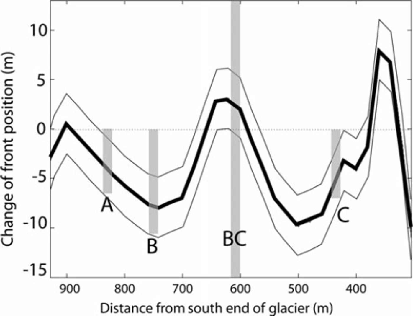
Fig. 8. Variation of the front position along the glacier front (thick curve) determined from monophotogrammetry, looking up-glacier. Positive change in the front position is retreat. The two thinner lines indicate the estimated accuracy of the measurements. A, B, BC and C mark the positions of the features identified on the radar amplitude plot in Figure 6a.
5. Conclusions
Ground-based radar is a powerful technique with great potential to investigate the behaviour of a calving front. It presents the advantages of being conducted at a safe distance from the front and not requiring a permanent presence of personnel in the field. Moreover, coupled to terrestrial photogrammetry, it can provide very accurate data on the calving-front behaviour, both spatially and temporally. We have presented here the results of 1 week of radar data from the front of Kronebreen, coupled with terrestrial photogrammetry and direct observations. The main results are that:
it is possible to determine the calving-event frequency using a change-detection algorithm on ground-based radar data;
the majority (92%) of column drops and column-rotation events with an estimated magnitude larger than 2 ∼1000m3) can be detected;
terrestrial photogrammetry provides necessary information to interpret spatially the radar backscatter signal.
Acknowledgements
The work is part of the International Polar Year project GLACIODYN funded by the Norwegian Research Council. The fieldwork was supported by Svalbard Science Forum. We thank S. O’Neel for his help with monophotogrammetry analysis and A. Burras and N. Peters for their help in the field. Comments from reviewer J. Amundson, an anonymous reviewer and A. Smith greatly improved the manuscript.


