Case Report
Using Mathematical Procedure to Compute the Attenuation Coefficient in Spectrometry Field

Mohamed Elsafi1, Mona. M. Gouda1, Mohamed. S. Badawi1,2*, Abouzeid. A. Thabet4, Ahmed. M. El Khatib1, Mahmoud. I. Abbas1 and Kholud. S. Almugren4
1Physics Department, Faculty of Science, Alexandria University, 21511 Alexandria, Egypt
2Department of Physics, Faculty of Science, Beirut Arab University, Beirut, Lebanon
3Department of Medical Equipment Technology, Faculty of Allied Medical Sciences, Pharos University in Alexandria, Alexandria, Egypt
4Physics Department, Faculty of Science, Princess Nourah Bint Abdulrahaman University, 11544-55532 Riyadh, Saudi Arabia
*Address for Correspondence: Mohamed S Badawi, Physics Department, Faculty of Science, Alexandria University, 21511 Alexandria, Egypt, Tel: +201005154976; Email: ms241178@hotmail.com
Dates: Submitted: 19 December 2016; Approved: 03 February 2017; Published: 06 February 2017
How to cite this article: Elsafi M, Gouda MM, Badawi MS, Thabet AA, El-Khatib AM, et al. Using Mathematical Procedure to Compute the Attenuation Coefficient in Spectrometry Field. J Radiol Oncol. 2017; 1: 022-030. DOI: 10.29328/journal.jro.1001003
Copyright License: 2017 Elsafi M, et al. This is an open access article distributed under the Creative Commons Attribution License, which permits unrestricted use, distribution, and reproduction in any medium, provided the original work is properly cited
Keywords: Gamma-ray spectrometry; Linear attenuation coefficient; Effective solid angle; Average path length; Mathematical method

ABSTRACT
In gamma-ray spectrometry, the analysis of the environmental radioactivity samples (soil, sediment and ash of a living organism) needs to know the linear attenuation coefficient of the sample matrix. This coefficient is required to calculate the self-absorption correction factor through the sample bulk. In addition, these parameters are very important because the unidentified samples can be different in the composition and density from the reference liquid sources which are usually used for efficiency calibration in the radioactive monitoring process. The present work is essentially concerned to introduce a mathematical method to calculate the linear attenuation coefficient without using any collimator. This method was based mainly on the calculations of the effective solid angle subtended by the source-to-the detector configurations, the efficiency transfer technique and the average path lengths through the samples itself. The method can be used as a tool for the calculation of the linear attenuation coefficient of unidentified materials with good facility to use it in the calibration process of γ-ray detectors, particularly in the study of soil samples. The results are compared with the data from NIST-XCOM to show how much the results are in close agreement and to give the validity of the approach.
INTRODUCTION
Relative measurement for the radioactivity analysis of environmental samples can be used as a typical technique of gamma-ray spectrometry. It is adopted to measure the radioactivity by applying the efficiency of the detector obtained through volumetric sources that are made of liquid standard gamma sources. Typically, volumetric sources are made by considering the geometry of the samples. However, it is difficult to consider the difference in chemical composition and density between standard volumetric sources and samples under investigation because there are various kinds of samples such as soil, sediment and ash of a living organism. The difference in the self-attenuation of the gamma-ray photon inside the source and sample materials should be considered in the analysis. It is caused by absorption and scattering of the gamma-ray in the samples and sources [1], and leads to incorrect measurement of radioactivity by more than 20%, especially for samples emitting low energy gamma lines [2-4]. Correcting this effect makes a more accurate analysis possible; therefore, the correction of difference in self-attenuation between the volumetric sources and the environmental samples is necessary in gamma-ray spectrometry.
The Source self-attenuation factor depends on the linear attenuation coefficient, which defined as the probability per unit path length that the gamma-ray photon is removed from the beam [1]. When chemical composition of the samples is known, this coefficient can be calculated by using the photon cross sections data base [5]. There is one method for determining the linear attenuation coefficient under the assumption that the density of the sample in which a collimated narrow beam is used [6-10] is uniform. However, this method is difficult to be carried out in a typical laboratory because of high radioactivity of sources prices and the requirement of a large space for the devices. In this study, a cone beam was utilized, not equipped with the collimator, and a complete geometric configuration was modeled mathematically.
In the present work, a new mathematical method used to calculate the linear attenuation coefficient by using the source-to-detector configuration and integration solutions. In this method gamma-ray point sources (special kind of Plexiglas vials with diameters smaller than the diameter of the detector crystal) were used. This vial was filled with reference sample materials of [NaCl, Na2CO3 and (NH4)2SO4], which are similar to the densities of the environmental samples [soil, sediment and ash of a living organism].
MATHEMATICAL TREATMENT
Based on the direct mathematical method [10-17], a new theoretical approach was introduced to determine the detector efficiency by the use of isotropic radiating axial-point sources located at different heights from the cylindrical detector upper surface. This method depends on the accurate analytical calculation of the average path length covered by the photon inside the detector active volume and the effective solid angle Ωeff. This work is considered to be the best case of the mathematical expressions of the previous work presented at [17], where the volume of the other samples vials and the source positions were effected on the linear attenuation coefficient calculations, showing unlike behavior based on the change of the effective solid angle and the detector efficiency.
The effective solid angle Ωeff for certain vial when (θ2>θ1>θ4>θ3), as shown in figure 1, is given by:
Figure 1: Source and detector arrangement in terms of the photon length throught the sample and the detector.
The attenuation factor fattatt, is due to the detector dead layer, detector end-cap, the absorber between the source-to-detector space and the side and bottom of the sample container material, which are described for the absorber layers with attenuation coefficients μ1, μ2…μn, and relevant thicknesses t1, t2…tn, between the source- detector system given by:
The attenuation and due to the dead layer and the end cap material can given by:
where, and are the attenuation coefficients of dead layer and end cap respectively, while and are the path length traveled by a photon through the dead layer and the end cap respectively. In addition, μd is the attenuation coefficient of the detector crystal, μs is the attenuation coefficient of the sample and μv is the attenuation coefficient of the vial material, while y1, y2 and y3 are the path lengths through the sample container material top, side and the bottom respectively and can given by:
The angles θ1 up to θ4 are the expressions of the polar angles based on the source and detector arrangement as shown in figure (1) and it can give by:
According to figure (1) the incident photon path lengths throught the detector crystal may have two possible expressions as the following:
The general definition for the average path length traveled by the photons through the sample material can be given by:
Where θ and φ, are the polar and the azimuthal angles respectively and define the direction of the incidence photons, while Ω, is the geometrical solid angle subtended between the source and the detector and can be given by:
The possible average path length traveled by the photon within the sample material with radius Rs and height Ls, for using an isotropic radiating axial point source located at a distance h, from the surface of the vial as shown in figure (1) and can be given as:
The effective solid angle based on equation (1) can be calculated according to three different cases:
1- In case, there is no vial in between the source-to-detector arrangement and defined as ΩFree (Reference position).
2- In case, there is an empty vial in between the source-to-detector arrangement and define as ΩEmpty (The self attaenuation equal zero).
3- In case, there is a vial busy with sample in between the source-to-detector arrangement and define as ΩBusy (Included self-attenuation).
In addition ε1, and ε2, are the calculated detection efficiencies at the same conditions using the principle of the efficiency transfer method in the case of the vial was empty and busy with the sample. This calculated full-energy peak efficiency can be calculated by using the following equation:
Where ε* is called the reference experimental full-energy peak efficiency while, ΩFree is called the effective solid angle subtended by the source and the detector crystal at the reference position. Also ΩEmpty, and ΩBusy, are the effective solid angles in the presence of empty and filled vial with sample material at the same geometrical conditions. Hence, the effective solid angle ratio can be expressed as:
Also, ε and εo are the measured efficiencies of the detector at the same conditions as ε1, and ε2.
The last equation can show a simple method to calculate the linear attenuation coefficient, which can be easily determined experimentally or theoretically based on the average path length of the photon through the sample material and can be given by:
EXPERIMENTAL PROCEDURE
Sources that have been used in this process are point sources like 241Am, 133Ba, 152Eu, 137Cs, 60Co. The radioactive substance is a very thin, compact grained layer applied to a circular area about 5 mm in diameter, in the middle of the source between two polyethylene foils and each having a mass per unit area of (21.3±1.8) mg.cm-2. By heating under pressure, the two foils are welded together over the whole area so that they are leak-proofed. The coaxial HPGe spectrometry from Canberra model GC1520 of volume 100 cm3 approximately with wide energy range from 40 keV to >10 MeV to detect the gamma-rays. The detector cold finger was placed in cryostat model 7500SL. The main technical features were provided by the company are: the crystal diameter and length were 48 mm and 54.5 mm respectively. In addition, as shown in figure (1), the end cap to the crystal distance, VG, was 5 mm, the entrance window, ECth, was 1.5 mm of Al and the dead layer, DL was 0.5 mm of Ge. The detector relative efficiency was 15% and the resolution (FWHM) at 1.33 MeV of 60Co was 1.85 keV.
Environmental samples that has been used to study the linear attenuation coefficient are Sodium Chloride (NaCl), Sodium Carbonate (Na2CO3) and Ammonium Sulphate ((NH4)2SO4) and their densities are 1.394, 1.297 and 1.157 g/cm3 respectively, which are similar to the densities of the environmental samples. These samples were kept in a vial of known geometry. The vials made from Plexiglas of density 1.19 g/cm3, sample vial is shown in figure 2 with cross sectional drawing and dimensions. The data acquisition and spectrum control were done by PC through USB port depend on spectrum acquisition and analysis software (ISO 9001 Genie 2000). The acquisition time was as long as required to get high and enough counts under each peak of interest with a statistical uncertainty less than 1%. The peak fitting is performed using a Gaussian shape without a low energy tail for germanium spectra. In order to prevent the dead time, the pile up effects and the coincidence summing effects, the large source-to-detector axial distance was considered from the detector end cap. The sources were kept fixed at 26.40 cm in the measurement geometry from the detector end cap.
Figure 2: The Plexiglas sample vial with cross sectional drawing and dimensions.
The measured full-energy peak efficiency of a photon with energy E, can be determined by using the following equation:
where N(E), is defined as the number of counts in the full-energy peak at time, T in seconds, P(E) is the emission probability at energy E, As is the activity of the calibration source and Ci, is called the correction factor due to half-life time of the used element, also Cd, is the decay correction for the calibration source from the reference time to time of measurement (ΔT) and it is given as equation (14) by knowing the decay constant λ:
The uncertainty values in the experimental full energy peak efficiency, σɛ, can be calculated as the following:
Where σ
RESULTS AND DISCUSSIONS
Figure 3 contains a comparison between the online database of the reference (XCOM), the calculated and the measured linear attenuation coefficient, where the measured values of the linear attenuation coefficient were determined depending on the ratio of the measured efficiency in the equation (11) and the average path distance in equation (9) traveled by the photon inside the sample materials [Sodium Chloride (NaCl), Sodium Carbonate (Na
Figure 3: The variation of the XCOM, calculated and measured linear attenuation coefficient of the various samples of NaCl, Na2CO3 and (NH4)2SO4 and their discrepancies as a function of the photon energy.
The same figures included the deviation percentage between the XCOM and the measured linear attenuation coefficient values is Δ1%. Also Δ2% is the deviation percentage between the XCOM and the calculated linear attenuation coefficient values, based on the following equations, respectively:
The variation of the calculated linear attenuation coefficient of the three samples as a function of the photon energy is presented as shown in figure 4. The results show the feasibility of the mathematical model within a small difference with the experimental values, where the linear attenuation coefficient for the various photon interaction process at the start is high and then decreases sharply with increases the photon energy up to 100 keV for all the selected composite materials, this is due to a dominance the three main processes of incident photon energies. The values of the calculated and the measured linear attenuation coefficients are in close agreement with an online database of the reference linear attenuation coefficient from (XCOM) related to the calculated deviation percentage values. Therefore, it can be applied to determine the linear attenuation coefficient of any type of samples.
Figure 4: The variation of the calculated linear attenuation coefficient of the various samples of NaCl, Na2CO3 and (NH4)2SO4 as a function of the photon energy.
The linear attenuation coefficients were plotted as a function of effective solid angle at a certain gamma-ray energy of 59.5 keV as an example and can be described as shown in figure 5. From attenuation values, it is found that it is strongly depends on the density of the sample matrix.
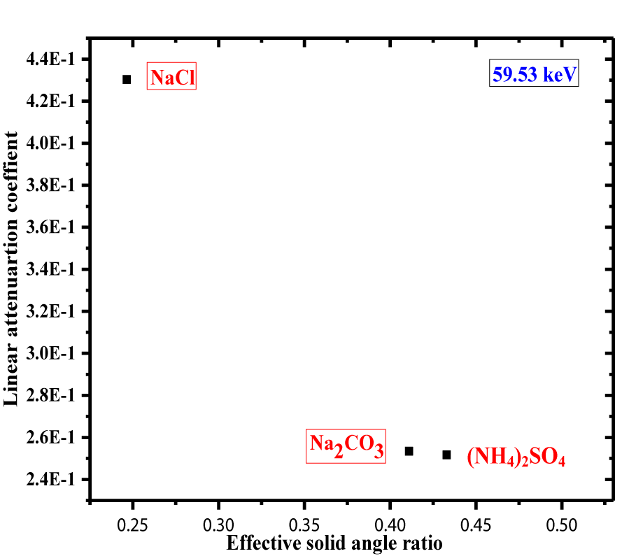
Figure 5: Relation between the linear attenuation coefficient of the samples at 59.54 keV and the effective solid angle ratio.
CONCLUSIONS
In this study, the detectors were used simply without a collimator and applied in a typical laboratory work to determine the linear attenuation coefficient in environmental samples. The experimental method was modeled mathematically by the direct mathematical method and excluding the coherent scattering coefficient of the samples and the detector stuff. This method was verified under the assumption that the density is uniform in the cylindrical sample. The deviation percentages show the possibility of the method was within ̴ 5%. The method could be practical and assist the unskilled technicians in the usual measurements of gamma-ray spectrometry for unfamiliar samples as a cheap and useful method.
REFERENCES
- Knoll GF. Radiation Detection and Measurement. Third edition. (Wiley, 2000)
- Abbas MI, Selim YS, Bassiouni M. HPGe detector photopeak efficiency calculation including self-absorption and coincidence corrections for cylindrical sources using compact analytical expressions. Radiat Phys and Chem. 2001; 61: 429-431. Ref.: https://goo.gl/uNMCQ6
- Hernandez F, El-Daoushy F. Nucl Instrum Methods. Phys Res. A Accel Spectrom Detect Assoc. Equip. 2002; 484: 625-641.
- Robu E, Giovani C. Rom. Rep Phys. 2009; 61: 395-300.
- Berger MJ, Hubbell JH, Seltzer SM, et al. NIST, PML, Radiation and Biomolecular Physics Division. 2010
- Jalali M, Mohammadi A. Gamma ray attenuation coefficient measurement for neutron-absorbent materials. Radiat Phys and Chem. 2008; 77: 523-527. Ref.: https://goo.gl/UsgM1t
- Midgley SM. Measurements of the X-ray linear attenuation coefficient for low atomic number materials at energies 32-66 and Full-size image (<1 K). Radiat Phys and Chem. 2005; 72: 525-535. Ref.: https://goo.gl/RCN6Ow
- Rettschlag M, Berndt R, Mortreau P. Nucl Instrum Methods Phys Res A: Accel Spectrom Detect Assoc Equip. 2007; 581: 765-771. Ref.: https://goo.gl/h6GDal
- Seven S, Karahan IH, Bakkaloglu OF. The measurement of total mass attenuation coefficients of CoCuNi alloys. J Quant Spectrosc Radiat Transf. 2004; 83: 237-242. Ref.: https://goo.gl/CJtmfS
- Badawi MS. Accurate calculation of well-type detector geometrical efficiency using sources with different shapes and geometries. Journal of Instrumentation. 2015; 10. Ref.: https://goo.gl/q0BuFQ
- Abbas MI. Direct mathematical method for calculating full-energy peak efficiency and coincidence corrections of HPGe detectors for extended sources. Nucl Instrum Meth. 2007; 256: 554-557. Ref.: https://goo.gl/jKwFlE
- Abbas MI. A new analytical method to calibrate cylindrical phoswich and LaBr3(Ce) scintillation detectors. Nucl Instrum Meth. 2010; 621: 413-418. Ref.: https://goo.gl/AxlCuG
- Thabet AA, Dlabac AD, Jovanović SI, Badawi Mohamed S, Mihaljevic Nikola N, et al. Nuclear Technology & Radiation Protection. 2015; 30: 35-46. Ref.: https://goo.gl/VSnZSI
- Badawia MS, Abd-Elzaherb M, Abouzeid A Thabetc, Ahmed M. El-khatib. An empirical formula to calculate the full energy peak efficiency of scintillation detectors. Applied Radiation and Isotopes. 2013; 74: 46-49. Ref.: https://goo.gl/k5DOq6
- Badawi MS, Ruskov I, Gouda MM, El-Khatib AM, Alotiby MF, et al. A numerical approach to calculate the full-energy peak efficiency of HPGe well-type detectors using the effective solid angle ratio. Journal of Instrumentation. 2014; 9: Ref.: https://goo.gl/kuuoYF
- El-Khatib AM, Badawi MS, Thabet AA, Jovanovic SI, Gouda MM, et al. Well-type NaI(Tl) detector efficiency using analytical technique and ANGLE 4 software based on radioactive point sources located out the well cavity. Chinese Journal of Physics. 2016; 54: 338-346. Ref.: https://goo.gl/XVXm3R
- Badawi MS. A numerical simulation method for calculation of linear attenuation coefficients of unidentified sample materials in routine gamma ray spectrometry. Nuclear Technology and Radiation Protection. 2015; 30: 249-259. Ref.: https://goo.gl/BKJ6JL