1. Introduction

any irrelevant and redundant genes in gene expression data, which can simplify the learning model by using a strict minimum num Ranked second among 36 kinds of cancers, breast cancer has the ber of predictors, and thus improving breast cancer risk prediction greatest number of incidences and moralities among females worldperformance [4]. In terms of contribution to this research field, this wide. As per a recent publication of the WHO (World Health study proposes a new Decision Tree model-based gene selection Organization), in 2018, 627,000 females were estimated to lose approach, which incorporates two stages: fisher-score-based ranked their lives from this disease, representing approximately 15% of all technique and the gene selection capability of the C5.0 algorithm. cancer deaths among females worldwide. According to the same The ranked method consists in reducing the computational cost by source, early detection is becoming a critical tool to reduce breast removing non-informative genes from the original gene expression cancer morbidity and mortality [1]. At present, breast mammogram data, while the C5.0 algorithm consists in identifying the optimal and ultrasound images are the most traditionally used breast cancer subset of genes, which are quite informative to classify patients. detection techniques. However, besides their high computational

Finally, the genes contained in the obtained gene subset are used cost, these techniques may lead to an overdiagnosis (false positives), as predictors to construct an ensemble of predictive models using 6 which can cause serious clinical consequences, including death from learning algorithms: Random Forests (RF), Support Vector Machine the side effects of a potential Overtreatment [2]. An alternative to

(SVM), Logistic Regression (LR), K-Nearest Neighbors (KNN), Arthis technique is to take the advantages of both data mining and tificial Neural Network (ANN) , and C5.0 Decision Tree algorithm. gene expression technology to predict breast cancer. However, this

In the next section, we briefly outline existing approaches. Methodalternative is not without challenges since the significant number of ology and Materials are described in section 3. Section 4 is devoted non-informative features in gene expression data may increase the to discussing all experiment results. The final section concludes the search space size, which makes gene analysis an impossible task proposed work.

[3]. In the context of this new alternative, a gene selection phase is mandatory to deal with the problem of high-dimensionality in gene

2. Existing literature

From different approaches, a variety of studies have been proposed on breast cancer risk prediction.

Through the implementation of Random Forest(RF) and Extreme Gradient Boosting (XGBoost) , S. Kabiraj et al. predicted breast cancer with an accuracy of 74.73% and 73.63%, respectively[5].

Using the breast cancer Coimbra dataset provided by the University of California Irvine (UCI), Naveen et al., proposed 6 machine learning-based prediction models. The learning process was initialized by a Z-Normalization and cross-validation technique. Experimental results show that the Decision tree and KNN algorithms achieved the highest prediction performance [6]. Agarap proposed a deep learning-based approach on normalized features implementing rectified linear units (ReLU) as the activation function, while the Softmax function as the classifier function. The average cross-validation performance using 10-fold does not exceed 87.96% in terms of accuracy on WBCD (Wisconsin Breast Cancer Data) dataset[7]. S. S. Prakash and K. Visakha also proposed a deep neural network-based approach to predict breast cancer. The authors optimized the neural network model using the early stopping mechanism and dropout layers to avoid overfitting problems. The selected predictors were obtained from the WBCD provided by UCI

[8].

Using gene expression signature, Turgut et al., in their work, first proposed 8 machine learning-based predictive models without using any gene selection algorithms. Then they combined the proposed machine learning algorithms with two feature selection methods: RLR (Randomized Logistic Regression) and RFE (Recursive Feature Elimination). The most striking results concern the SVM algorithm since it achieved the best accuracy of 88.8% after using the selection process [9]. In the same context of gene expression data, Al-Quraishi et al. presented a breast cancer prediction model based on an ensemble classifier using FCBF (Correlation-based filter ) algorithm. Compared to the existing works, their framework achieved an accuracy of 96.11% by involving 112 genes [10]. Aldryan et al. developed a prediction framework using MBP (Modified Backpropagation) with Conjugate Gradient Polak-Ribiere and the standard ACO (Ant Colony Optimization). The MBP was used as a classifier, while the ACO as a gene selection technique. For breast cancer classification using MBP without gene selection, they get the average F-Measure score of 0.2328. After combined with the feature selection using the ACO algorithm, it obtains an average of 0.6412 in terms of performance by involving 2448 genes [11]. Jain et al. presented a two phases-based hybrid feature selection strategy. Their approach combines the Correlation-based Feature Selection (CFS) with the improved-Binary Particle Swarm Optimization (iBPSO) algorithm. The proposed strategy was assessed using Naive–Bayes (NB) algorithm, and the experiments results showed an accuracy of 92.75% for breast cancer classification using an average of 32 genes [12]. To overcome class imbalance issue and time consumption of their old gene selection approach, Li et al. introduced a more efficient implementation of linear support vector machines based recursive feature elimination system (SVM-RFE). Their proposed approach was assessed on 6 public gene expression datasets, and results demonstrated a slight enhancement in terms of time consumption and prediction performance [13].

3. Research methodology

3.1    Description

Using gene expression data, the present paper proposes a new framework that improves breast cancer prediction performance. Figure1 summarizes the main steps of the proposed framework, where fisher score combined with C5.0 are used to select a small number of informative features, and ANN, SVM, KNN, LR, RF , and C5.0 algorithms are applied to the new gene subset to assess the effectiveness of the proposed gene selection approach. The overall pseudo-code of the whole prediction system is illustrated in Algorithm 1 . -discussed in the following sections.

Algorithm 1: Our proposed prediction system

Function Classification(Training set, Test set):

List Classifiers = [SVM, LR,C5.0, ANN, KNN,RF]

/* iterate over all proposed machine learning

algorithms           */ for each Classifiers in List Classifiers do

Model ←Train classifier on the Training set

Test the Model on the Test set

Calculate average performance (Accuracy , F1-score, and the AUC).

Return All obtained Models with their average performances

      /* Main program                                                                       */

       Input     :-A p-diemsional DNA microarray dataset

D = [y, x₁, x₂,…, x_p]_n×1 , with n is the number of samples, x is the gene vector , y is the target vector and p is the number of genes

Output: List of generated prediction models with their average performance and running time for each one.

• Split data D using the stratified K-fold cross-validation technique.;
• for each fold in D do
• D_test ← fold ;
• D_train ← remaining (K − 1)folds ;

               /* Standardization of D_train and D_test using (12)            */

• S Dtrain,S Dtest ← Standardization(Dtrain, Dtest);

              /* Filtering data using Fisher ratio using (1)                 */

• Ftrain, Ftest ← Filter(S Dtrain,S Dtest);

             /* Selection of the optimal gene subset using C5.0     */

• Subtrain,Subtest ← C0(Ftrain, Ftest);

             /* Classification using the optimal gene subset           */

• Models ← Classification(Sub_train,Sub_test);
• Return all generated prediction models ”Models”

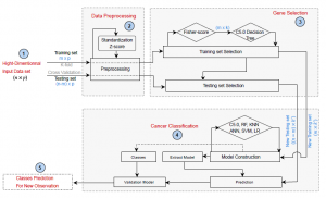
Figure 1: The proposed Framework

3.2    Genes selection strategy

Feature selection is an important stage in intelligent systems modeling, especially in prediction systems [14, 15]. The feature selection or gene selection in the context of microarray data analysis is a useful technique that can reduce dimensionality by removing any redundant, irrelevant, or noisy genes, which can lead to improve the classification performance and reduce the cost of computation [4], [16]–[18]. As shown in Figure 2, gene selection process can be reformulated as follows: given an original set of p genes,

X = (X₁, X₂,.., X_p), find a subset of genes X_sub = (X_i1, X_i2,.., X_ik<<p) such that the most informative genes are selected.

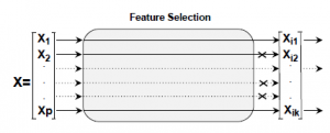
Figure 2: Feature Selection process

Here we present a novel gene selection strategy composed of two steps -Fisher score combined with the C5.0 algorithm- presented into the sequel.

3.2.1     Filter method using Fisher score

Because it acts independently of any classification process, Fisher score-based filter technique is considered as a fast supervised feature selection technique, the reason why it is frequently used when it comes to working with a large number of features (genes) [19]. It can be reformulated as follows: given an input data matrix G of genes, then the Fisher score of each gene (denoted by F) j can be represented by (1) :

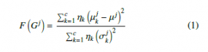
With ^µ_k^j,σ_k^j are the mean and standard deviation of k-th class, corresponding to the j-th feature. µ^j denotes the mean of the whole j-th gene in the G matrix.

As the F of each gene is calculated independently from original genes, only 10% of the highest-ranked genes were selected to achieve the second round of our proposed gene selection strategy.

3.2.2      C5.0 Decision Tree

C5.0 is a new decision tree algorithm developed from C4.5, which has proved its high detection accuracy in many research fields. Compared to C4.5, C5.0 can handle different types of data, deal with missing values, and support boosting to improve classification accuracy [20]. Besides its ability in classification tasks, C5.0 was was used as an efficient feature selection technique in many research Fields [21]–[24]. In the present work, we take both advantages of

C5.0, its ability as a powerful feature selection method combined with the Fisher score-based filter technique, and as a classifier to achieve the classification task in our whole prediction framework.

In the context of gene selection using C5.0 Decision Tree, all genes were initially compared by using the following process: first of all, we set the pruning degree (Pruning is an inherent technique that consists in reducing the size of decision trees by getting rid of branches of the tree that provide little information which can reduce the complexity of the classifier, thus improving classification performance) to 75% as a default value to prevent overfitting. Then, the information gain ratio of each gene is calculated using the formula

(2).

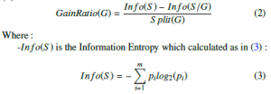
With m the number of classes in the training set (in our case m=2), S a given set of n samples (|S | = n) , and p_i = _|ⁿ_Sⁱ_| the probability that an object in S belongs to the class C_i (with n_i the number of samples that belong to the class C_i )

–Info(S/G) denotes the Conditional Information Entropy which is defined as in (4):

Assuming that G divide the set S into ν subsets (S₁,S₂,…,S _ν), then n_ij denotes the number of classes C_i samples in the subset S _j with

|S j| = Pmi=1 nij and |S | = n. –S plit(G) is defined as in (5) :

The most informative gene (best predictor) with the maximum information gain is selected to be the root node of the whole tree. Then, the root node in each level of the tree is selected from remained genes using the same principle. The gene selection process continues until a maximum depth is meet. As the tree was pruned, the optimal gene subset is determined [20, 25].

4. Classification Algorithms

4.1     Artificial Neural Network

The ANN is a form of distributed computation inspired by networks of human biological neurons. Typically, an ANN consists of a set of interconnected artificial neurons that are organized in several layers called, input, output, and one or several hidden layers. In a typical 3-layer network as shown in Figure fig :ANN, each neuron in a layer is connected to the all next layer neurons with no interconnectivity among the neurons of the same layer and no connection back. All the connections are defined by weight values denoted by w. In the input layer, all nodes get information from the outside and pass it to the nodes of the next layer. Each node computes the weighting sum of all the N neurons of the previous layer and passes it through an activation function (usually logistic) [26]

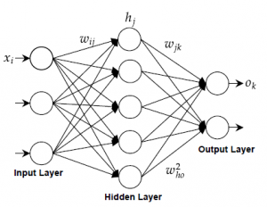
Figure 3: Artificial Neural Network diagram

4.2    Random Forest

As a powerful supervised pattern classification algorithm, RF is used in many intelligent systems. Random Forest is viewed as a combination of several independent decision tree classifiers. Each decision tree is constructed using a randomly selected subset of features. In RF, a majority voting process is used to affect samples to one of the classes by taking the most popular class among all predicted classes by all the tree predictors in the RF [27]. Many processes are used to construct a decision tree classifier; the most commonly used are the Information Gain (IG) and the Gini Index (GI) [28]. In the present paper, we used the GI for the random feature selection measure.

4.3    K-Nearest Neighbors

K-Nearest Neighbors is an easy and simple machine learning algorithm that is widely used in many domains of pattern classification. As the KNN is a non-parametric classifier, new samples are affected to the class represented by a majority of its K-nearest neighbors using a feature similarity rule; since there is no mathematical model to predict labels for new samples. The similarity process is defined using different distance metrics such as Hamming Distance, Euclidean Distance, and Minkowski distance [29] . In the present work, the similarity is measured between K-nearest neighbors using the Euclidean distance metric as in(6), and the number of neighbors K is set to k=4.

Where S₁ and S₂ are two given samples and p is the number of features .

4.4     Logistic Regression

As an extension of the linear regression algorithm for classification problems, Logistic Regression aims to find the best fitting model, which squeezes the output of a linear equation between 0 and 1 using the logistic function. In linear regression, the relationship between output and features is modeled by using a linear equation. However, in a classification problem, it is strongly recommended to have probabilities between 0 and 1, which can force the outcome to be only between 0 and 1 using (7).

4.5    Support Vector Machine

The SVM is a binary classifier algorithm that has been successfully applied in many pattern recognition areas. In linear classification, SVM constructs a classification hyper-plane that separates the data into two sets by maximizing the margins and minimizing the classification error. The hyper-plane is constructed in the middle of the maximum margin. Thus, samples above the hyper-plane are classified positives. Otherwise, they are classified as negatives (Figure 4). SVM is a linear classifier algorithm, meaning that it uses a linear separation to classifier samples. However, in real intelligent systems, datasets are often linearly non-separable. To overcome this problem of non-linearity, a nonlinear transformation of the input vectors into a new feature space is performed, and then a linear separation is performed using the new feature space. In this work, the Gaussian kernel using (8 ), was used to overcome the non-linearity issue.

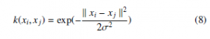
Where: k x_i − x_j k² denotes the Euclidean distance and σ a positive parameter which denotes the smoothness of the kernel.

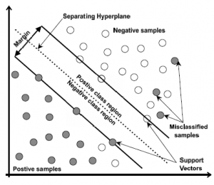
Figure 4: SVM diagram

4.6    Evaluation Metrics

The data mining process has several ways to check the performance of any classification model. The quality of any classification model is built from the confusion matrix (see Figure fig :CM), which summarizes the comparison between predicted and observed classes for all samples. Different types of evaluation measure are calculated from the confusion matrix, and the most commonly used in practice are the classification accuracy as in (9), and F1-score as in (10).

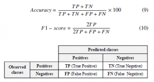
Figure 5: Confusion Matrix for binary classification

Another common evaluation metric used in Machine Learning is the receiver operating characteristic (ROC) curve, which is created by plotting the True Positive Rate (TPR=TP/(TP+FN)) against the False Positive Rate (FPR=FP/(FP+TN)). The Area Under the ROC Curve (AUC) provides a good idea about model performance. The model that gives 100% of corrects predictions has an AUC of 1, while the model that gives 100% of wrong predictions has an AUC of 0.

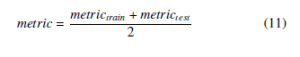
In the present paper, the average of each evaluation metric (described above) in training and test sets is calculated to evaluate the quality of each prediction model using (11).

5. Experimental results and discussion

Before presenting our experimental results in the next section, we describe the gene expression data set used in this paper, K-Fold cross-validation, data preprocessing, and the system configuration.

5.1    Breast cancer dataset details

The proposed prediction framework was conducted on the public available microarray breast cancer dataset [30], which includes 24,481 features with 97 samples, 51 (52.58%) of which are healthy and 46 (47.42%) are diagnosed with breast cancer. Details of our used microarray dataset are given in Table 1.

Dataset	Genes	Samples	Classes	Ref
Breast cancer	24481	97	Relapse/Non-relapse	[30]

Table 1: Microarray datasets details

5.2     Stratified 10-fold Cross-validation

In order to avoid overestimating prediction, a stratified 10-fold cross-validation technique was employed. By using this technique, samples are split into five equal folds (subset) of samples. One of the 10- fold is used for the testing step, and the remaining four folds are put together to form the training data. This process is repeated ten times. The stratification process was used to ensure that all folds are made by preserving the same percentage of samples for each class.

5.3    Preprocessing

Before supplying the datasets to our analysis system (Figure 1), it was necessary to perform a data preprocessing as it is an important step to overcome data imbalance issue. In the present paper, Gene expression levels for each gene were standardized using (12). The result is that expression levels for each feature have a mean 0 and variance 1.

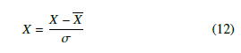
Where: X the overall mean of the feature X and σ its standard

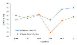
Figure 6: Classification performance with and without our proposed gene selection approach

5.5     Results and discussion

In order to see how good our new approach behaves in situations where there is a large number of genes versus few observations, this section aims at analyzing the results of our proposed framework in terms of classification accuracy, degree of dimensionality reduction, and the running time.

To prove the power of our gene selection approach in terms of prediction performance, we first applied our six proposed machine learning algorithms on the whole breast cancer gene expression data set (without using any feature selection process). Table 2 presents the experimental results and shows the classification performance in terms of accuracy, F1-score, and AUC of each constructed classifier. As we can notice, the most striking performance was achieved by the ANN classifier, which does not exceed 86.99%, while the KNN algorithm shows the lowest performance rate of 64.62%. Almost the classification performances of all constructed classifiers do not exceed the eighties in terms of all evaluation metrics.

Table 2: Performance measurement without gene selection

Classification Model	Time (s)	Accuracy (%)	F1-score	AUC
ANN	42	86.99	0.84	0.85
KNN	1	64.62	0.65	0.65
LR	13	83.91	0.83	0.84
RF	1	83.71	0.86	0.84
SVM	1	80.05	0.79	0.8
C5.0	25	79.01	0.79	0.8

Table 3: Performance measurement using our framework Input Data Original Genes Number Gene Selection approach Selected Genes Classification Model Time (s) Accuracy (%) F1-score AUC Fisher score (F) C5.0 Breast Cancer gene expression data p=24481 k=2448 k’=5 NM 013438, AL137615, NM 003477, Contig26768 RC, Contig55662 RC FC5.0-RF 31 95.00 0.94 0.95 FC5.0-C5.0 31 93.28 0.94 0.97 FC5.0-ANN 31 86.21 0.89 0.86 FC5.0-SVM 31 85.4 0.86 0.85 FC5.0-LR 31 81.78 0.82 0.81 FC5.0-KNN 31 80.4 0.82 0.8 -50   FC5.0-C5.0     FC5.0-RF Training = 41 46 Training = 0 0 Test = 5 Test = 0 Training = 0 1 Training = 46 50 Test = 1 Test = 4 0 1 0                                              1   FC5.0-SVM   Training = 40 45 Training = 1 1 0 1 Training = 37 41 Training = 4 5 Test = 5 Test = 0 Test = 4 Test = 1 Training = 2 3 Training = 44 48 Training = 4 5 Training = 42 46 Test = 1 Test = 4 Test = 1 Test = 4 0 1   0 1     FC5.0-KNN     FC5.0-LR Training = 28 33 Training = 13 13 Test = 5 Test = 0 Training = 10 11 Training = 36 40 Test = 1 Test = 4 0 1 0                                              1   FC5.0-ANN   Training = 36 39 Training = 5 7 0 1 Training = 26 31 Training = 15 15 Test = 3 Test = 2 Test = 5 Test = 0 Training = 3 4 Training = 43 47 Training = 9 9 Training = 37 42 Test = 1 Test = 4 Test = 0 Test = 5 0 1   0 1

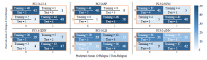
Figure 8: Confusion Matrix of our shrinkage models

Table 3 shows the experimental results of our gene selection method when used along with our proposed machine learning algorithms. The results are presented in terms of classification performance matched with the number of selected genes. As we can notice, using our approach, the dimensionality of our research space (the number of genes) was reduced in two phases. First, the number of genes passed from p=24481 (the original number of the gene as shown in Table 1) to k=2448 using the Fisher ratio-based filter method, the new k represents 10% of the original number of genes that have the highest score. In the second phase, the number of previously selected genes k was reduced for a second time using the inner feature selection ability of C5.0 Decision Tree algorithm; thus, the k passed from 2448 genes to five genes (k’=5). Thereafter, the new subspace of k’=5 predictors (genes) was used to construct the ensemble of classifiers (SVM, KNN, LR, ANN, C5.0, and RF). As we can see from experiment results (Table 3 and Figure 6), almost all constructed shrinkage models produced a classification performance that could exceed the eighties; and the most striking result concerns the FC5.0-RF and FC5.0-C5.0 models since they achieved the best prediction performance that could reach respectively to 95% and 93.28% in terms of all evaluation metrics, which is much better than what was reported in the first experiment (without applying gene selection Table 2). In contrast, the prediction performance has slightly deteriorated when it comes to LR and ANN classifiers when using our gene selection approach.

In Figure 7, the ROC curves are plotted to estimate the AUC of each constructed classifier model when using our gene selection method, which can help to compare their prediction performances. As we can see from this figure, ROC curves of FC5.0-RF and FC5.0C5.0 models are the closest to the perfect performance curve, which can explain the quality of these models reported in Table 3. In the same context of the second experiment using our gene selection approach, Figure 8 gives a better overview of the relations between our generated prediction models outputs and the true labels. As we can notice, for our favorite model (FC5.0-RF) all samples in the training set are correctly classified, while in the test set, only one sample out of 10 is miss-classified, which confirms the achieved average classification accuracy of 95%.

According to all results reported above, it can be summed up that the power of our whole system (illustrated in Figure1)) comes from its ability to predict breast cancer risk with high performance by involving a bar minimum of genes predictors (only five genes).

Table 4 compares the performance (in terms of accuracy and the number of selected genes) of our gene selection-based breast cancer classification technique with existing gene selection methods. The comparison is made to demonstrate the capability of our approach over other techniques in predicting breast cancer. As it can be noticed, the proposed approach led to a higher prediction performance by involving only five genes, which is much better than was reported for the other techniques.

Table 4: Comparison of the proposed FC5.0 approach with other feature selectionbased approaches

Paper

Appraoch

# Selected genes

Best accuracy (%)

RFE+SVM           88,82 [9]  50

	RLR+SVM		87,87
[10]	FCBF+DNN+SVM	112	96.11
[11]	ACO+MBP	2448 (10%)	64.12
[12]	CFS+iBPSO+NB	32	94.00
[13]	SVM-VSSRFE	–	90.03
Ours	FC5.0-RF	5	95.00

6. Conclusion

By using gene expression data to improve breast cancer risk prediction, this study proposed a new Decision Tree model-based gene selection strategy, which incorporates two stages: fisher score-based filter method and the feature selection capability of the C5.0 algorithm. The prefiltering phase using the Fisher score aims at reducing the dimensionality of breast cancer gene expression data by getting rid of any irrelevant or redundant genes in the predictive genes. Then in the second stage, we make use of the obtained low-dimensional research space to find the best gene subset that maximizes the prediction performance by using the feature selection capability of the C5.0 decision tree algorithm. The optimal genes subset was used as the input for cancer classification using six machine learning algorithms. To prove the impact of our approach on breast cancer risk prediction, we compared the classification performance of our generates models between them and with the performance of classifiers without using any gene selection process. Experimental results show that our gene selection approach led to a higher prediction performance that reached 95% using FC5.0-RF model by taking fewer genes, which is better than what was reported in Table 2 and Table 4 .

This work can be enhanced in two different aspects: the classification models and the search engine. For the classification model, we intend to propose the use of other supervised machine learning algorithms in order to achieve more accurate results in terms of prediction. For the search engine, other gene selection approaches can be proposed or combined with our proposed one. We expect these improvements to predict breast cancer risk with high accuracy, which may guide further breast cancer researches.

1. “WHO | Breast cancer,” Publisher: World Health Organization.
2. “Determining relevant biomarkers for prediction of breast cancer using anthro- pometric and clinical features: A comparative investigation in machine learning paradigm,” Biocybernetics and Biomedical Engineering, 39(2), 393–409, 2019, doi:10.1016/j.bbe.2019.03.001, number: 2 Publisher: Elsevier.
3. J. Cao, L. Zhang, B. Wang, F. Li, J. Yang, “A fast gene selection method for multi-cancer classification using multiple support vector data description,” Journal of Biomedical Informatics, 53, 381–389, 2015, doi:10.1016/j.jbi.2014. 12.009.
4. H. Moutachaouik, I. El Moudden, “Mining Prostate Cancer Behavior Using Parsimonious Factors and Shrinkage Methods,” SSRN Electronic Journal, 2018, doi:10.2139/ssrn.3180967.
5. S. Kabiraj, M. Raihan, N. Alvi, M. Afrin, L. Akter, S. A. Sohagi, E. Podder, “Breast Cancer Risk Prediction using XGBoost and Random Forest Algorithm,” in 2020 11th International Conference on Computing, Communication and Networking Technologies (ICCCNT), 1–4, 2020, doi:10.1109/ICCCNT49239. 2020.9225451.
6. R. K. Sharma, A. Ramachandran Nair, “Efficient Breast Cancer Predic- tion Using Ensemble Machine Learning Models,” in 2019 4th International Con- ference on Recent Trends on Electronics, Information, Communication Tech- nology (RTEICT), 100–104, 2019, doi:10.1109/RTEICT46194.2019.9016968.
7. A. F. Agarap, “Deep Learning using Rectified Linear Units (ReLU),” CoRR,
   abs/1803.08375, 2018.
8. S. S. Prakash, K. Visakha, “Breast Cancer Malignancy Prediction Using Deep Learning Neural Networks,” in 2020 Second International Conference on Inventive Research in Computing Applications (ICIRCA), 88–92, 2020, doi: 10.1109/ICIRCA48905.2020.9183378.
9. S. Turgut, M. Dagtekin, T. Ensari, “Microarray breast cancer data classifi- cation using machine learning methods,” in 2018 Electric Electronics, Com- puter Science, Biomedical Engineerings’ Meeting (EBBT), 1–3, 2018, doi: 10.1109/EBBT.2018.8391468.
10. T. Al-Quraishi, J. H. Abawajy, N. Al-Quraishi, A. Abdalrada, L. Al-Omairi, “Predicting Breast Cancer Risk Using Subset of Genes,” in 2019 6th Interna- tional Conference on Control, Decision and Information Technologies (CoDIT), 1379–1384, IEEE, Paris, France, 2019, doi:10.1109/CoDIT.2019.8820378.
11. D. P. Aldryan, Adiwijaya, A. Annisa, “Cancer Detection Based on Microarray Data Classification with Ant Colony Optimization and Modified Backpropaga- tion Conjugate Gradient Polak-Ribie´re,” in 2018 International Conference on Computer, Control, Informatics and its Applications (IC3INA), 13–16, IEEE, Tangerang, Indonesia, 2018, doi:10.1109/IC3INA.2018.8629506.
12. I. Jain, V. K. Jain, R. Jain, “Correlation feature selection based improved-Binary Particle Swarm Optimization for gene selection and cancer classification,” Ap- plied Soft Computing, 62, 203–215, 2018, doi:10.1016/j.asoc.2017.09.038.
13. Z. Li, W. Xie, T. Liu, “Efficient feature selection and classification for mi- croarray data,” PLOS ONE, 13(8), e0202167, 2018, doi:10.1371/journal.pone. 0202167, number: 8.
14. I. El Moudden, H. Jouhari, M. Ouzir, S. bernoussi, “Learned Model For Human Activity Recognition Based On Dimensionality Reduction,” 2018.
15. I. El Moudden, S. Lhazmir, A. Kobbane, “Feature Extraction based on Principal Component Analysis for Text Categorization,” 2017, doi:10.23919/PEMWN. 2017.8308030.
16. I. El Moudden, M. Ouzir, S. ElBernoussi, “Feature selection and extraction for class prediction in dysphonia measures analysis: A case study on Parkinson’s disease speech rehabilitation,” Technology and health care: official journal of the European Society for Engineering and Medicine, 25, 1–16, 2017, doi: 10.3233/THC-170824.
17. M. Hamim, I. E. Moudden, H. Moutachaouik, M. Hain, “Decision Tree Model Based Gene Selection and Classification for Breast Cancer Risk Prediction,” in Smart Applications and Data Analysis, 165–177, Springer, Cham, 2020, doi:10.1007/978-3-030-45183-7 12.
18. M. Hamim, I. El Mouden, M. Ouzir, H. Moutachaouik, M. Hain, “A NOVEL DIMENSIONALITY REDUCTION APPROACH TO IMPROVE MICROAR- RAY DATA CLASSIFICATION,” IIUM Engineering Journal, 22(1), 1–22, 2021, doi:10.31436/iiumej.v22i1.1447.
19. Q. Gu, Z. Li, J. Han, “Generalized Fisher Score for Feature Selection,” arXiv:1202.3725 [cs, stat], 2012.
20. R. Rathinasamy, L. Raj, “Comparative Analysis of C4.5 and C5.0 Algorithms on Crop Pest Data,” International Journal of Innovative Research in Computer and Communication Engineering, 5, 2017, 2019.
21. Y. Y. Wang, J. Li, “Feature-Selection Ability of the Decision-Tree Algorithm and the Impact of Feature-Selection/Extraction on Decision-Tree Results Based on Hyperspectral Data,” Int. J. Remote Sens., 29(10), 2993–3010, 2008, doi: 10.1080/01431160701442070.
22. D. McIver, M. Friedl, “Using Prior Probabilities in Decision-Tree Classifica- tion of Remotely Sensed Data,” Remote Sensing of Environment, 81, 253–261, 2002.
23. Z. Qi, A. G.-O. Yeh, X. Li, Z. Lin, “A novel algorithm for land use and land cover classification using RADARSAT-2 polarimetric SAR data,” Remote Sensing of Environment, 118, 21 – 39, 2012, doi:https://doi.org/10.1016/j.rse. 2011.11.001.
24. L. Deng, Y.-n. Yan, C. Wang, “Improved POLSAR Image Classification by the Use of Multi-Feature Combination,” Remote Sensing, 7, 4157–4177, 2015.
25. S.l. PANG, J.-z. GONG, “C5.0 Classification Algorithm and Application on In- dividual Credit Evaluation of Banks,” Systems Engineering – Theory & Practice, 29(12), 94 – 104, 2009, doi:https://doi.org/10.1016/S1874-8651(10)60092-0.
26. S. Rajasekaran, G. A. V. Pai, Neural networks, fuzzy logic, and genetic algo- rithms : synthesis and applications, New Delhi : Prentice-Hall of India, eastern economy ed edition, 2003, includes bibliographical references and index.
27. A. Chowdhury, T. Chatterjee, S. Banerjee, “A Random Forest classifier-based approach in the detection of abnormalities in the retina,” Medical & Biological Engineering & Computing, 57, 2018, doi:10.1007/s11517-018-1878-0.
28. M. Pal, “Random forest classifier for remote sensing classification,” Interna- tional Journal of Remote Sensing – INT J REMOTE SENS, 26, 217–222, 2005, doi:10.1080/01431160412331269698.
29. R. O. Duda, P. E. Hart, D. G. Stork, Pattern classification, Wiley, New York, 2nd edition, 2001.
30. L. J. van ’t Veer, H. Dai, M. J. van de Vijver, Y. D. He, A. A. M. Hart, M. Mao, H. L. Peterse, K. van der Kooy, M. J. Marton, A. T. Witteveen, G. J. Schreiber, R. M. Kerkhoven, C. Roberts, P. S. Linsley, R. Bernards, S. H. Friend, “Gene expression profiling predicts clinical outcome of breast cancer,” Nature, 415(6871), 530–536, 2002, doi:10.1038/415530a, number: 6871.

(Click Here)