
Two Degree-of-Freedom Vibration Control of a 3D, 2 Link Flexible Manipulator
Volume 3, Issue 6, Page No 412-424, 2018
Author’s Name: Waweru Njeria), Minoru Sasaki, Kojiro Matsushita
View Affiliations
Mechanical Engineering, Mechanical Engineering, 1-1 Yanagido, Gifu, Japan
a)Author to whom correspondence should be addressed. E-mail: v3812104@edu.gifu-u.ac.jp
Adv. Sci. Technol. Eng. Syst. J. 3(6), 412-424 (2018); ![]() DOI: 10.25046/aj030649
DOI: 10.25046/aj030649
Keywords: Inverse control, Strain feedback, System stability, Two-degree-of freedom

Export Citations
Considering link vibrations, the main limitation affecting flexible manipulators, this article seeks to make a contribution by presenting an enhanced two degree of freedom vibration controller. This controller uses a filtered right inverse controller in the feedforward and strain feedback controller in the feedback path. The Filtered inverse controller damps transient vibrations while preserving joint trajectories. On the other hand, strain feedback controller ensures a rapid decay of residue vibrations. Modeling of the manipulator was carried out in Maplesim, linearized and inverted in Matlab. Experiments were conducted in the SPACE environment. Both the simulations and the experimental results showed that the two-degree-of-freedom controller yielded a superior performance over the two controllers individually.
Received: 24 October 2018, Accepted: 02 December 2018, Published Online: 15 December 2018
1. Introduction
This journal article, an extension of our original work presented in the 2018 IEEE International conference on Applied System invention(ICASI) [1] seek to make a contribution by presenting a two degree of freedom controller comprising of a filtered inverse controller in the forward path and a Direct Strain Feedback controller(DSFB) in the feedback path. The strength of the proposed methods lies in the fact that it can suppress both the motion induced vibrations, as well as residue vibrations, and it is superior than the individual controllers separately.
Since the dawn of the industrial revolution, over and above making the work easier, man has been thinking of how to replace human labour altogether. This has brought to fruition many kinds of robots and manipulators to fulfil this dream. These robots came handy in carrying out repetitive chores, in hazardous work environment and in heavy industries to mention just but a few. Initially, robots comprised of bulky links driven by huge motors. Thus, they suffered from link inertia or were rather driven at low speeds and were expensive to operate considering the amount of power they consumed and the cost of maintenance. Challenges of rigid robots, except for heavy tasks and for application where low speeds is not a problem, were addressed by the introduction of flexible manipulators.
These Flexible manipulators come with lots of merits over rigid manipulators; like being light in weight hence, small actuators can be used. Also, the maintenance and running costs are low. However, their links are flexible, hence they tend to vibrate especially when operated at high speeds. These vibrations increases with both loading and additional links, due to coupling, which adversely affects the accuracy and duplicity of tasks. Also, link vibration leads to time wastage, hence having to wait for the residue vibrations to decay to healthy levels before the end-effector can be put to use. Link vibrations also raises a safety issue, as continued vibration can lead to mechanical failure due to fatigue, thereby reducing the life span of the manipulator, and posing a risk to the operators.
In a bid to reap all the benefits of the flexible manipulators, a lot research has been done to mitigate link vibrations and all its shortcoming. Researchers [2, 3] introduced a vibration control method for the flexible manipulators based on internal resonance. In their scheme, they designed an absorber comprising of a servomotor, sliding along the links of the manipulator and driving a branched link. At internal resonance, the energy stored in the links in form of vibration energy, is propagated back and forth between the different modes and is dissipated to the absorber. One challenge associated with their method includes the complication in establishing the internal resonance considering the different loading and trajectories. Another limitation is the feasibility of using this scheme with additional links, and the inertia introduced by the absorber.
In [4], the author proposed a novel filtered input shaping technique, implemented inside the position control loop of a single link flexible manipulator. The controller was developed based on the dominant vibration modes of the manipulator to mitigate the motion-induced vibrations from the high speed operations, which arose also from the flexible nature of the link. The controller was based on a lowpass and a bandpass elliptic filters to attenuate dominant modes in the input signal, and avoid exciting the manipulator at its natural frequencies. With fixed filters, however, the performance of their system would deteriorate with additional loading, since dominant modes are bound to change. The limit actions of the fixed filters are addressed in [5]. There exist similar work involving input shaping for vibration control, for example [6–8].
In [9,10], the authors noted that vibrations occur after the manipulator was brought to a sudden stop. They found that the severity of the induced vibration was largely dependent on the initial speed, speed prior to the stop and the duration of the motion. The higher the speed, the longer the vibrations will ensue, before the end pointer settles to the desired position. In their work, they developed trapezoidal and triangular velocity profiles to reduce joint velocities at the beginning of the operation and prior to stopping. In other words, the trajectory was portioned into acceleration period, constant speed period and deceleration period. The scheme resulted in minimal vibrations naturally as the manipulator decelerated to a stop.
Another popular active vibration control technique is the use of smart structures in form of piezoelectric actuators which are bonded to the root of the manipulator [11]. Authors in [12] made use of shunted piezoelectric transducers to mitigate vibrations. In this type of solution, the piezoelectric transducers are bonded onto the links of the manipulator. Link flexure is converted to corresponding voltages which are used as feedback. Under this broad scheme, alternative vibration suppression methods include: Position positive feedback [13], strain rate feedback control [14], quantitative feedback theory [15], and resonant control [16]. Current trends include using Neural Networks to tune PID gains [17], filtered inverse control [18], robust control, in particular H∞ together with piezoelectric actuators [19], boundary control [20].
The rest of the article is organized as follows; Modelling of the two link 3D flexible manipulator is introduced in section 2. Development of the inverse model is highlighted in section 3. Application of the developed inverse is applied to the manipulator 4. Simulation and experimental results are presented and discussed in section 6 followed by conclusion in section 7.
2. Modeling and validation of the manipulator
The basic prerequisite for model based controller designs an accurate model of the plant to be controlled. This is an easy feat for simple systems which can easily be obtained from first principles by paper and pen observing the governing equations. However, for complex system especially if they are nonlinear and dynamic is not an easy task.
Advancements in the processing power of modern computers has brought forth another method of obtaining models of complex system by employing symbolic softwares. Examples of such softwares include but not limited to Maple/Maplesim©, Mathematica©, Matlab/Simscape© all based on Modelica© library. Insymbolicmodeling,mathematical models of common engineering parts such as joints, links, motors with possibilities of customization are dragged onto a workspace to form a complex system. Simulations are carried out considering a practical environment. The strength of this technique lies in its accuracy, simplicity and the possibility of including aspects which cannot be represented mathematically.
The plant reported in this article is a two link, 3D flexible manipulator, with technical description as tabulated in Appendix A.1. It has three rigid joints, driven by dc servomotors and fitted with harmonic drives to reduce joint velocities by a factor of one hundred. It has two flexible links with a variable load attached at the far end of the link number 2.
The control system includes a computer running the Matlab/Simulink and interfaced with dSPACE DSP board, which serves as Servomotors driver via DA converters and collection of data via AD converters. Operation of the system is carried out from the dSPACE control desk environment. The measurement of the joint angles and the velocities were achieved using encoders fitted at the bottom part of the servomotors. Strain data was obtained from strain gauges attached at the root of the links. Strain information was conditioned using wheatstone bridge, filtered and amplified before being transmitted to the computer via AD converters. The control system is configured as in Figure 1.
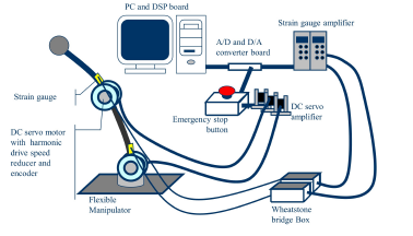 Figure 1: Control system setup
The manipulator and the control system were modelled and linearized in Maple/Maplesim and its inverse model was developed in Matlab. Validation of the model against the actual manipulator was performed and a perfect agreement was observed between the nonlinear model, linearized model and the actual manipulator, as will be seen later in the results. State space matrices of the linearized model are posted in the Appendix A.3.
3. Development of the inverse system
To develop an inverse model, consider an Linear
Time Invariant(LTI) continuous time square system P
(t), and let the triplet A,B and C be a minimal state-space representation. It is assumed that the system is stable or stabilized by negative feedback.
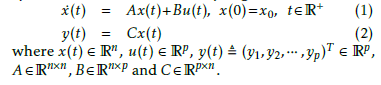 Definition 1. Given P(t), an LTI system defined above in equations 1 and 2, inversion involves the development of a model P−1(t) that yields the input control law uf (t) to reproduces y(t) when used as the input to P(t).
Definition 2. If Ci denotes the ith row of the output matrix C, then the system is said to have a relative degree r , (r1, r2 ··· , rp)T if CiAlB = 0, ∀l < ri − 1; 1 ≤ i ≤ p [21]. Further, if this holds true in the entire domain in the states, then we say the system has a well defined relative degree.
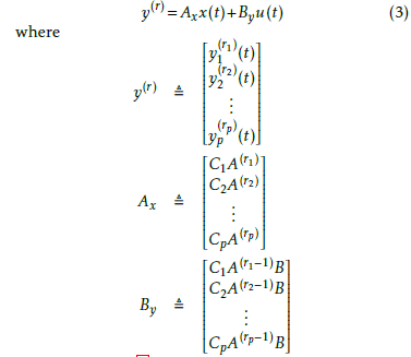
Following Definition 2 above and assuming that the system has a well-defined relative degree r = (r1,r2,··· ,rp)T , differentiating the ith output ri times w.r.t time yields y(ri)=CiA(ri)x+CiA(ri−1)Bu
whereCi is the ith roof the out put matrix C for1≤i≤p and the subscripts represent the Lagrange’s notation of the rith derivative in time. Repeating this for all the rows and having the resulting expressions in vector form, we have
 From equation (3), and the fact that By is invertible because of the well defined relative degree assumption, the control law is
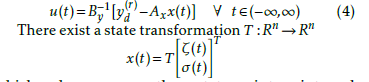
x(t)=T σ(t) which decomposes the states into internal dynamics(system states, which are not directly controlled by the input u(t)), σ(t) and the external dynamics ζ(t), (i.e, the output and its derivatives in time up to (ri−1)) as
![]() The expression of the new system after coordinate
The expression of the new system after coordinate
transformation is ζ˙ = Aˆ1ζ+Aˆ2σ+Bˆ1u σ˙ = Aˆ3ζ+Aˆ4σ+Bˆ2u
where Aˆ =”Aˆˆ1 AAˆˆ24#=T −1AT and Bˆ =”BBˆˆ21#. Replacing
A3 x(t) in (4) with the transformed dynamics, the control law to maintain the exact tracking can be written as
 internal dynamics can now be expressed as
 in the same respect, equation (4) can now be written as
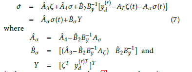
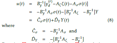 Equation(7)together with equation(8)form the inverse system and can be represented in state space form
![]() and represented as in Figure 2(see Appendix A.4 for details of matrices Aσ,Bσ,Cσ,DY ).
and represented as in Figure 2(see Appendix A.4 for details of matrices Aσ,Bσ,Cσ,DY ).
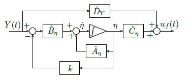 Figure 2: Block diagram of the inverse system
4. Inverting the manipulator
The linear model has 17 states distributed as:
|
• x1(t)=i1(t) • x2(t)=w11(t) • x3(t)=w˙11(t) • x4(t)=w12(t) • x5(t)=w˙12(t) • x6(t)=w21(t) |
• x7(t)=w˙21(t) • x8(t)=w22(t) • x9(t)=w˙22(t) • x10(t)=θ1(t) • x11(t)=θ˙1(t) • x12(t)=θ2(t) |
• x • x • x • x |
13(t)=θ˙2(t) 14(t)=θ3(t) 15(t)=θ˙3(t) 16(t)=i3(t) |
| • x17(t)=i2(t) | |||
whereij denotesthearmaturecurrenttotheservomotor drivingjointj(j =1,2,3), θj andθ˙j aretheinstantaneous joint angles and joint velocities of joint (j = 1,2,3), respectively, whereas (w11,w12), (w21,w22) and their derivatives denote the flexure variable for links 1 and 2 respectively.
Remark 1. In the modelling of the manipulator in Maplesim, the lengths of links 1 and 2 are broken into two to accommodate an instrument to measure the strain. In regard to this, in the linearized model, the flexure variable has two parts as w11,w12 for link 1 and w21,w22 forlink2. Except for having twice as many flexure variables as the number of links, breaking the links does not affect the performance of the model.
With a relative degree of r = (3,3,3), the internal dynamics, σ(t), were taken as the flexure variables, whereas the output variables and their derivatives ζ, were taken as the three joint angles, velocities and motor currents, i.e.
Poles and zeros of the linear model and its inverse are as shown below
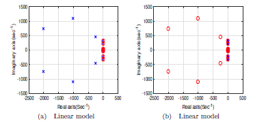 Figure 3: Poles and zeros of the plant and its inverse
Upon inversion, the eight poles corresponded to the internal dynamics, i.e. the flexure variables. These poles were found to be lying on the imaginary axis implying that these variables are marginally stable and that they will not decay to zero with time. This was addressed by applying pole placement technique to slightly shift these poles to the right. This is important as it means that the stability of the internal dynamics and the resulting inverse is assured. Also the stable model still remains to be the inverse of the linear model. Consequently the stable solution of the internal dynamicsfollowsfromsolvingtheODEinequation9as
![]() where τ is a dummy variable. The first term represent the zero-input response whereas the second term is the zero-state response. With negative eigenvalues of the matrix Aσ, which is enforced using pole placement technique, it can be deduced from this expression that the internal dynamics σ(t) are bounded for bounded external dynamics Y(t).
where τ is a dummy variable. The first term represent the zero-input response whereas the second term is the zero-state response. With negative eigenvalues of the matrix Aσ, which is enforced using pole placement technique, it can be deduced from this expression that the internal dynamics σ(t) are bounded for bounded external dynamics Y(t).
Driving the manipulator via an inverse controller implies that the joint angles will follow the desired trajectories exactly. For the high speed operations involving step or square wave trajectories; however, joint velocities during the rising and the falling edges would be too high thus not safe for the operators. It can also lead to mechanical failures. This was addressed by introducing second order bilinear low pass filter, before the inverse controller, of the form f (s)=
where λ is an adjustable parameter for limiting the manipulator speeds to safe levels.
Remark 2. Operation without filter leads to very high speeds, hence exposing the operator and environment to risk, also risking the mechanical well being of the manipulator.
Remark 3. Operation with filters without the inverse controller means that the high frequency components of the trajectories are removed leading to a very high joint error.
Remark 4. The inverse controller ensures that the joint trajectories follows the desired trajectory, the filter ensure safe operation speeds.
5. Direct strain feedback control
The theory of Direct Strain Feedback (DSFB) was developed by Luo [22, 23] and experimented with a one-link flexible manipulator. In this control scheme, the strain measured at the root of the flexible link is multiplied by a constant gain k and the resultant signal is used to modify the control law as a negative feedback. The overall effect of direct strain feedback is to increase the system damping coefficient thereby leading to a rapid decay of transverse vibrations and torsional vibration as a result of coupling between the two types of vibrations. In [22], the author shows that the technique can satisfactorily dampen link vibrations. He also analytically derived the proof that the resulting closed loop is asymptotically stable. A block diagram showing the hybrid of the filtered inverse feedforward controller and the DSFB is shown in Figure 4.
From the figure, the new control law is expressed as u(t)=θf (t)−θ(t)−kε(0,t)
where:
| θf (t) | – | Trajectory tracking signal generated by the filtered inverse controller |
| θ(t) | – | Joint angle of the flexible manipulator |
| ε(0,t) | – | Strain at the root of the links |
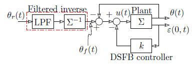 Figure 4: Hybrid control setup
6. Results and Discussion
6.1. Modelling and validation results
To validate the model developed and linearized in section 2, simulations were conducted in Matlab Simulink on the linearized models and the performance of the model compared with the existing flexible manipulator. The task involved moving the joints as in a simple pick and place task popular in industries e.g soldering, painting etc.
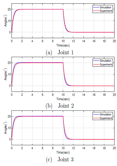 Figure 5: Comparison of Joint angles between linear and the actual manipulator
Figure 5 shows the joint trajectories for joint 1, 2 and 3 for the model and the manipulator. From the figures, we can see a perfect agreement of the model with the existing manipulator.
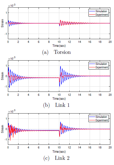 Figure 6: Comparison of strain between linear and the actual manipulator
Figure 6 validates the model employed in this work in terms of the vibrations excited. It shows the strain information of the linear model against the actual manipulator. Perfect agreement between joint angles in torsional and links strain in 6(a-c) can be observed. Observations in figures 5 and 6 leads to the deduction that the linear model represents an accurate model of the manipulator. In addition, the inverse derived from the linearized model represent an accurate inverse of the actual manipulator.
6.2. Simulation results
This section presents simulation results of the validated model subjected to the inverse controller, the strain feedback controller and a hybrid controller of the two. Simulations were conducted in Matlab/Simulink for a desired joint trajectory that involved moving the joints at an angle of 20 degrees for 10 seconds and back to the vertical position for 10 more seconds. Typical application s of such trajectories are in soldering and other pick and place related tasks. Simulink model of the simulation setup is as shown in Figure 7.
The servomotors used here were of the speed reference type. Thus, the angle feedback formed the outer feedback loop, having unity feedback gain, while strain feedback was in the inner loop with a feedback gain k = 0.4. To avoid errors due to self-weight, the gravitational effect is compensated for in the strain signal. The compensation was done by removing the self-weight offset before being fed back through the DSFB controller.
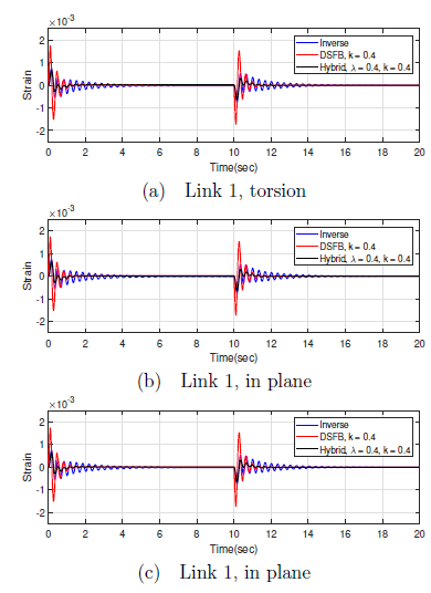 Figure 8: Strain information of the linear model
From the figures of torsional strain(Figure 8a), in plane strain for link 1(Figure 8b) and link 2(8c), it can be seen that the inverse controller had an upper hand in suppressing transient vibrations caused by the sudden starting and sudden stopping. However, these vibrations lasted for a relatively longer time. Interestingly, DSFB, though it had very poor transient response, it was very strong in dealing with residue vibrations. The hybrid of the two controller was inherently better in handling both the transient and the residue vibrations, hence, outperformed the individual controllers.
 Figure 9 gives a pictorial evidence of the of the comparison and the strengths of the individual controllers.
6.3. Experimental results
The experiment involved moving the three joints at an angle of 20 degrees, using a step signal lasting for 10 seconds, followed by returning to its original vertical position for another 10 seconds for a case without tip mass and with a tip mass of 100g. Strain measurement was achieved by attaching strain gauges at the root of respective links for torsional, link 1 in plane and link 2 in plane strain. Figure 10 shows the experimental setup of this work.
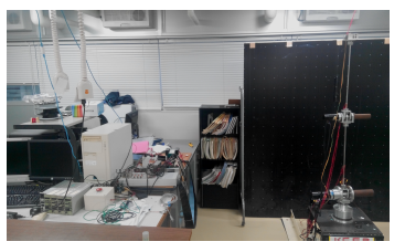 Figure 10: Experiment setup
Figure 11 shows the experimental results for the torsional strain, 11a, and strain for the two links, (11b, 11c) for a manipulator without any tip load. The figures show the comparison of the inverse controller, the DSFB controller and a hybrid of the two. It can be seen that the inverse controller had an upper hand in dealing with motion induced vibrations. On the other hand, the DSFB ensured a rapid decay of the residue vibrations. A combination of the two controllers as a two degree of freedom controller, yielded a system characterised by minimal motion-induced vibrations decaying very rapidly. The hybrid of the two yielded minimal strain amplitudes and shortened the duration of the vibrations. Actually, the overall performance of the hybrid was better than that of the controllers in their areas of strengths, individually. This is attributed to the combined strengths of the two controllers.
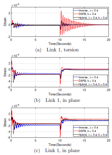 Figure 11: Torsional and lateral strain without any load
In plane strain in the first 10 seconds of the links 1 and 2(11b, 11c), an offset from zero strain can be seen. This error is associated with the fact that, during this time, links 1 and 2 are tilted and thus affected by gravity. Consequently, the bending strain at the root of the links did not converge to zero but remained to be a value of the distortion due to the self weight of the links for the entire period. However, this effect doesn’t affect torsional strain.
Figure 12 shows the strain spectral power density without any load, where the improvement was very significant. It can be seen that individual controllers suppress different frequencies while the hybrid inherits these capabilities, better yet outperforming the individual controllers. Again, the effect of self weight due to the tilted status of links 1 and 2 can be seen in the lower part of the spectrum (Figures 12b,12c), but it is absent in the spectrum for torsional strain (12a).
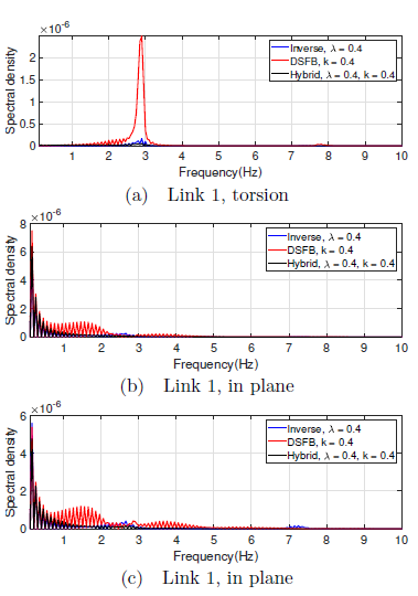 Figure 12: Strain spectral density without any load
With a load of 100g attached at the distal end of link 2, Figure 13 shows the torsional strain(13a) and in plane lateral strain for links 1 and 2(13b,13c). From the figure, the vibrations are a bit severe relative to those experience in a system without load. This is attributed to the fact that loading a flexible manipulator leads to excitation of more severe vibration at a relatively lower frequency when compared to a manipulator without any load. The offset due to self weight imposed by gravity during the first 10 seconds is also relatively higher.
The performance of the inverse controller is commendable in attenuating link vibration, however, complete mitigation is not possible and severe residues remains for the entire duration of operation. Strain feedback on the other hand, though its performance in eradicating the residues is very good, it is poor in dealing with trajectory induced vibrations. The hybrid of the two controllers, having inherited the complementary strengths of each controller is able to deal with both transient and residue vibrations.
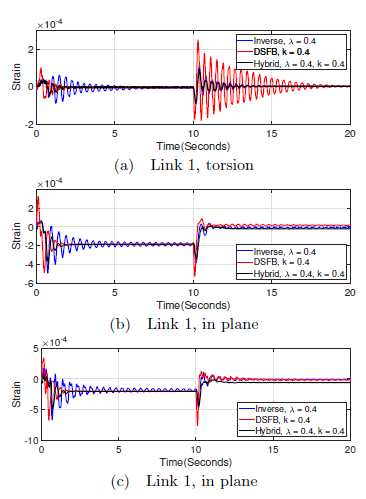 Figure 13: Torsional and lateral strain with a load of 100g
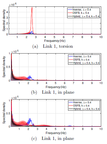 Figure 14: Strain spectral density with a load of 100g
To investigate the effect of loading on the strain spectral power density, Figure 14 illustrates the spectrum for torsional strain(14a) and in plane lateral strain(14b, 14c) for links 1 and 2 respectively. Comparing these frequency responses, wecanobservethat: 1). The peaks are higher than those seen in a system without any load, and 2). these peaks occurred at a slightly lower frequencies.
7. Conclusion
We successfully developed, linearized and validated a model of a 3D, two link, flexible manipulator. A stable right inverse of the linear model was developed, augmented with a low pass filter, and used as a feedforward controller. Together with a direct strain feedback controller, k = 0.4, in the feedback loop, the combination formed a two degree of freedom controller. From both simulations and experimental results, we found the inverse controller has an upper hand in handling motion induced vibrations which arose from sudden starting and stopping. Also, the strain feedback controller ensures rapid decay of the residue vibrations. Finally, the hybrid of the two controllers inherently has the strengths of the two controllers, exhibited a superior performance of suppressing both the transient and the residue vibrations.
- Waweru Njeri, Minoru Sasaki, and Kojiro Matsushita, “Two-degree-of-freedom control of a multilink flexible manipulator using filtered inverse feedforward controller and strain feedback controller,” in 2018 IEEE International Conference on Applied System Invention (ICASI), pp. 972–975, April 2018.
- Y. Bian, Z. Gao, X. Lv, and M. Fan, “Theoretical and experimental study on vibration control of flexible manipulator based on internal resonance,” Journal of Vibration and Control, vol. 0, no. 0, p. 1077546317704792, 2017. doi:10.1177/1077546317704792.
- Y. Bian and Z. Gao, “Nonlinear vibration control for flexible manipulator using 1: 1 internal resonance absorber,” Journal of Low Frequency Noise, Vibration and Active Control, vol. 0, no. 0, p. 1461348418765951, 2018. doi:10.1177/1461348418765951.
- M. H. Shaheed and O. Tokhi, “Adaptive closed-loop control of a single-link flexible manipulator,” Journal of Vibration and Control, vol. 19, no. 13, pp. 2068–2080, 2013. doi:10.1177/1077546312453066.
- Y. Wang, Q. Zheng, H. Zhang, and L. Miao, “Adaptive control and predictive control for torsional vibration suppression in helicopter/engine system,” IEEE Access, vol. 6, pp. 23896–23906, 2018.
- B. Luo, H. Huang, J. Shan, and H. Nishimura, “Active vibration control of flexible manipulator using auto disturbance rejection and input shaping,” Proceedings of the Institution of Mechanical Engineers, Part G: Journal of Aerospace Engineering, vol. 228,no. 10, pp. 1909–1922, 2014. doi:10.1177/0954410013505951.
- Z. Masoud, M. Nazzal, and K. Alhazza, “Multimode input shaping control of flexible robotic manipulators using frequency-modulation.,” Jordan Journal of Mechanical & Industrial Engineering, vol. 10, no. 3, 2016.
- Z. Mohamed and M. O. Tokhi, “Vibration control of a single-link flexible manipulator using command shaping techniques,” Proceedings of the Institution of Mechanical Engineers, Part I: Journal of Systems and Control Engineering, vol. 216, no. 2, pp. 191–210, 2002. doi:10.1243/0959651021541552.
- L. Malgaca, ahin Yavuz, M. Akda, and H. Karaglle, “Residual vibration control of a single-link flexible curved manipulator,” Simulation Modelling Practice and Theory, vol. 67, pp. 155 – 170, 2016.
- . Yavuz, L. Malgaca, and H. Karaglle, “Vibration control of a single-link flexible composite manipulator,” Composite Structures, vol. 140, pp. 684 – 691, 2016.
- X. Zhang, J. K. Mills, and W. L. Cleghorn, “Experimental implementation on vibration mode control of a moving 3-prr flexible parallel manipulator with multiple pzt transducers,” Journal of Vibration and Control, vol. 16, no. 13, pp. 2035–2054, 2010. doi:10.1177/1077546309339439.
- S. O. Reza Moheimani, “A survey of recent innovations in vibration damping and control using shunted piezoelectric transducers,” IEEE Trans. Control Syst. Technol, pp. 482–494, 2003.
- G. Song, S. P. Schmidt, and B. N. Agrawal, “Active vibration suppression of a flexible structure using smart material and a modular control patch,” Proceedings of the Institution of Mechanical Engineers, Part G: Journal of Aerospace Engineering, vol. 214, no. 4, pp. 217–229, 2000. doi:10.1243/0954410001532024.
- Agrawal B. N. and Bang H., “Active vibration control of flexible space structures by using piezoelectric sensors and actuators,” In Proceedings of 14th Biennial ASME Conference, Sept. 1993.
- M. L. Kerr, S. Jayasuriya, and S. F. Asokanthan, “Qft based robust control of a single-link flexible manipulator,” Journal of Vibration and Control, vol. 13, no. 1, pp. 3–27, 2007. doi:10.1177/1077546306064826.
- D. Halim and S. O. R. Moheimani, “Spatial resonant control of flexible structures-application to a piezoelectric laminate beam,” IEEE Transactions on Control Systems Technology, vol. 9, pp. 37–53, Jan 2001.
- M. Sasaki, A. Asai, T. Shimizu, and S. Ito, “Self-tuning control of a two-link flexible manipulator using neural networks,” in 2009 ICCAS-SICE, pp. 2468–2473, Aug 2009.
- Waweru Njeri, Minoru Sasaki, and Kojiro Matsushita, “Enhanced vibration control of amultilink flexible manipulator using filtered inverse controller,” ROBOMECH Journal, vol. 5, p. 28, Nov. 2018.
- J. Zhang, L. He, E. Wang, and R. Gao, “Active vibration control of flexible structures using piezoelectric materials,” in 2009 International Conference on Advanced Computer Control, pp. 540–545, Jan 2009.
- F. Cao and J. Liu, “Vibration control for a rigid-flexible manipulator with full state constraints via barrier lyapunov function,” Journal of Sound and Vibration, vol. 406, pp. 237 – 252, 2017.
- D. Liberzon, A. S. Morse, and E. D. Sontag, “Output-input stability and minimum-phase nonlinear systems,” IEEE Transactions on Automatic Control, vol. 47, pp. 422–436, Mar 2002.
- Z.-H. Luo, “Direct strain feedback control of flexible robot arms: new theoretical and experimental results,” IEEE Transactions on Automatic Control, vol. 38, pp. 1610–1622, Nov 1993.
- Z.-H. Luo and Y. Sakawa, “Gain adaptive direct strain feedback control of flexible robot arms,” in TENCON ’93. Proceedings. Computer, Communication, Control and Power Engineering.1993 IEEE Region 10 Conference on, vol. 4, pp. 199–202 vol.4, Oct 1993.