Representation of Clinical Information in Outpatient Oncology for Prognosis Using Regression
Representation of Clinical Information in Outpatient Oncology for Prognosis Using Regression
Volume 1, Issue 5, Page No 16-20, 2016
Author’s Name: Jennifer Winikusa),1,2, Laura E. Brown3
View Affiliations
1Computer Science and Engineering, University at Buffalo, The State University of New York, 14260, USA
2Electrical and Computer Engineering, Michigan Technological University, 49931, USA
3Computer Science, Michigan Technological University, 49931, USA
a)Author to whom correspondence should be addressed. E-mail: jawiniku@mtu.edu
Adv. Sci. Technol. Eng. Syst. J. 1(5), 16-20 (2016); ![]() DOI: 10.25046/aj010504
DOI: 10.25046/aj010504
Keywords: Representation, Prognosis, Non-uniform Time Series

Export Citations
The determination of length of survival, or prognosis, is often viewed through statistical hazard models or with respect to a future reference time point in a classification approach (e.g., survival after 2 or 5 years). In this research, regression was used to determine a patient’s prognosis. Also, multiple behavioral representations of clinical data, including difference trends and splines, are considered for predictor variables, which is different from demographic and tumor characteristics often used. With this approach the amount of clinical samples considered from the available patient data in the model in conjunction with the behavioral representation was explored. The models with the best prognostic performance had data representations that included limited clinical samples and some behavioral interpretations.
Received: 01 October 2016, Accepted: 19 October 2016, Published Online: 27 October 2016
1. Introduction
This paper is an extension of work originally presented in 2016 at the IEEE International Conference on Electro Information Technology (EIT) [1]. This extends the prior work by focusing on the prediction of the length of survival through regression rather than with classification techniques. The link between the representation of the patient clinical data and the regression methods for prognosis will be explored. The results show that the data representation with the best prognostic performance may include limited clinical samples and also behavioral interpretations of the data.
The American Cancer Society estimates for the year 2016 there will be 1,685,210 new cases of cancer diagnosed. With 1,630 individuals expected to lose their lives each day to cancer [2]. For those affected by cancer, the accurate length of survival prognosis is an important problem which needs to be addressed in order to provide patients and their families information about the effectiveness of treatments, end of life treatment, and/or palliative care.
There are many factors which may go into cancer prognosis prediction including: the type of cancer (some types of cancer are cure-able or go into long-term remission, and others have a low, five-year survival rate), severity of the cancer (stages), patient specific history and condition (comorbidities, state of health, etc.), and treatments. For any given representation, different methods may be used to predict patient prognosis. Many of the techniques consider binary survival, providing information on only if a patient will live to a certain point in time or not. Alternative prognosis methods include classification and regression, providing more information on the length of survival.
For this work, the representation of clinical data with an outpatient oncology data set is considered for prognosis. The clinical data for the patients, consisting of multi-modal non-uniform time-limited data, will be represented through samples taken at discrete time points and with two behavioral representations, difference trends and splines. The prognosis was predicted as length of survival (LOS) using linear and quadratic regression, Gaussian Process with constant basis, and Support Vector Regression (SVR) using radial bias function and linear kernels. The LOS predicted was compared with the actual LOS for each patient to evaluate the prediction models (presented in terms of absolute and relative error).
Related work concerning approaches for oncology representation and prognosis is presented in Section 2. The methods for representing the clinical data and experimental design are then presented in Sections 3 and 4. Finally, the results of the regression analysis are presented in Section 5.
2. Background
Machine learning has played a role in many different aspects of oncology including diagnosis, recurance, prognosis, image analysis, malignancy, and staging of tumors [3]. In these methods, the data used can include gene expressions, radiographic images, tissue biopsy sample data, predictors like sex, age, cancer stage, thickness and cancer stage traits such as positive nodes [4]. Cancer tumor staging is a common tool in the data as it considers the size of the tumor, the involvement of lymph nodes and if the cancer has spread [5].
For the clinical data observations, it is possible to treat them as as a time series. In this form there are several methods for representing or transforming the data available, e.g., Fourier analysis (DFT), wavelet analysis (DWT), piecewise aggregate approximation (PAA), etc [6]. Temporal abstraction approaches, which describe a behavior over a period of time (e.g. weight increasing while hemoglobin decreasing), have also been used to represent clinical data [7-8]. It is also possible to take the multiple variables to address the multiple sampling frequencies and types of observations that occur to reduce the values for each observation type to a single value for each period [9].
For the prediction of survival it is often considered from a statistical standpoint with life tables [10], or approaches like Kaplan-Meier or the Cox proportional hazard model [11]. These have the limitation of not providing information about the probability of death, rather only insight based on the population survival over time [12]. Other approaches have been extended to look at survival chances with respect to a point of time, however they are limited to a single point. That is, whether a patient will survive up to time X, where the time points generally considered are for 0.5, 1, 2, 3, and 5 years [13].
Diverse machine learning techniques have been used for predicting survival time including support vector machines [14], Bayesian Networks [15], k-nearest neighbor, and random forest [16]. In one study , the prediction is survivability of 5 years for patients with breast cancer with an accuracy of 89-94% reported using neural networks, decision trees, and logistic regression [17]. Multi-class classification provides more insight into survival time, than a binary classifier, with narrower windows of prognosis. Examples of multi-class approaches include using an ensemble method with 400 support vector machines of binary classifiers [13] or neural networks with four classes [18].
With the complexity of clinical data, classification can also be done based on training incorporating multiple experts. In the case of classification through this approach, temporal abstraction is used to simplify the data and different algorithms, including majority rule and SVM, are used to create consensus classification models [19].
3. Methods
The data used in this study was provided by a private outpatient oncology practice and made available to the researchers by EMOL Health of Clawson, MI.
3.1. Data Collection and LOS Reference Points
For each patient, routine clinical and laboratory tests (weight, WT, albumin, ALB, and hemoglobin, HGB) and treatment administration dates (chemotherapy, blood transfusions, and two erythropoietins) were collected for two years. The amount and duration of data collection varies between patients depending on the number of visits and survival time. The determination of age at time of death was confirmed with the Social Security Death Index.
| Properties | Data Set |
| Patients, num. | 1311 |
| Weight – lbs. (WT) obs., num. | 10,653 |
| Albumin – g/dL (ALB) obs., num. | 5,547 |
| Hemoglobin – g/dL (HGB) obs., num. | 17,481 |
| Treatments, num. | 3,411 |
| Age at death (yrs), mean | 71.61 |
| Age (yrs), min/mean/max | 22 / 71 / 98 |
| Obs./patient, min/mean/max | 1 / 28 / 178 |
| LOS from final obs. (days), mean | 139 |
Table 1 Data Set Characteristics
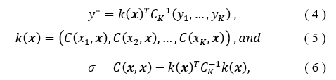
Outpatient clinical data is problematic due to the non-uniform sampling, e.g., time between clinic visits or laboratory tests is not uniform. Additionally, the type of clinical information collected may vary between visits and between patients, e.g., different blood tests may be ordered during each visit or not at all for a given patient. The non-uniformity can be observed in Figure 1 as each set of observations is for a different patient and presents a unique distributions of observations.
A prognosis is formed with respect to a reference time point. For example, predicting if a patient has a LOS of two years requires establishing a reference point from which to count the two years. We establish the three reference points, t, t*1, and t*2 as the basis of the LOS prediction. For each patient, the reference time point t is set when the first type of observation ceases being measured (see Figure 1C). This point was selected to minimize extrapolation errors and dealing with missing data. To avoid bias (t coincides with an observation), t*1 and t*2 are selected at random from a range about t, with t*1 [t-15, t+5 ] selected from the range of 15 days further from death to 5 days closer to death and t*2 [t-28, t+14].
The reference points t* are used in forming the data repre-sentation. The evaluation of the LOS prediction is based on the reference points, t*1 and t*2
3.2. Data Representation
Three representations of the patient clinical observations are considered: clinical data sample values, difference trends, and splines. A fourth type of data representation that of numeric occurrences is used for the counts of medical treatments which
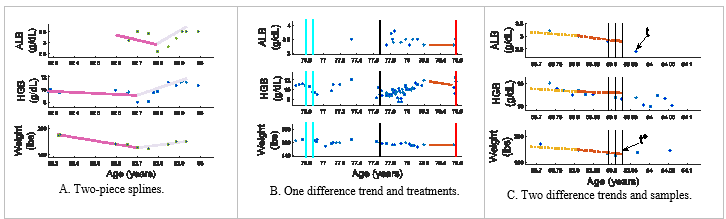 Figure 1 Sample patient data is illustrated with the clinical observations of ALB, HGB and weight (top, middle, and bottom axes). The vertical lines show administered treatments: solid (cyan) – erythropoietin, dashed (black) – blood transfusion, and dot-dash (red) – chemotherapy [1].
the patient experiences. In the data set, these counts include blood transfusion, two different erythropoietins, and chemotherapy. The numeric occurrences (number of treatments) are based in native units prior to standardization.
A patient’s clinical values are estimated at uniform intervals for ALB, HGB, and WT at t* then back at an interval of 7 or 14 days. An example is shown in Figure 1C, where vertical lines represent where the clinical data samples are to be estimated at time t*, t* – 7, and t* – 14 (a sample spacing of 7 days). Cubic splines were utilized to obtain values at the sample times between clinical observations for input to predict LOS by evaluated the splines at the times that the samples were desired. These values are standardized as inputs to the model.
A difference trend (Diffs) describes the observed behavior as increasing, decreasing or stable via a difference between values for ALB, HGB, and WT. Two versions are considered. First, one difference values (1 Diffs) are calculated between values at t*and 90 days earlier, t*-90 (note, the values may be predicted, as a sample may not have been collected at this exact time interval); see Figure 1B. Alternatively, two trends (2 Diffs) are found, from t* back 45 days, then from this point back an additional 45 days; also, shown in Figure 1C).
Finally, splines are used to describe the behavior of the observations. A two-piece second order spline is used to fit the entire observation period for ALB, HGB, and WT observations for a patient (unlike the difference trend which has a recent specified period of consideration); see Figure 1A. The splines’ slope coefficient is discretized and used as input to predict LOS.
In summary, the predictors for prognosis include the number of treatments and the following options to consider in the evaluation: 0-5 patient clinical sample values; 1, 2, or no difference trends; and inclusion or not of spline coefficients.
3.3. Length of Survival (LOS) Prediction via Regression
The problem of regression is a supervised learning technique that aims to develop a model to map an input to an output . The assigned output is a prediction of a continuous quantity or numerical value.
- Linear and Quadratic Regression
In linear regression, the objective of determining the numerical result of is found through a linear model,
![]() where is the input and is the weight that fits the model, that for a linear model is the slope. The parameter is the offset or bias parameter to adjust the fit. The parameters in this case are chosen based on the minimization of the error when fitting with the training set.
where is the input and is the weight that fits the model, that for a linear model is the slope. The parameter is the offset or bias parameter to adjust the fit. The parameters in this case are chosen based on the minimization of the error when fitting with the training set.
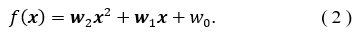
Similar to the linear regression, quadratic regression determines a numerical outcome but from a higher order model,
 3.3.2 Gaussian Process Regression
With a Gaussian Process (GP), the inputs are treated as a set of random variables and incorporated with a covariance function to determine a probabilistic outcome of the regression value [20]. The model is defined by the mean and the covariance functions. Given the K input pairs , the GP regression model summarizes, assuming a zero mean, to [21],
![]() where,
where,
 such that is the covariance matrix evaluated considering the training set inputs and the current input . The covariance matrix has the ability to incorporate a kernel or function to modify the functionality, often smoothing or bring periodicity to the behavior [21]. The correct covariance function can increase when it is in regions which are further away from previous regions of known values, and thus shrinks when near [22]. The constant basis will be used for the function in this analysis.
3.3.3 Support Vector Regression
Support vector regression (SVR) is a kernel based approach to determine the regression output. The regression is a set of linear functions,
![]() that is aimed to have the error minimized through the loss function ε, and where α is the Lagrange multiplier. The support vectors are represented in the term and during the fit process variables w and b are determined, such that w is the weight and b is the offset or bias. To allow for the spread in the values, a slack variable is used, ξi. The objective is then to minimize [23],
that is aimed to have the error minimized through the loss function ε, and where α is the Lagrange multiplier. The support vectors are represented in the term and during the fit process variables w and b are determined, such that w is the weight and b is the offset or bias. To allow for the spread in the values, a slack variable is used, ξi. The objective is then to minimize [23],![]()
when there are l samples. To support this boundary, the slack variable, , must be greater then or equal to zero [23]. In the evaluation the constraint is used to relate the loss and slack variables to the function,
![]() The SVR approach can be extended to allow for the application of kernel which satisfy Mercer’s Condition to be used. In our work, linear and radial basis function kernels will be used.
The SVR approach can be extended to allow for the application of kernel which satisfy Mercer’s Condition to be used. In our work, linear and radial basis function kernels will be used.
4. Experimental Design
There are multiple ways discussed to represent the patient observations: clinical data samples, difference trends, and splines. For example, the number of clinical data samples considered varies from zero to five. The number of difference trends included in the evaluation is zero to two. The spline information is either included or not. All input variables which are not discrete are standardized.
For the evaluation, multiple regression approaches will be used including linear and quadratic regression, GP, and SVR with radial bias function and linear kernels.
For SVR, the linear kernel will be used with the cost parameters from , in addition the radial basis function (RBF) kernel will consider . Each regression model is learned using Matlab 2015b.
In all evaluations, a 10-fold cross evaluation approach was used to train and test. The SVR parameters were selected through a nested cross validation approach. The performance was compared based on the absolute and relative error in the LOS determined for each model evaluated. Statistical p-values from a t-test were used to verify statistical differences or lack thereof in comparing different representation techniques within evaluation methods.
5. Results
The first part of the evaluation was conducted to examine the impact of different number of clinical sample values in the representation (0-5). The data representation also included both behavioral interpretations; namely 1 Diffs and splines. Table 2 shows the best performance was not with more samples but zero or one based on the lowest median relative error, for all but SVR with a linear kernel (although the difference in median relative error between 1, 2, 3, or 5 samples is small). The analysis of the p-values from the t-test showed that the increase in samples had no statistical benefit over less samples for the models. An exception is in the quadratic regression which had a p-value of 0.05 in comparing performance of 1 versus 3 samples. The same analysis was done using t*1 as the reference point, which lead to similar results and conclusions. Because the performance of the models with more samples are not statistically better, then the next part of the evaluation will include only one clinical sample value.
Table 2 Results on t*2 for data representations with 1 Diffs, splines, and different number of clinical sample values with 14d sample spacing.
| Samples | Median Relative Error | ||||
|
SVR- Lin |
SVR-RBF | Linear | Quad | GP | |
| 0 | 0.658 | 0.778 | 0.838 | 1.011 | 0.860 |
| 1 | 0.634 | 0.834 | 0.800 | 1.182 | 0.879 |
| 2 | 0.631 | 0.828 | 0.830 | 1.257 | 0.928 |
| 3 | 0.631 | 0.880 | 0.811 | 1.425 | 0.933 |
| 4 | 0.655 | 0.817 | 0.834 | 1.686 | 0.900 |
| 5 | 0.630 | 0.794 | 0.850 | 2.303 | 0.923 |
Table 3 presents results examining the performance benefit of the inclusion of the behavioral representations namely difference trends (Diffs) and splines. With two exceptions, SVR with the RBF kernel and the quadratic regression, the best performing models contained one behavioral representation. In the various modes of behavioral representation considered, the models did not have any statistical benefit, with p-values greater than 0.1 in most cases. One exception is in quadratic, the model with no splines and no Diffs showed a statistically significant improvement to the model with 2 Diffs and splines with a p-value of 0.014. Similar results were observeved for t*1.
The different regression methodologies show an ability to work with the diversity in the clinical data inputs of the samples to various degrees. The best performing methodology consistently is the SVR with the linear kernel followed by the linear regression approach. The RBF kernel version of the SVR did well with the data, just not as well as the linear kernel method, and the GP was not as successful with the fit but did not have the high degree of variance in the error that was seen with the quadratic regression.
Table 3 Results on t*2 with one clinical sample and different data representations involving the number of Diffs and inclusion of splines.
| # Diffs | Splines | Median Relative Error | ||||
| SVR-Lin | SVR-RBF | Linear | Quad | GP | ||
| 0 | 0 | 0.636 | 0.819 | 0.881 | 0.958 | 0.874 |
| 0 | 1 | 0.649 | 0.844 | 0.800 | 1.064 | 0.870 |
| 1 | 0 | 0.619 | 0.834 | 0.885 | 0.98 | 0.874 |
| 1 | 1 | 0.634 | 0.834 | 0.803 | 1.182 | 0.879 |
| 2 | 0 | 0.720 | 0.868 | 0.866 | 0.979 | 0.878 |
| 2 | 1 | 0.665 | 0.877 | 0.8177 | 1.33 | 0.893 |
Table 4 Best performing regression models. Above the triple line is t*1 and below is t*2.
| Evaluation Method | Data Representation Summary | Median Absolute Error (Days) | Median Relative Error |
| SVR- Linear | 1 Sample, 7 day, 2 Diffs, Splines | 32.48 | 0.625 |
| SVR- RBF | 0 Samples, 2 Diffs, Splines | 31.48 | 0.640 |
| Linear Regression | 3 Samples, 7 day, 2 Diffs, Splines | 51.19 | 0.765 |
| Quad Regression | 1 Sample 14 day, No Diffs, No Splines | 53.05 | 0.800 |
| Gaussian Proc. | 0 Samples, 2 Diffs, Splines | 52.81 | 0.822 |
| SVR- Linear | 1 Sample, 1 Diffs, No Splines | 31.35 | 0.619 |
| SVR- RBF | 0 Samples, 1 Diffs, Splines | 41.60 | 0.752 |
| Linear Regression | 1 Sample, 14 day, No Diffs, Splines | 50.27 | 0.800 |
| Quad Regression | 0 Samples, No Diffs, Splines | 56.05 | 0.889 |
| Gaussian Proc. | 1 Sample, 7 Day, No Diffs, Splines | 53.37 | 0.852 |
The best performing models for each regression methodology is seen in Table 4. These models overall have the best performance with one behavioral representation included with either zero or one sample included. There are a couple cases that the performance was best with multiple behavioral representation included (both Diffs and Splines), and one case with more than one sample being beneficial based on the lower median relative errors.
In Table 4, the median absolute error was also reported. However, it may be a deceiving measure since for each patient the same amount of absolute error may hold more meaning to some cases then other (e.g., an error of 30 days for a patient surviving 40 days versus 180 days). Therefore, to help controlf for each patient’s LOS, the relative error has been reported and used to compare representations and methods. Overall, the best performance in the absolute error was also seen with the SVR methods using this representation approach.
6. Conclusion
The inclusion of more clinical sample values does not provide a statistically significant improvement in the prognostic performance, measured as a reduction in relative error, using regression methodologies. What does help improve the ability to determine a prognosis is the inclusion of behavioral repre-sentations and the selection of appropriate regression methods, like the SVR method used here. While regression and classification are not directly comparable, the original results of benefits from the behavioral representations have held true with prior work. There are several future directions for this work with respect to the data representation. For example, rather than use sampling with interpolation, an alternative would be to consider dimensionality reduction techniques to reduce the need for samples and behavioral representations.
Conflict of Interest
The authors declare no conflict of interest.
Acknowledgment
The authors thank EMOL for providing the patient data for this work.
- J. Winikus and L. E. Brown, “Representation and incorporation of clinical information in outpatient oncology prognosis using Bayesian networks and Naïve Bayes,” in IEEE International Conference on Electro Information Technology (EIT), 2016.
- American Cancer Society, “Cancer facts and figures 2016,” 2016. [Online]. Available: http://www.cancer.org/acs/groups/content/@research/docum ents/document/acspc-047079.pdf.
- A. Vellido and P. J. Lisboa, “Neural networks and other machine learning methods in cancer research,” in Comput. Amb. Intel., 964–971 (2007).
- B. Sierra and P. Larranaga, “Predicting survival in malignant skin melanoma using Bayesian networks,” Artificial Intel. Medicine, 14: 215-230 (1998).
- J. Hayward, S. A. Alvarez, C. Ruiz, M. Sullivan, J. Tseng and G. Whaen, “Machine learning of clinical performance in pancreatic cancer database,” Artificial Intelligence in Medicine, 49: 187-195 (2010).
- L. Karamitopoulos and G. Evangelidis, “Current trends in time series representation,” in Proc. 11th Panhellenic Conference on Informatics, 2007.
- I. Batal, L. Sacchi, R. Bellazzi and M. Hauskrecht, “A temporal abstraction framework for classifying clinical temporal data,” in AMIA Annual Symposium Proceedings, 2009.
- I. Batal, H. Valizadegan, G. F. Cooper and M. Hauskrecht, “A pattern mining approach for classifying multivariate temporal data,” in IEEE Int Conf Bioinformatics Biomed, 2011.
- Y.-J. Tseng, X.-O. Ping, J.-D. Liang, P.-M. Yang, G.-T. Huang and F. Lai, “Multiple-time-series clinical data processing for classification with merging algorithm and statistical measures,” IEEE J. Biomed. Health Informat., 19(3): 1036-1043 (2015).
- D. R. Cox, “Regression models and life-tables,” J. Royal Statistical Society. Series B (Methodological), 34:187-220 (1972).
- P. Royston, “The lognormal distribution as a model for survival time in cancer, with an emphasis on prognostic factors,” Statistica Neerlandica, 55: 89-104 (2001).
- L. Ohno-Machado, “Modeling medical prognosis: survival analysis techniques,” J. Biomed. Infomat. 34: 428-439 (2001).
- S. Gupta, T. Tran, W. Luo, D. Phung, R. L. Kennedy, A. Broad, D. Campbell, D. Kipp, M. Singh, M. Khasraw, L. Matheson, D. M. Ashley and S. Venkaresh, “Machine-learning prediction of cancer survival: a retrospective study using electronic administrative records and a cancer registry,” BMJ Open, 4(3): (2014).
- W. Kim, K. S. Kim, J. E. Lee, D.-Y. Noh, S.-W. Kim, Y. S. Jung, M. Y. Park and R. W. Park, “Development of novel breast cancer recurrence prediction model using support vector machine,” J. Breast Cancer, 15: 230-238 (2012).
- O. Gevaert, F. D. Smet, D. Timmerman, Y. Moreau and B. D. Moor, “Predicting the prognosis of breast cancer by integrating clinical and microarray data with Bayesian networks,” Bioinformatics, 22(14): e184-e190 (2006).
- B. Gan, C.-H. Zheng and H.-q. Wang, “A survey of pattern classification-based methods for predicting survival time of lung cancer patients,” in Bioinformatics and Biomedicine (BIBM), 2014 IEEE International Conference on, 2014.
- D. Delen, G. Walker and A. Kadam, “Predicting breast cancer survivability: a comparison of three data mining methods,” Artific. Intel. Medi., 34: 113-127 (2005).
- I. Anagnostopoulos, C. Anagnostopoulos, D. Vergados, A. Rouskas and G. Kormentzas, “The Wisconsin breast cancer problem: diagnosis and TTR/DFS time prognosis using probabilistic and generalised regression information classifiers,” Oncology Reports, 15: 975-981 (2006).
- H. Valizadegan, Q. Nguyen and M. Hauskrecht, “Learning classification models from multiple experts,” J. Biomed. Informat., 46(6): 1125-1135 (2013).
- C. E. Rasmussen and C. K. Williams, Guassian processes for machine learning, Cambridge: MIT Press, 2006.
- P. Baldi, Bioinformatics: The machine learning approach, Cambridge: MIT Press, 1998.
- Z. Liu, L. Wu and M. Hauskrecht, “Modeling clinical time series using gaussian process sequences,” in SIAM international conference on data mining, 2013.
- V. N. Vapnik, The nature of statistical learning theory, 2 ed., Springer, 2000.
- E. Alpaydin, Introduction to machine learning, 2 ed., Cambridge: MIT Press, 2010.