

Comparison of three undersampling approaches in computed tomography reconstruction
Introduction
Computed tomography (CT) or cone beam CT (CBCT) are volumetric image tools that have been broadly used for diagnosing diseases or guiding treatments. X-ray radiation exposure associated with them is a clinical concern, especially when they are used in a large population of healthy patients, e.g., in lung cancer screening, or repeatedly used on a patient, e.g., during a long course of image-guided radiotherapy treatment. Over the years, several dose reduction approaches such as tube-current modulation (1-4) and data undersampling (5-10) have been developed. In the context of data undersampling, conventional analytical reconstruction approaches are not fully capable of addressing the missing data issue, yielding artifacts in reconstructed images. In contrast, iterative reconstruction techniques motivated by the recent booming research of compressive sensing (CS) (11,12) are more robust to undersampling and are able to retrieve images with satisfactory quality from undersampled data. A number of regularization methods in CS have been introduced to the CT reconstruction problem, such as total variation (TV) (5-9), tight frame (10), and nonlocal means (13-16), etc.
Another motivation for undersampling is to facilitate rapid data acquisition and imaging. Along with recent advancements in CT technology, for instance energy resolved photon-counting detector (17-19), data size in a CT projection becomes larger and larger. This leads to the challenge to quickly read out acquired data before moving to the next projection measurement. Addressing this issue is especially important for those clinical applications requiring a high temporal resolution, e.g., cardiac imaging. While advanced electronics have been designed to improve readout speed, it is also highly desirable to explore novel directions to reduce projection data size without sacrificing quality of reconstructed CT images.
Within the framework of projection data undersampling, it is a natural question regarding the most effective way of sampling. Let us first consider data acquisition without undersampling. This can be expressed in a simple linear system Pf = g, where P is the projection operator that maps an image f to a number of densely placed projection angles. The undersampling operation corresponds to an operator S that has zero or one in its diagonal elements, yielding a data acquisition system Psf = SPf = Sg = gs. Here Ps denotes the undersampling projection operator and gs the corresponding measurements, a subset of the full data vector g. The mathematical properties of Ps depend on the specific way of sampling, namely the operator S. This in turn governs the difficulty of solving the linear system Psf = gs, namely CT reconstruction. Hence, it is interesting to ask which operator S permits the best image restoration. Generally speaking, this is a difficult question. In this paper, it is our motivation to compare three types of undersampling operations, which we hope to shed some light to this question of interest.
There are two typical undersampling approaches that have been widely discussed in the literature. The first one is view undersampling, as illustrated in Figure 1A. Since CT data acquisition is typically performed in a view-by-view fashion, this view undersampling is straightforward in practice: simply tuning on X-ray exposure in those views of interest. Probably due to this reason, view-undersampling approach is the most widely studied undersampling method in low-dose CT problems (5-10). The second approach is regular ray undersampling, as shown in Figure 1B. While X-ray projections are acquired at all the densely placed angles, the X-ray source is blocked by a blocker that has a periodic pattern. This blocking method was originally proposed to address X-ray scatter contamination problem in CBCT (20,21). The signals measured in the purposely-created blocked areas are assumed to be scatter. By smoothly interpolating them to the open areas, scatter signal can be accurately estimated and then corrected. As missing primary data is an apparent problem in this setup, iterative reconstruction approach was employed to improve reconstructed image quality (22).

There are infinitely many ways of undersampling. While it is a difficult problem to theoretically find the best one, we will perform a comparison study of three different undersampling approaches in this paper. In addition to the aforementioned two methods, the third one that will be investigated is random ray undersampling, i.e., each X-ray line is randomly selected with certain probability, as illustrated in Figure 1C. This is motivated by the advancements in CS, where randomness introduced in a data acquisition process typically helps signal restoration. In the rest of this paper, we will compare the properties of the projection matrices in these three undersampling approaches.
Methods
Singular value decomposition (SVD) of a full projection operator
To present theoretical insights of the CT projection operator, we consider CT projection under parallel projection geometry (Figure 2). The reason for this choice is due to the existence of a closed form SVD of the full projection operator under this geometry. Current CT imaging systems employ fan-beam geometry, as illustrated in Figure 1. While this is different from the parallel-beam geometry, we hope the analysis performed in the parallel-beam geometry here captures some insights in the fan-beam setup. The validity of our analysis is demonstrated to some extent by the agreement with numerical experiments performed under the fan-beam geometry.

Consider a 2D function f(x) defined in a unit circle {x ϵ R2:|x|<1}, a parallel X-ray projection operation to all the directions θ ϵ [0, 2π] maps this function into {s, θ} ϵ [–1, 1] × [0, 2π) through a linear system Pf = g, where P is the full projection operator respect to variables s, θ and x. We use the term “full” to denote the situation in which measurements at the entire projection domain are made. When it comes to undersampling, let us consider a general undersampled projection operator Ps = SP, where S = (s, θ) is the sampling operator. The function value of S at (s, θ) is either 1 or 0 depending on whether the data at the coordinate (s, θ) is sampled or not.
In this paper, one objective is to study SVD forms of different undersampling operators. The motivation to pursue this SVD form comes from its importance in reconstruction. Consider a typical reconstruction problem via the least square approach, i.e., solving f = arg min|Pf–g|2, where P is a general projection operator, either full or undersampled. If P has a SVD form [vi(x), ui(s, θ); σi], the solution to the least square problem is simply 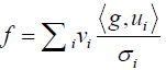 where <., .> denotes a dot product in the Euclidean space. This naturally implies a reconstruction strategy: (I) decomposing the measured projection data g to the basis functions in the projection domain by computing the coefficients <g, ui>; (II) dividing the coefficients by the corresponding singular values σi; and (III) superposing the basic functions vi(x) in the image domain with the modified coefficients. Note that the least square term is a typical choice to ensure data fidelity in many iterative reconstruction approaches.
One particular property of the full projection operator P is that it has an SVD representation [vm,l(x), um,l(s, θ); σm,l] (23) with
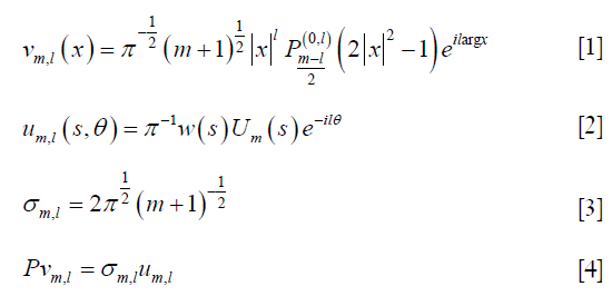
where argx gives angle of the specific points within the unit circle ({x ϵ R2:|x|<1}), 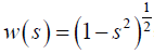 ,
,  is the Jacobi polynomial, and Um(s) is Chebyshev polynomial of second kind with m>0, –m≤l≤m, and m+l being even. l is the index for the projection angle direction and m is the index within a projection. Note that vm,l(x) indicates spherical harmonics which enforces the orthogonality of v as the singular vector in image domain. This decomposition allows reconstructing the image in the full projection case via the aforementioned strategy (24).
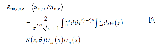
With this basis, we can express the full projection operator P in its matrix representation with matrix elements <um,l, Pvn,k>, m,n>0, |l|≤m, and |k|≤n. Denote the matrix as R. Its matrix element is (23)
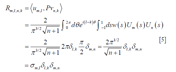
δ is the Kronecker’s delta function. The property of Chebyshev polynomials 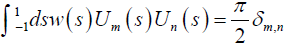 is used here. This implies that R is diagonal (according to its indices given by order of Jacobi polynomials and Chebyshev polynomials) with diagonal elements of σm,l. The matrix R has a block structure in the sense that l and k are block indices corresponding to the projection angle direction and m and n are indices within each block associated with the direction within a projection angle.
The upper limits of these indices are determined by the highest sampling frequency in the corresponding directions. In the continuous setting, the upper limits are infinity. When it comes to a realistic scenario with the number of projections M in the full sampling case, |l|, |k|≤Mang = M/2. Similarly, the finite detector size limits the sampling frequency within a projection. This sets an upper limit of m≤Mdet with Mdet being set to the number of detector elements per projection. Supplementary A presents details on the construction of the matrix R.
SVD of an undersampled projection operator
When it comes to an undersampling problem, presence of the binary undersampling operator S changes the SVD form. For a projection operator Ps, we can write its representation Rs under the basis of vm,l(x) and um,l(s, θ) corresponding to the full projection operator P in the continuous setting. This is analogous to define Rs = UT PsV in the matrix case. This is feasible, since {vm,l(x)} and {um,l(x, θ)} form complete orthogonal basis sets in the image and the projection domains, respectively. Each element of Rs can be expressed as
Rs is no longer diagonal. In the following sections of this paper, we focus on the analysis of three commonly used undersampling techniques: regular view undersampling, regular ray undersampling, and random ray undersampling.
Regular view undersampling
In the case of regular view undersampling, S(s, θ) is unity for  , j = 1, 2, ..., N. The number of projections is N = rM, where r <1 is the radio of undersampling. Hence, we have
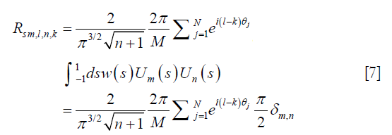
This implies that the matrix elements are nonzero only when the block indices satisfy l–k = tN, tϵ Z, such that
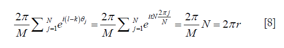
Since –m≤l≤m and m+l even, we can change the notation m→2m+l and n→2n+k. Thus, in the matrix block satisfying l–k = tN, the only nonzero elements should satisfy 2m+l = 2n+k, i.e., m–n = –tN/2, and the matrix element can be obtained by
Apparently, Rs is not a diagonal matrix anymore. Compared to R, the matrix Rs is different due to the existence of off-diagonal blocks at locations satisfying l–k = tN, t ϵ Z. These off-diagonal blocks appear at locations that are at distances tN from the diagonal blocks. An immediate conclusion is that, the smaller N is, the more off-diagonal elements there are, and hence larger difference between Rs and R. This is expected, as a more aggressive undersampling approach changes the system more significantly. On the other hand, when N→∞, the effect of off-diagonal blocks can be ignored, as those blocks are far away from the diagonal. This corresponds to r→1. Comparing Eq. [9]> and Eq. [6], we observe that Rs→R and hence Ps→P as r→1.
Regular ray undersampling
In the case of regular ray undersampling, projections at all angles are acquired, but a periodic undersampling pattern is used within each projection angle. Therefore, S(s, θ) is only a function of s. We consider an example case of S(s) =1, if s ϵ [na, na+b], n ϵ Z, b<a. Here a can be regarded as the period of the regular underampling pattern and b is the width of sampled data within each period. The undersampling ratio r = b/a. We express the matrix of Rs as follows,
This implies that the matrix is of a block diagonal form. For the diagonal block, with a change of notation m→2m+l and n→2n+k,
Compared to the previous view undersampling case that generates a lot of non-zero elements at the off-diagonal blocks of the matrix, regular view undersampling approach only generates off-diagonal elements in the diagonal blocks with l = k.
Random ray undersampling
Random ray under-sampling is a strategy that each X-ray line is sampled with probability r. The resulting underampling pattern gives a sampling function S(s, θ). Again, let us start from the general expression in Eq. [5] but with an exchanged order of the two integrals,
For each fixed s, S(s, θ) is a random variable with binary values depending on θ. For the diagonal blocks l = k,
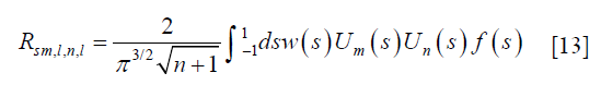
where  is a random valued function with Sj = S(s, θj). The summation follows binomial distribution with mean rM and variance Mr(1–r). It hence follows that f(s) has a mean value of 2πr and variance of
  . For simplicity, we approximate f(s) with a Gaussian random number following the corresponding mean and variance in our numerical evaluation later. The integral over s has to be evaluated numerically.
For the off-diagonal blocks,
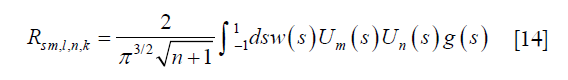
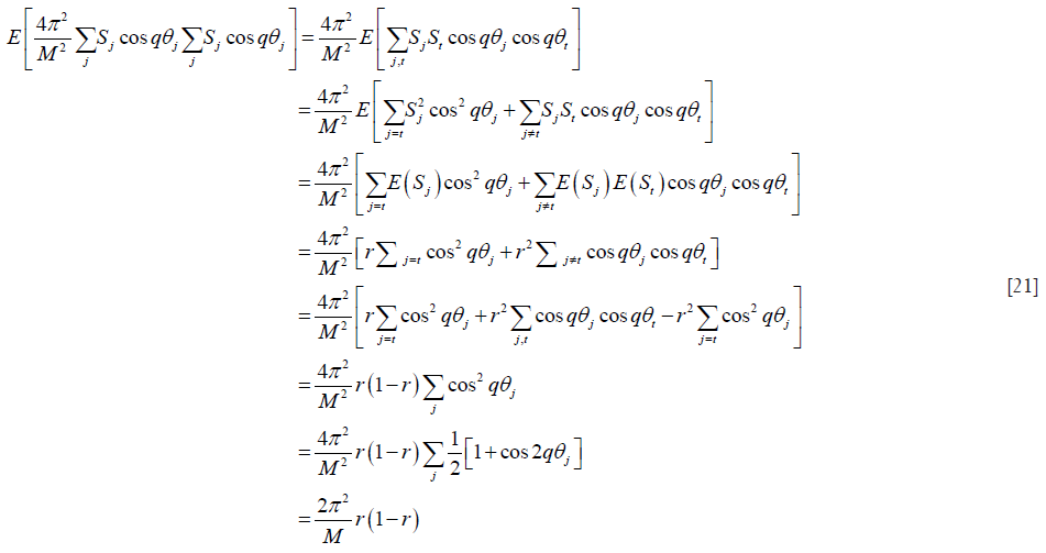
where  is a complex random variable. Its real and imaginary parts are random variables, both with mean zero and variance
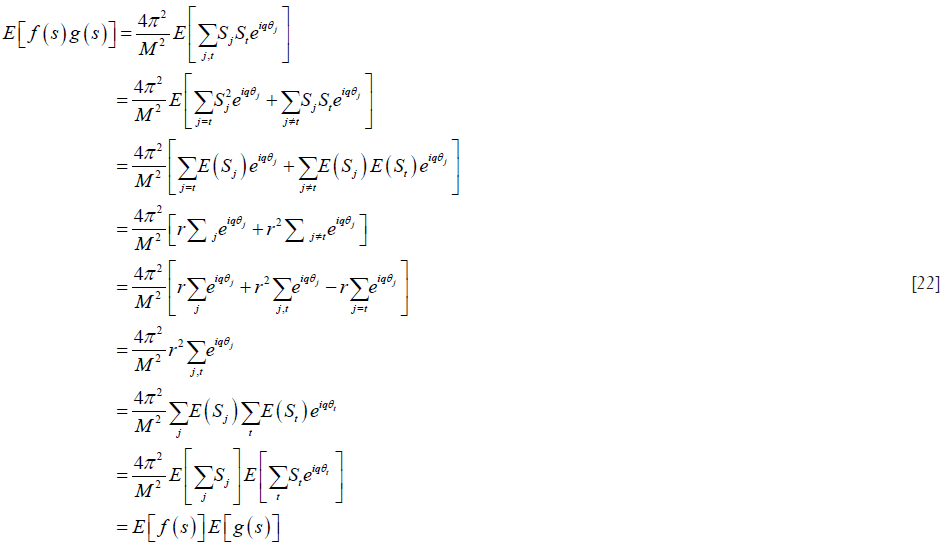
  (Supplementary B). Again, we generate g(s) with its real and imaginary parts sampled according to Gaussian distribution. Then we numerically compute the matrix elements where numerical integration over s is needed. Note that E[f(s)g(s)]=E[f(s)]E[g(s)] (Supplementary C), which implies that f(s) and g(s) are uncorrelated random variables. Hence, we do not consider this correlation when generating off-diagonal block matrix elements.
The above deviation shows that the matrix Rs is dense, although the off-diagonal elements are small, random variables of  , compared to the diagonal elements that are of order 1. The impact of randomness is reflected by the existence of these small off-diagonal matrix elements. There are two special cases to consider: (I) In the limit M→∞, all the off-diagonal elements
  and the diagonal elements are
  . Comparing with Eq. [5], it follows
  . For a real case with a finite but large number of projections, Rs~rR; (II) in the case of r→1, the variance of all the matrix elements approaches 0, and Rs→R as expected.
Numerical SVD
To perform numerical SVD, we consider the discrete case with the projection operator represented using matrix. For each undersampling case, we generate the corresponding matrix representation Rs. All the matrices have the same structure, as shown in Supplementary A. We set M = 2Mang = 200 and Mdet = 250 in our numerical experiments. These parameters are smaller than the actual number of projections and detectors per projection in a real case. However, further increase these values will lead to matrices that are too large to handle. We think the parameter values are large enough to capture properties of a real case. For each matrix, we perform numerical SVD to find matrices W and X, such that Rs = XΛsWT, where Λs is a diagonal matrix with diagonal entries λsi being the singular values of Rs. We would like to remark on the following issues. In the case of regular ray undersampling, the matrix Rs is block diagonalized. Hence, we can perform SVD on each block individually, which is computationally less challenging compared to other cases.
After performing SVD, we first compare singular value spectra in different cases. Particularly, we examine  , where |·|* denotes the matrix nuclear norm. At the continuum limit, |P|* = |R|* and |Ps|* = |Rs|*. Hence,
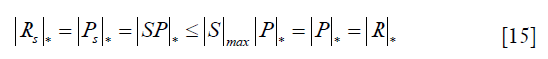
where  gives the largest singular value of X. This implies that μ≤1. For a real discrete case, there is no guarantee that μ≤1. But we expect this still holds in the regime of large Mang and Mdet. We use μ to represent perturbation of the undersampling operation on the full projection case. The smaller μ is, the more dramatically the matrix Rs is altered from R and hence so is Ps compared to P. From reconstruction point of view, it is desired to have a projection operator Ps close to the matrix P to maintain its properties, which means Rs should be also close to R.
The second quantity we examine is matrix rank ratio defined as 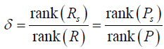 . As the undersampling is taken, it is expected that matrix rank is reduced. A large δ value indicates less rank reduction caused by undersampling, which is a favorable property for solving a linear equation, e.g., in the reconstruction problem.
The third quantity of interest is 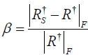 , where
  is Moore-Penrose pseudoinverse of a matrix X. When we consider least square reconstruction problem for Pf = g, the solution is
  . Since
  , the quantity β characterizes the deviation of the least square solution in the undersampled case from the full projection case. In terms of computation,
where tr is matrix trace. For the last term, with numerical SVD of the matrix Rs = XΛsWT, it is easily to show that  , where Σ is a diagonal matrix formed by the singular values of R. Hence, β can be evaluated numerically.
In addition, we compare left singular vectors of Ps that serve as the basis functions in the image domain for the reconstructed CT image. Specifically, with the matrix W in the numerical SVD form Rs = XΛsWT, we compute vsi(x) = ΣjWi,jvj(x). Here vj(x) is the left singular vector of the full projection operator P, whose expression is given in Eqs. [1-4].
CT reconstruction experiment
We perform CT reconstruction experiments aiming at comparing reconstructed image quality among different undersampling approaches at the same undersampling ratio. The Forbild head phantom with a resolution of 256×256 pixels is used. Forward fan-beam projection of the phantom is computed at M =360 equiangular projection angles covering the 2π range. Within each projection, 384 equiangular rays are sampled.
For the regular view undersampling case with a given undersampling ratio r≤1, we compute the number of projections rM and selected this number of equally spaced projection views. For the regular ray undersampling case, within each projection for each consecutive a rays, we selected b=2 rays, such that the ratio  . For the random ray undersampling case, each ray was selected in a random fashion with a probability of r. Once the rays for an undersampling case are selected, projection data gs corresponding to these selected rays are extracted from the already-computed full projection data. Correspondingly, the rows in the system matrix A are selected to form the system matrix As for the undersampled case.
We study two reconstruction models. The first model is a simple least-square model which can be formulated as a quadratic optimization problem
The global optimal solution of this model can be obtained by seeking for f* satisfying  , which can be solved by an iterative linear solver such as conjugate gradient (CG) method. The solution to this problem is directly connected to the SVD form of the system matrix.
The second reconstruction model is based on TV regularization, which solves an optimization problem
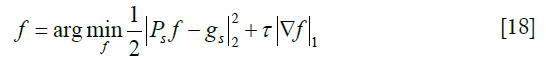
where τ is a parameter that controls the relative contributions of the two terms in the objective function. This parameter is manually selected in each case for the best image quality.
The optimization problem is solved using the Split-Bregman method (25,26) which has been proved to be equivalent to alternating direction method with multiplier (ADMM) (27,28). We study this model for two reasons. First, in the TV method, we expect the least square term produces the underlying structure of an image, and the TV term regularizes the image and removes image artifacts. Hence, the image quality is largely determined by the projection operator properties. Second, the regularized method can produce images with much improved image quality compared to the non-regularized least square method. It is a meaningful study on the performance of the state-of-the-art TV-method in the three undersampling contexts.
Results
Comparison of projection matrices
μ, δ, and β calculated at different undersampling ratios are shown in Figure 3. μ of the random ray undersampling case is the highest among all the three cases. This implies that for a given undersampling ratio, the random ray undersampling preserves the most information. The random ray undersampling approach maintains the same rank as the representation of full projection, whereas the other two operators have substantially reduced rank in the regime with a low undersampling ratio. Moreover, the random undersampling also achieved the lowest β value, implying its advantages in pseudo-inverse calculations.

Finally, the comparison of left singular vectors of Ps in the image domain is depicted in Figure 4. For a fair comparison, we select singular vectors in different cases such that they have approximately similar singular values. The singular vector for the full matrix appeared as a ring pattern. As can be seen from vm,l(x) in Eqs. [1-4], the function amplitude only depends on the radius. The phase angle variation leads to changes of image intensities in real and imaginary parts on a ring. For the regular view undersampling, the off-diagonal elements couple singular modes along the angular directions, breaking this ring pattern. In the regular view undersampling case, the matrix elements couple between modes with in each projection view, leading to strong oscillations along the radial direction. This is reflected as more obvious ring patterns in the singular vector. Finally, although there are off-diagonal elements coupling both the angular and the radial directions in the random ray undersampling case, since these elements are small, they almost have no impact on the singular vector image.

CT reconstruction
After presenting properties of the three different projection operators, we examine how they influence the result of CT reconstruction. All the experiments are performed at a given undersampling ratio of r=0.15. The result of the least-square model in Eq. [14] is given in Figure 5. Without any spatial regularization in the reconstruction model, artifacts are quite obvious in all the three cases, but appearing with different patterns. It is easy to see the severe ring artifacts in the regular ray undersampling case, while serious streak artifacts can be observed in the image under the regular view undersampling. The artifacts in the random ray undersampling case are more noise-like and do not contain a very strong pattern.

Reconstruction results for the TV-based model are presented in Figure 6. The regularization parameter τ for each undersampling scheme was manually tuned for the best reconstruction quality. The ground truth phantom is displayed in Figure 6A1,B1 in two display windows. The use of a narrow window allows visualization of several low contrast objects that are challenging for the reconstruction problem. While all the reconstruction results are visually close to the ground truth in the wide display window, they are dramatically different when being examined in a narrow display window. Specifically, the residual artifacts behaved differently among undersampling cases. As having been commonly observed in many other previous studies, the regular view method generates streak artifacts. The regular ray undersampling gives rise to ring artifacts, which can be ascribed to the strong ring pattern in the singular vectors, e.g., in Figure 4C. In contrast, the random ray approach gives an artifact that appeared as noise. In addition, Figure 6C provides a comparison of line profiles along the line indicated by arrow 4 in Figure 6B1. The zoom-in part demonstrates that the line profile in the random ray undersampling case is closest to that of the ground truth image. Quantitatively speaking, random ray undersampling approach achieved the highest peak signal-to-noise ratio (PSNR) value among all the cases. Figure 6D plots the residual error  as a function of undersampling ratio r. The vertical axis is drawn in the logarithmic scale. Among the three cases, the curve for the random ray undersampling approach stayed at the bottom, indicating the better operator properties in this approach for the CT reconstruction problem.

Discussion
In this paper, we have studied and compared properties of three undersampling operators in CT reconstruction: regular view undersampling, regular ray undersampling, and random ray undersampling. By representing the operators under the basis of singular vectors of the full projection operator, we were able to numerically generate matrices for each case and perform SVD to investigate their properties. It was found that, for a given undersampling ratio, the random ray undersampling approach preserves the properties of the full projection operator better than the other two approaches. This translates to the advantages of reconstructing a CT image at a lower error. Numerical experiments performed on a Forbild phantom demonstrated this fact.
Given the theoretical advantages of random undersampling projection operator, an immediate question is how to realize such a method in a CT or CBCT system. Here we propose two methods. In a CT system, a blocking device similar to the binary multi-leaf collimator used in a Tomotherapy machine could be employed. With a control signal that randomly moves in or out each leaf, random projection data could be acquired. In fact, fluence field modulation has been proposed and investigated in CT reconstruction regime (29,30). Such an idea has been realized on the Tomotherapy machine recently (31). The proposed random sampling approach generally belongs to the fluence field modulation regime, and is hence expected to be achievable in a similar fashion. In CBCT system, modulating fluence of individual pixel is more challenging. Motivated by the beam blocking idea for CBCT scatter estimation, we propose here a rotating block design. Specifically, a blocker with a random blocking pattern (Figure 7) is inserted between the X-ray source and the patient (not drawn). It rotates during CBCT data acquisition under the control of a motor, yielding randomly blocked projections with the blocking pattern varying among projections. One step further, it would be interesting to apply the random projection technique to alternative CT platforms, such as inverse geometry CT system (32-34) which allows reducing of data storage and imaging dose while the time efficiency of CT imaging is boosted.

Main motivation of this study is to introduce randomness in CT data acquisition, in the hope that it would lead to a system matrix that has better numerical properties than the widely used view undersampling or regular ray undersampling methods. Another advantage of it in the CBCT problem is the feasibility for measurement-based scatter estimation and removal. X-ray scatter is the main data contamination factor in CBCT, which degrades accuracy of reconstructed CBCT intensity as well as image contrast. Among many existing methods for scatter estimation and removal, beam blocker-based methods have demonstrated their great potential (20,21). Yet one challenge encountered here was the missing of primary data due to beam blocking. The random undersampling proposed in this paper is compatible with the beam blocker-based scatter removal. With randomly blocked X-ray, the shadow area allows scatter measurement as in the existing approaches. The randomness in data sampling preserves the properties of the projection matrix, permitting high quality CBCT reconstruction. Feasibility for this idea is currently an ongoing study in our group.
One limitation of the current study is that we used parallel-beam geometry for theoretical analysis but fan-beam geometry for numerical studies. Fan-beam geometry is the most widely used CT geometry. But the advantage of parallel-beam system is its nice mathematical property, especially the explicit formula for SVD, which permits the analysis in this paper. Under the condition of full data acquisition, the two geometries are equivalent, as the projection data can be converted between the two cases via re-binning. However, when it comes to undersampling, the equivalence does not exist anymore. In our study, we hope the analysis performed in the parallel-beam geometry captures some insights in the fan-beam setup. This has been demonstrated to a certain extent by the agreement between results in the numerical studies and the theoretical analysis.
Supplementary
A. Construction of R with finite size
Following the notations in Regular view undersampling, k and l are indices for the angular direction and m and n are those for the direction within a projection. The matrix R has a block structure with block indices l and k, and indices inside each block of m and n (Figure S1). In a realistic scenario, m, n, l and k are all finite with m, n≤Mdet and |l|, |k|≤Mang where Mdet and Mang are upper bounds determined by the maximal sampling frequency of detector and projection angles respectively. The following constraints still remain: a) m, n>0; b) –m≤l≤m and m+l even; and c) –n≤k≤n and n+k even. For simplicity we change the notation m→2m+l and n→2n+k and rewrite the constraints as a) 2m+l>0, 2n+k>0; b) –2m≤l≤2m+l; c) –2n–k≤k≤2n+k. Hence, combine the finite-size limit, we have k, l ϵ[–Mang,..., –1, 0, 1,...,Mang] and

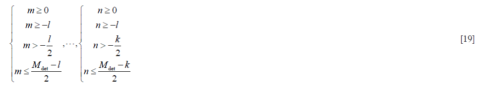
More precisely,  . With these constraints ready, the matrix R has the structure shown in Figure S1 and matrix elements in each block are calculated based on Eq. [5]. Similarly, the matrices for regular view, regular ray and random ray undersampling cases are structured in the same way, with the matrix elements calculated according to Eq. [7], [10], [12], respectively.
B. Mean value and variance of real and imaginary parts of 

For the real part,  , its mean value
Here Σj cosqθj =0 was used. Hence, the variance is
A similar derivation holds for the imaginary part.
Proof of E [f (s) g (s)] = E [f (s)] E [g (s)]
Note that
Acknowledgments
Funding: This work is supported in part by NIH grants R01CA227289, R37CA214639, R21EB021545, and NSF grant DMS-1522786.
Footnote
Conflicts of Interest: The authors have no conflicts of interest to declare.
References
- Jakobs TF, Becker CR, Ohnesorge B, Flohr T, Suess C, Schoepf UJ, Reiser MF. Multislice helical CT of the heart with retrospective ECG gating: reduction of radiation exposure by ECG-controlled tube current modulation. Eur Radiol 2002;12:1081-6. [Crossref] [PubMed]
- Kalra MK, Maher MM, Toth TL, Schmidt B, Westerman BL, Morgan HT, Saini S. Techniques and applications of automatic tube current modulation for CT 1. Radiology 2004;233:649-57. [Crossref] [PubMed]
- Gies M, Kalender WA, Wolf H, Suess C. Dose reduction in CT by anatomically adapted tube current modulation. I. Simulation studies. Med Phys 1999;26:2235-47. [Crossref] [PubMed]
- Kalender WA, Wolf H, Suess C. Dose reduction in CT by anatomically adapted tube current modulation. II. Phantom measurements. Med Phys 1999;26:2248-53. [Crossref] [PubMed]
- Sidky EY, Kao CM, Pan X. Accurate image reconstruction from few-views and limited-angle data in divergent-beam CT. J X-ray Sci Tech 2006;14:119-39.
- Sidky EY, Pan X. Image reconstruction in circular cone-beam computed tomography by constrained, total-variation minimization. Phys Med Biol 2008;53:4777-807. [Crossref] [PubMed]
- Bian J, Siewerdsen JH, Han X, Sidky EY, Prince JL, Pelizzari CA, Pan X. Evaluation of sparse-view reconstruction from flat-panel-detector cone-beam CT. Phys Med Biol 2010;55:6575-99. [Crossref] [PubMed]
- Jia X, Lou Y, Li R, Song WY, Jiang SB. GPU-based Fast Cone Beam CT Reconstruction from Undersampled and Noisy Projection Data via Total Variation. Med Phys 2010;37:1757-60. [Crossref] [PubMed]
- Tian Z, Jia X, Yuan K, Pan T, Jiang SB. Low-dose CT Reconstruction via Edge-preserving Total Variation Regularization. Phys Med Biol 2011;56:5949-67. [Crossref] [PubMed]
- Jia X, Dong B, Lou Y, Jiang SB. GPU-based iterative cone beam CT reconstruction using tight frame regularization. Phys Med Biol 2011;56:3787-807. [Crossref] [PubMed]
- Candes EJ, Tao T. Near-optimal signal recovery from random projections: Universal encoding strategies? IEEE Trans Inf Theory 2006;52:5406-25. [Crossref]
- Donoho DL. Compressed sensing. IEEE Trans Inf Theory 2006;52:1289-306. [Crossref]
- Lou YF, Zhang XQ, Osher S, Bertozzi A. Image Recovery via Nonlocal Operators. J Sci Comput 2010;42:185-97. [Crossref]
- Tian Z, Jia X, Dong B, Lou Y, Jiang SB. Low-dose 4DCT reconstruction via temporal nonlocal means. Med Phys 2011;38:1359-65. [Crossref] [PubMed]
- Jia X, Tian Z, Lou Y, Sonke JJ, Jiang SB. Four-dimensional cone beam CT reconstruction and enhancement using a temporal nonlocal means method. Med Phys 2012;39:5592-602. [Crossref] [PubMed]
- Li B, Shen C, Chi Y, Yang M, Lou Y, Zhou L, Jia X. Multienergy Cone-Beam Computed Tomography Reconstruction with a Spatial Spectral Nonlocal Means Algorithm. SIAM J Imaging Sci 2018;11:1205-29. [Crossref] [PubMed]
- Pelc NJ. Recent and Future Directions in CT Imaging. Ann Biomed Eng 2014;42:260-8. [Crossref] [PubMed]
- Bennett JR, Opie AM, Xu Q, Yu H, Walsh M, Butler A, Butler P, Cao G, Mohs A, Wang G. Hybrid Spectral Micro-CT: System Design, Implementation, and Preliminary Results. IEEE Trans Biomed Eng 2014;61:246-53. [Crossref] [PubMed]
- Cho HM, Barber WC, Ding H, Iwanczyk JS, Molloi S. Characteristic performance evaluation of a photon counting Si strip detector for low dose spectral breast CT imaging. Med Phys 2014;41:091903. [Crossref] [PubMed]
- Zhu L, Xie YQ, Wang J, Xing L. Scatter correction for cone-beam CT in radiation therapy. Med Phys 2009;36:2258-68. [Crossref] [PubMed]
- Zhu L, Bennett NR, Fahrig R. Scatter Correction Method for X-ray CT Using Primary Modulation: Theory and Preliminary Results. IEEE Trans Med Imaging 2006;25:1573-87. [Crossref] [PubMed]
- Dong X, Petrongolo M, Niu T, Zhu L. Low-dose and scatter-free cone-beam CT imaging using a stationary beam blocker in a single scan: phantom studies. Comput Math Methods Med 2013;2013:637614. [Crossref] [PubMed]
- Natterer F. The Mathematics of Computerized Tomography. Society for Industrial and Applied Mathematics, 2001.
- Bortfeld T, Oelfke U. Fast and exact 2D image reconstruction by means of Chebyshev decomposition and backprojection. Phys Med Biol 1999;44:1105-20. [Crossref] [PubMed]
- Cai JF, Osher S, Shen Z. Split Bregman methods and frame based image restoration. SIAM J Multiscale Model Simul 2009;8:337-69. [Crossref]
- Goldstein T, Osher S. The Split Bregman Method for L1-Regularized Problems. SIAM J Imaging Sci 2009;2:323-43. [Crossref]
- Glowinski R, Le Tallec P. Augmented Lagrangian and operator-splitting methods in nonlinear mechanics. SIAM, 1989.
- Glowinski R, Marroco A. Sur l'approximation, par éléments finis d'ordre un, et la résolution, par pénalisation-dualité d'une classe de problèmes de Dirichlet non linéaires. Revue française d'automatique, informatique, recherche opérationnelle Analyse numérique 1975;9:41-76.
- Bartolac S, Graham S, Siewerdsen J, Jaffray D. Fluence field optimization for noise and dose objectives in CT. Med Phys 2011;38:S2-17. [Crossref] [PubMed]
- Bartolac S, Jaffray D. Compensator models for fluence field modulated computed tomography. Med Phys 2013;40:121909. [Crossref] [PubMed]
- Szczykutowicz TP, Hermus J, Geurts M, Smilowitz J. Realization of fluence field modulated CT on a clinical TomoTherapy megavoltage CT system. Phys Med Biol 2015;60:7245-57. [Crossref] [PubMed]
- Schmidt TG, Star-Lack J, Bennett NR, Mazin SR, Solomon EG, Fahrig R, Pelc NJ. A prototype table-top inverse-geometry volumetric CT system. Med Phys 2006;33:1867-78. [Crossref] [PubMed]
- Speidel MA, Wilfley BP, Star-Lack JM, Heanue JA, Van Lysel MS. Scanning-beam digital X-ray (SBDX) technology for interventional and diagnostic cardiac angiography. Med Phys 2006;33:2714-27. [Crossref] [PubMed]
- Speidel MA, Tomkowiak MT, Raval AN, Dunkerley DA, Slagowski JM, Kahn P, Ku J, Funk T. Detector, collimator and real-time reconstructor for a new scanning-beam digital X-ray (SBDX) prototype. Proc SPIE Int Soc Opt Eng 2015. doi: 10.1117/12.2081716. [Crossref]

