Qian He*![]() | Ke Wang
| Ke Wang![]()
© 2023 IIETA. This article is published by IIETA and is licensed under the CC BY 4.0 license (http://creativecommons.org/licenses/by/4.0/).
OPEN ACCESS
Positron Emission Tomography (PET) holds substantial promise in biomedical research and clinical diagnostics. Nonetheless, PET imaging's constraints, typified by deficient sampling and considerable noise interference, often result in the production of inferior quality reconstructed images. These shortcomings can potentially undermine the clinical utility of the modality. To address this issue, this study introduces a novel image reconstruction algorithm underpinned by Bayesian theory that incorporates the total variation model and the median root prior (MRP) algorithm. The iterative resolution process of the algorithm comprises two stages. Initially, the MRP algorithm is employed for image reconstruction. Subsequently, the total variation model is applied to attenuate noise within the reconstructed image. Simulation outcomes reveal that the proposed algorithm effectively mitigates Poisson noise while preserving critical image details, such as edges. When contrasted with traditional reconstruction algorithms, the proposed approach enhances both the precision and reliability of PET imaging markedly. Thus, the algorithm carries significant potential for clinical application and could substantially improve the quality of PET imaging.
Bayesian image reconstruction, PET, total variation model, median root prior, Poisson noise suppression
Positron Emission Tomography (PET), a pioneering imaging technology, has found extensive application in clinical settings alongside Magnetic Resonance Imaging (MRI) and Computed Tomography (CT). Utilized widely for an array of tasks - including tumor cell detection, heart disease diagnosis, neurological and mental disease diagnostics, and the facilitation of new drug development [1] - the influence of PET is substantial. Nevertheless, the efficacy of PET imaging is often hampered by various factors, from imaging duration and radioisotope distribution to statistical counting errors, leading to issues such as reduced resolution and noise pollution [2]. These challenges can profoundly affect early disease detection and clinical diagnostics, underscoring the necessity of enhancing PET imaging quality and accuracy. Consequently, this has become a focal point of contemporary research.
A traditional PET image reconstruction algorithm, the maximum-likelihood expectation-maximization (MLEM) algorithm, takes into consideration the observed data's statistical and physical properties for image reconstruction [3]. Compared to the filtered back-projection (FBP) algorithm, the MLEM algorithm generates images with superior resolution and noise characteristics. However, a significant drawback of the MLEM algorithm is the potential degradation of the reconstructed image's quality when the projection data presents substantial statistical noise. The image quality may not improve with an increased number of iterations and could even deteriorate after a certain number of iterations [4]. This problem can be counteracted by introducing a regularization term into the iterative updating process of the image, limiting the image solution to a regularization space. In PET, this method is often referred to as the Bayesian image reconstruction algorithm [5, 6]. As a widely adopted image reconstruction algorithm, it manages image noise and uncertainty by incorporating prior information, while preserving image details and texture information to achieve more realistic and accurate image reconstruction results [7-9].
Research on PET image reconstruction algorithms based on the total variation (TV) model has shown some advancements [10, 11]. Several studies have enhanced and expanded the total variation model by adding regularization terms, integrating scale space theory, and utilizing optimization algorithms, achieving promising results on various datasets [12, 13]. However, to accommodate clinical needs more effectively, further research is required to improve image resolution, noise suppression ability, and the reliability and applicability of the algorithm.
By integrating the total variation model into the median root prior (MRP) algorithm, a novel image reconstruction algorithm based on Bayesian theory, termed the MRP-PMTV algorithm, has been developed. This algorithm maintains image details and texture while demonstrating an effective noise suppression ability and image resolution. At every iterative step, the MRP algorithm reconstructs the image, and the PMTV model is used to suppress noise. The ensuing discussion delves into the technical intricacies and application advantages of the algorithm, encompassing aspects such as the algorithm principle, implementation process, and performance evaluation. The feasibility and reliability of the novel algorithm have been corroborated through experimental data, providing a foundation for further enhancement of PET imaging quality and accuracy.
In the context of PET, the Bayesian formula can be articulated as:
$p(f|g)=\frac{p(g|f)p(f)}{p(g)},$ (1)
where, p(g|f) represents the likelihood function, p(f) signifies the prior image distribution density, and p(g) denotes the prior projection data distribution density. By substituting the Gibbs energy function into the maximum a posteriori probability objective function, the subsequent objective function can be derived:
$\Psi (f)=l(f)-\beta U(f).$ (2)
The aforementioned objective function can be solved using the EM algorithm, yielding the following image iteration formula:
$f_{j}^{k+1}=\frac{f_{j}^{k}}{\sum\limits_{i=1}^{N}{{{H}_{ij}}+\beta \frac{\partial }{\partial {{f}_{j}}}U(f)}}\sum\limits_{i=1}^{N}{\frac{{{H}_{ij}}{{g}_{i}}}{\sum\limits_{l=1}^{M}{{{H}_{il}}f_{j}^{k}}}}.$ (3)
Given the local correlation of the energy function U(f), a direct solution for the above formula proves challenging. To simplify the solution process, Green proposed the ordered subsets likelihood (OSL) algorithm, which determines the prior image distribution based on the current pixel’s estimated value [14]. The specific iteration formula is as follows:
$f_{j}^{k+1}=\frac{f_{j}^{k}}{\sum\limits_{i=1}^{N}{{{H}_{ij}}+\beta \frac{\partial }{\partial {{f}_{j}}}U(f)|{{f}^{k}}}}\sum\limits_{i=1}^{N}{\frac{{{H}_{ij}}{{g}_{i}}}{\sum\limits_{l=1}^{M}{{{H}_{il}}f_{j}^{k}}}}.$ (4)
In an influential development, Alenius and colleagues proposed the Median Root Prior (MRP) algorithm [15]. This algorithm substitutes the energy function U(f) in the OSL algorithm with a median filter. The iteration formula for the MRP algorithm is given by:
$f_j^{k+1}=f_j^k \frac{\sum_{i=1}^N H_{i j} \frac{g_i}{\sum_{l=1}^M \,\,\,\,H_{i l} \,\,\,\,f_l^k}}{\sum_{i=1}^N H_{i j}+\beta \frac{f_j^k-\operatorname{Med}\left(f^k, j\right)}{\operatorname{Med}\left(f^k, j\right)}}$, (5)
where, Med(fk, j) characterises the median value in the vicinity of the j pixel in the image fk. The neighborhood size is typically a rectangular space of 3×3 or 5×5 pixels. For the purposes of this discussion, it is stipulated that the neighborhood size in the MRP algorithm is a rectangular space of 3×3 pixels. The β is a Bayesian parameter that sets the weight of the prior, the increase in the value of β corresponds to a stronger denoising capability, while a decrease in the value results in a weaker denoising capability.
The operational mechanism of the MRP algorithm can be exemplified through formula (6), a simplified representation of formula (5):
$f_{M R P}^{k+1}(i)=\frac{1}{1+\beta \frac{f^k_{M R P}\,\,\,\,(i)-\operatorname{Med}\left(f_{M R P}^k, \,\,\,\,i\right)}{\operatorname{Med}\left(f_{M R P}^k, \,\,\,\,i\right)}} \quad f_{M \,\,L \,\,E M}^{k+1}(i)$. (6)
Formula (6) elucidates that each iteration of the MRP algorithm necessitates the calculation of both MLEM coefficients and Bayesian coefficients. The MLEM coefficients are instrumental in image reconstruction, while the Bayesian coefficients play a crucial role in noise suppression within the reconstructed image and in preserving fine structures such as edges. In scenarios where the reconstructed image contains noise (locally non-monotonous), the values of $\operatorname{Med}\left(f_{M R P}^k\,\,, i\right)$ and $f_{M R P}^k(i)$ differ. In this case, the Bayesian coefficient deviates from 0, enabling the suppression of noise in the reconstructed image. Conversely, when the reconstructed image is devoid of noise (locally smooth), the values of $\operatorname{Med}\left(f_{M R P}\,\,\,^k\,\,\,, i\right)$ and $f_{M R P}\,\,\,^k(i)$ are identical. Here, the Bayesian coefficient equals 0, and the MRP algorithm reverts to the MLEM algorithm.
The MRP algorithm, in comparison to traditional counterparts, exhibits advantages of rapid calculation speed and potent noise suppression ability. However, the algorithm's sensitivity to small structures within the image necessitates manual parameter adjustment, and it is susceptible to artifacts [16]. Thus, the selection of the prior model for the PET image reconstruction algorithm should be carried out with specific application scenarios and requirements in mind.
The Median Root Prior (MRP) algorithm demonstrates robust noise suppression abilities and rapid calculation speed, making it a potent tool in PET image reconstruction. However, it is not without its challenges: the sensitivity to small structures within the image necessitates careful manual parameter adjustment and can lead to artifacts [16]. Despite these challenges, the MRP algorithm's advantages make it an invaluable tool in the field of PET image reconstruction. It is essential, however, that the prior model selection for the PET image reconstruction algorithm be carried out with due consideration for specific application scenarios and requirements. This will ensure that the algorithm's full potential is harnessed, thereby enhancing the reliability and accuracy of PET imaging.
In 1992, an influential nonlinear full variation image restoration model, known as the Total Variation (TV) model, was proposed by Rudin, Osher, and Fatemi during their exploration of image denoising issues [17]. In this model, images are characterised within the BV space, and the TV model can be articulated as an optimisation problem with noise constraints, represented by the following equation:
$\begin{align} & \underset{u}{\mathop{\min }}\,\int_{\Omega }{\sqrt{u_{x}^{2}+u_{y}^{2}}}\text{d}x\text{d}y, s.t.\int_{\Omega }{u}\text{d}x\text{d}y=\int_{\Omega }{f}\text{d}x\text{d}y,\frac{1}{\left| \Omega \right|}\int_{\Omega }{(f-u})\text{d}x\text{d}y={{\sigma }^{2}}, \end{align}$ (7)
where, f is the noisy image, while u represents the original image. The symbol Ω denotes an image domain, and |Ω| indicates an area within an image. Given the translation invariance of total variation, the initial constraint in formula (7) is inherently satisfied. Consequently, the TV model can be reduced to the subsequent unconstrained optimization problem:
$\underset{u}{\mathop{\min }}\,\int_{\Omega }{\sqrt{u_{x}^{2}+u_{y}^{2}}+\frac{\lambda }{2}}{{(u-f)}^{2}}\text{d}x\text{d}y,$ (8)
In this formula, $\int_{\Omega} \sqrt{u_x^2+u_y^2} d x d y$ constitutes the regular term of image denoising, and $\int_{\Omega} \frac{\lambda}{2}(u-f)^2$ symbolises the fidelity term of image denoising. The λ is a regularization parameter that influences the model's smoothness. A larger value of λ for places more weight on the fidelity term in the model and reduces the model's capacity to smooth and denoise. Conversely, a smaller value pf λ for enhances the model's ability to smooth and denoise. Ideally, should have a larger value of λ at the edge of the image and a smaller value in the flat area, effectively enabling noise suppression while preserving the edge of the image.
To solve the TV model, the corresponding Euler-Lagrange equation must first be determined. For $w \in C_0^1(\Omega)$, the following is defined:
$\begin{align} & g(\varepsilon )=F(u+\varepsilon w)=\int_{\Omega }{\sqrt{{{\left( {{u}_{x}}+\varepsilon {{w}_{x}} \right)}^{2}}+{{\left( {{u}_{y}}+\varepsilon {{w}_{y}} \right)}^{2}}}}\text{d}\Omega +\frac{\lambda }{2}{{\int_{\Omega }{\left( f-u-\varepsilon w\right)}}^{2}}\text{d}\Omega, \end{align}$ (9)
Suppose g'(0)=0, then:
$\int_{\Omega }{\left[ -\text{div}(\frac{\nabla u}{\left| \nabla u \right|})-\lambda (f-u) \right]}\cdot w\text{d}\Omega =0.$ (10)
According to the arbitrariness of w, it can be known that:
$-\text{div}\left( \frac{\nabla u}{\left| \nabla u \right|} \right)-\lambda (f-u)=0.$ (11)
By introducing the time variable t, the gradient descent method is used to solve. Formula (11) can be transformed into:
$\frac{\partial u}{\partial t}=div\left( \frac{\nabla u}{\left| \nabla u \right|} \right)+\lambda (f-u).$ (12)
In order to avoid |∇u|=0 causing singularity, the parameter ξ>0 is introduced, which can be obtained:
$\frac{\partial u}{\partial t}=\text{div}\left( \frac{\nabla u}{\sqrt{u_{x}^{2}+u_{y}^{2}+\xi }} \right)+\lambda (f-u).$ (13)
Suppose the size of the image u is N×N pixels, let $(\nabla u)_{i, j}=\left(\left((\nabla u)_{i, j}^1\right),\left((\nabla u)_{i, j}^2\right)\right)$, where:
$\begin{aligned} & (\nabla u)_{i, j}^1=\left\{\begin{array}{cc}u_{i+1, j}-u_{i, j}, & i<N, \\ 0, & i=N .\end{array}\right. \\ & (\nabla u)_{i, j}^2=\left\{\begin{array}{cc}u_{i, j+1}-u_{i, j}, & j<N ; \\ 0, & j=N .\end{array}\right.\end{aligned}$ (14)
Formula (13) can be transformed into:
$\frac{u_{n+1}\,\,-u_n}{\Delta t}=\operatorname{div}\left(\frac{\left(\nabla u_n^1, \nabla u_n^2\right)}{\sqrt{u_x^2+u_y^2+\xi}}\right)+\lambda(f-u)$ (15)
Make
$p=\frac{(\nabla u_{n}^{1},\nabla u_{n}^{2})}{\sqrt{u_{x}^{2}+u_{y}^{2}+\xi }}$, ${{p}^{1}}=\frac{\nabla u_{n}^{1}}{\sqrt{u_{x}^{2}+u_{y}^{2}+\xi }}$, ${{p}^{2}}=\frac{\nabla u_{n}^{2}}{\sqrt{u_{x}^{2}+u_{y}^{2}+\xi }}$
Thus,
$\begin{align} & \frac{{{u}_{n+1}}-{{u}_{n}}}{\Delta t}=\text{div}(p)+\lambda (f-u)=\text{div}(({{p}^{1}},{{p}^{2}}))+\lambda (f-u). \end{align}$ (16)
where,
$\begin{aligned} & (\operatorname{div}(p))_{i, j}= \\ & \left\{\begin{array}{cc}p_{i, j}^1-p_{i-1, j}^1, 1<i<N ; \\ p_{i, j}^1, & i=1 ; \\ -p_{i-1, j}^1, & i=N .\end{array}+\left\{\begin{array}{cc}p_{i, j}^2-p_{i, j-1}^2, 1<j<N ; \\ p_{i, j}^2, & j=1 ; \\ -p_{i, j-1}^2, & j=N .\end{array}\right.\right.\end{aligned}$ (17)
To sum up, the discrete formula of the TV model can be expressed as:
${{u}_{n+1}}={{u}_{n}}+\Delta t\left[ \text{div}\left( \frac{\nabla u}{\sqrt{u_{x}^{2}+u_{y}^{2}+\xi }} \right)+\lambda (f-u) \right].$ (18)
The Total Variation (TV) model is renowned for its effective filtration of Gaussian noise, a feature shared with many other image denoising models. However, the model's performance is less than satisfactory in cases where the noise is dominated by signal-related Poisson noise, a common occurrence in images such as radiological ones. To address this limitation, TRIET LE proposed an innovative image denoising algorithm known as the Poisson-modified Total Variation (PMTV) algorithm [18]. This algorithm modifies the data fidelity term in the TV model to filter Poisson noise in the image. The PMTV algorithm can be formulated as the following optimisation problem:
With the introduction of the PMTV algorithm, a novel approach towards the problem of Poisson noise in images, particularly radiological ones, is provided. This represents a significant stride in the field of image denoising, offering a solution to a previously unaddressed issue in the TV model. The PMTV algorithm, with its adapted data fidelity term, shows promise for enhanced noise reduction in images impacted by signal-related Poisson noise.
$\underset{u}{\mathop{\min }}\,\int_{\Omega }{(u-f\lg u)\text{d}x\text{d}y+\beta \int_{\Omega }{\left| \nabla u \right|}}\text{d}x\text{d}y.$ (19)
The Euler lagrange equation corresponding to the above formula is:
$0=\text{div}(\frac{\nabla u}{\left| \nabla u \right|})+\frac{1}{\beta u}(f-u).$ (20)
The distinction between the Poisson-modified Total Variation (PMTV) model and the Total Variation (TV) model lies primarily in the regularization parameter λ=1/(βu). In the PMTV model, the regularization parameter, is adaptive and is related to the signal. This parameter is instrumental in enabling the PMTV model to effectively suppress Poisson noise.
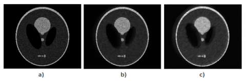
The comparative performance of the PMTV and TV models in filtering Poisson noise is illustrated in Figure 1. From this figure, it is observable that the image processed through the PMTV model exhibits superior smoothness, decreased noise, and enhanced quality. This demonstrates the PMTV model's effectiveness in addressing the limitations of the TV model, specifically in relation to signal-related Poisson noise suppression, thereby making it a potentially potent tool in the field of image denoising.
Figure 1. The filtering effect of PMTV and TV model on Poisson noise: a) Noisy images; b) Noise filtering of TV model; c) Noise filtering of PMTV model
In the process of signal acquisition and image reconstruction of Positron Emission Tomography (PET) images, significant noise, primarily Poisson noise, is generated. This noise can directly impact the accuracy of clinical diagnoses. To address this challenge, a novel PET image reconstruction algorithm has been proposed, which integrates the Penalized Maximum-a-posteriori Total Variation (PMTV) model into the Maximum Likelihood Expectation Maximization (MLEM) algorithm. Based on Bayesian theory, this algorithm is referred to as the MRP-PMTV algorithm. The specific iterative equation is presented as follows:
$f_j^{k+1, l}=f_j^{k, l} \frac{\sum_{i=1}^N H_{i j} \frac{g_i}{\sum_{l=1}^M H_{i l} \,\,,\,f_l^{k, l}}}{\sum_{i=1}^N H_{i j}+\beta \frac{f_j^{k, l}-\operatorname{Med}\left(f^{k, l}\,\,,\,\, j\right)}{\operatorname{Med}\left(f^{k, l}\,,\,\, j\right)}}$ (21)
$u_j^{k+1, l}=f_j^{k+1, l}+\Delta t * \operatorname{div}\left(\frac{\nabla f_j^{k+1, l}}{\sqrt{\left|\nabla f_j^{k+1, l}\,\,\,\,\right|+\xi}}\right)$ (22)
$f_{j}^{k+1,l+1}=u_{j}^{k+1,l}+\Delta t*\lambda (f_{j}^{k+1,l}-u_{j}^{k+1,l}).$ (23)
In these equations, the symbol k represents the number of MLEM algorithm iterations, while symbolizes the number of PMTV model iterations. All other parameters maintain their previous definitions.
The proposed methodology, which incorporates the benefits of the PMTV model, can effectively suppress Poisson noise. Lower-level noise is diffused, and higher-level noise is eliminated by the MRP algorithm. In essence, the PMTV model and MRP algorithm work in tandem, mutually complementing each other to gradually eliminate noise without blurring the image edges.
This proposed method represents a significant advancement in PET image reconstruction, as it offers an effective solution to the challenge of noise in the diagnostic process. Through the integration of the PMTV model and the MRP algorithm, this approach ensures that the accuracy of clinical diagnoses is not compromised due to noise interference. As such, the MRP-PMTV algorithm has the potential to significantly improve the reliability of PET imaging in clinical practice, opening new avenues for patient care and disease management.
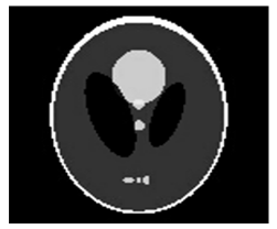
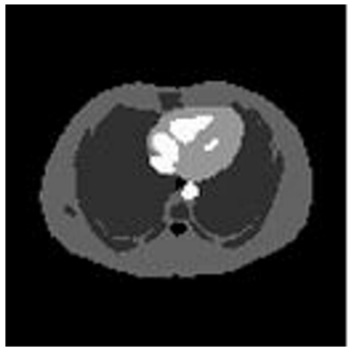
In the conducted simulation experiment, the initial test image was generated computationally, using the Shepp-Logan phantom [19], which has a size of 128×128 pixels. Each pixel within this image falls within the gray value range of 0-255, as demonstrated in Figure 2. The projection parameter is assumed to be 128×128, with 128 projection directions uniformly distributed between 0∼π, and 128 detector pairs aligned in each projection direction. Noise-free observations were generated using formula g=Hf, which in turn were used as the mean of the Poisson variables for the creation of actual noisy projection data. Throughout the simulation experiment, the total number of photon pairs collected approximated 6×10⁵.
Figure 2. Shepp-Logan phantom
The effectiveness of the novel MRP-PMTV algorithm was compared and analyzed against that of traditional MLEM-PMTV, MRP, and MLEM algorithms in the simulation experiment, with the aim of showcasing the superior performance of the new method. To ensure fairness, the iteration number for each algorithm was set to 50, and l was set to 15, following the parameter setting method from the literature [18]. The step size in the MRP-PMTV algorithm Δt was set to 0.1, the regularization parameter was set to 0.3, and the parameter β was set to 0.5. In the MLEM-PMTV algorithm, was set to 0.8, and the regularization parameter was set to 0.3. Within the MRP algorithm, was set to 0.5. Figure 3 presents the reconstructed image of the Shepp-Logan phantom as produced by the four algorithms, while Figure 4 provides a magnified view of a portion of Figure 3.
This simulation experiment serves to demonstrate the efficacy of the proposed MRP-PMTV algorithm in comparison to established methods. The image reconstruction results clearly illustrate the performance of each algorithm, highlighting the advantages of the new method. The carefully controlled parameters and settings ensure a fair and accurate comparison, effectively showcasing the potential of the MRP-PMTV algorithm in real-world applications.
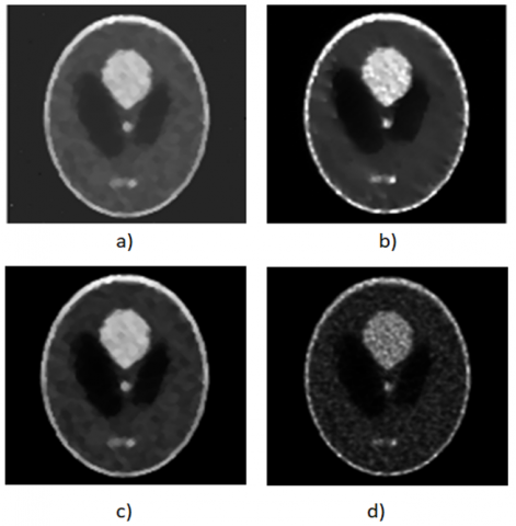
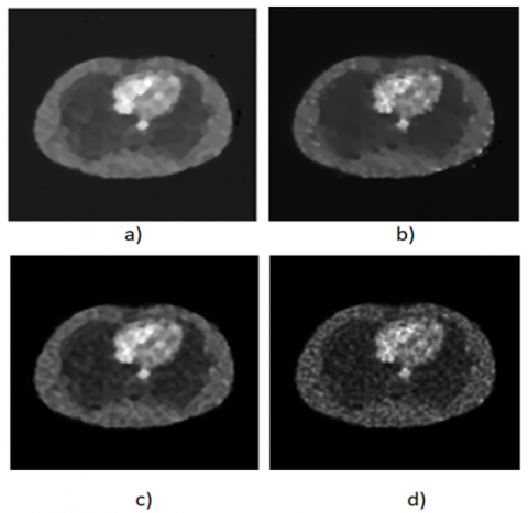
Figure 3. The Shepp-Logan phantom reconstructed by four algorithms: a) MRP-PMTV; b) MLEM-PMTV c) MRP; d) MLEM
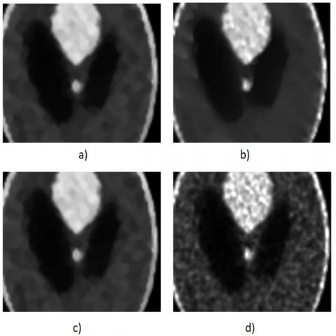
As per the visual evidence provided by Figures 3 and 4, the reconstructed image quality yielded by the MLEM algorithm was found to be inferior. The image was not only characterized by considerable noise and blurred edges, but a substantial loss of crucial information was also observed. Although the MLEM-PMTV and MRP algorithms produced better reconstructed images compared to the MLEM algorithm, the presence of noticeable noise and artifacts remained. Contrarily, the proposed MRP-PMTV algorithm demonstrated superior performance, with the reconstructed image exhibiting less noise and sharper edges. From a subjective visual perspective, the MRP-PMTV algorithm's overall effect was deemed superior.
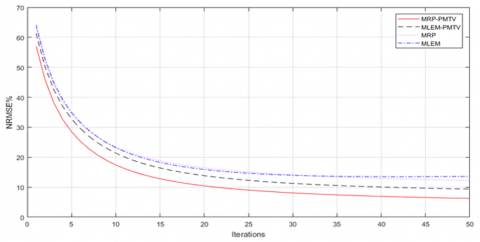
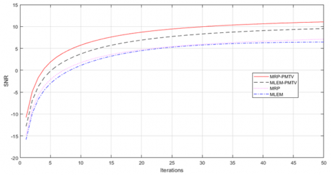
The Normalized Root Mean Square Error (NRMSE) and Signal-to-Noise Ratio (SNR) values of the images were calculated to provide a quantitative measure of the algorithm's effectiveness [20]. Figure 5 illustrates the plot of NRMSE values over the course of iterations for the Shepp-Logan phantoms reconstructed by the four algorithms. As discerned from Figure 5, the lowest NRMSE value was attributed to the novel MRP-PMTV algorithm, indicating its reconstructed image was closest to the original image. Therefore, it can be deduced that the MRP-PMTV algorithm delivered the best reconstruction. Similarly, the SNR graph presented in Figure 6 corroborated these findings.
To further substantiate the effectiveness of the proposed MRP-PMTV algorithm, a thorax phantom was selected as the test model. The thorax phantom model was of a size pixels, with the gray value range for each pixel set between 0-255, as depicted in Figure 7. The projection data was obtained through a method analogous to the previous one, and the total number of photon pairs collected approximated 5.2×10⁵.
The selection of the thorax phantom provided an additional complex test scenario, aiming to further validate the MRP-PMTV algorithm's effectiveness across different imaging challenges. This step of the simulation experiment added robustness to the overall study, ensuring that the proposed algorithm performs consistently across various test models.
Figure 4. Partial enlarged image of Figure 3: a) MRP-PMTV; b) MLEM-PMTV c) MRP; d) MLEM
Figure 5. The plots of NRMSE along with iterations for Shepp-Logan phantoms reconstructed by four algorithms
Figure 6. The plots of SNR along with iterations for Shepp-Logan phantoms reconstructed by four algorithms
Figure 7. Thorax phantom
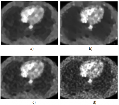
Figure 8. The thorax phantom reconstructed by four algorithms: a) MRP-PMTV; b) MLEM-PMTV c) MRP; d) MLEM
A comparison was drawn between the proposed MRP-PMTV algorithm and three other algorithms: MLEM-PMTV, MRP, and MLEM. In the simulation experiment, the iteration number was uniformly set to 50 across all algorithms, and l was set to 15. For the MRP-PMTV algorithm, the step size Δt was established at 0.1, the regularization parameter was defined as 0.3, and the parameter β was designated at 0.5. In the MLEM-PMTV algorithm, Δt was set to 0.7 and the regularization parameter is set to 0.3, while in the MRP algorithm, β was set to 0.5. The reconstructed images produced by these four algorithms are displayed in Figure 8, with Figure 9 providing a magnified view of a selected region from Figure 8.
Despite the presence of discernible noise in the reconstructed image yielded by the new algorithm, its quality was noticeably superior when juxtaposed with the other three algorithms. The new algorithm's image exhibited the least noise, the most defined edges, and provided the most satisfactory overall visual effect.
Figure 9. Partial enlarged image of Figure 8: a) MRP-PMTV; b) MLEM-PMTV c) MRP; d) MLEM
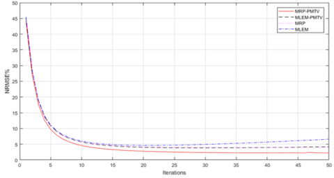
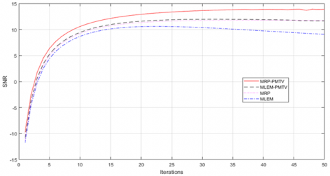
Figures 10 and 11 present the plots of the NRMSE and SNR values, respectively, over the course of iterations for the thorax phantoms reconstructed by the four algorithms. These figures further corroborate the superior performance of the new algorithm over the MLEM-TV, MRP, and MLEM algorithms.
The comprehensive analysis of the reconstructed thorax phantom images, along with the accompanying NRMSE and SNR values, provides a compelling case for the superior performance of the proposed MRP-PMTV algorithm. This section serves to reinforce the effectiveness of the new algorithm under diverse imaging conditions, further validating its potential for real-world applications. It is worth noting that, despite the presence of noise in the images produced by the new algorithm, the overall image quality significantly surpasses those generated by the other algorithms. This highlights the robustness of the MRP-PMTV algorithm in dealing with complex imaging scenarios.
Figure 10. The plots of NRMSE along with iterations for thorax phantoms reconstructed by four algorithms
Figure 11. The plots of SNR along with iterations for thorax phantoms reconstructed by four algorithms
The introduction of the PMTV model into the MRP algorithm has facilitated the formulation of a novel PET image reconstruction algorithm, MRP-PMTV. Experimental outcomes have illuminated the capacity of this new algorithm to adeptly suppress Poisson noise present in the reconstructed image. Furthermore, it has been demonstrated that the algorithm effectively eradicates artifacts and safeguards critical attributes of the image, such as edges. The substantial enhancement in image quality, as evidenced by the experimental results, attests to the feasibility of employing the MRP-PMTV algorithm in PET image reconstruction.
The superiority of the MRP-PMTV algorithm is further underscored when examined against existing algorithms such as MLEM-PMTV, MRP, and MLEM. This was established through quantitative metrics, including Normalized Root Mean Square Error (NRMSE) and Signal-to-Noise Ratio (SNR), and supplemented by visual evaluations. The MRP-PMTV algorithm consistently delivered the lowest NRMSE values and the highest SNR values, signifying its reconstructed images were closest to the original images and exhibited least noise, respectively.
In the wake of these compelling results, the MRP-PMTV algorithm emerges as a promising tool in the realm of PET image reconstruction. The successful suppression of noise, elimination of artifacts, and preservation of critical image information mark a significant leap forward in reconstruction quality. Future research might focus on further optimizing the algorithm parameters and exploring the algorithm's performance in other imaging modalities. The potential impact of these advancements on clinical applications and patient outcomes is indeed exciting and warrants further investigation.
This research was funded by: Scientific research project of Hunan Education Department (Grant No.: 22A0555); Natural science foundation of Hunan Province (Grant No.: 2023JJ50354).
[1] Moehrs, S., Del Guerra, A., Herbert, D.J., Mandelkern, M.A. (2006). A detector head design for small-animal PET with silicon photomultipliers (SiPM). Physics in Medicine & Biology, 51(5): 1113. https://doi.org/10.1088/0031-9155/51/5/004
[2] Reader, A.J., Corda, G., Mehranian, A., da Costa-Luis, C., Ellis, S., Schnabel, J.A. (2020). Deep learning for PET image reconstruction. IEEE Transactions on Radiation and Plasma Medical Sciences, 5(1): 1-25. https://doi.org/10.1109/TRPMS.2020.3014786
[3] Chen, Z.X., Zhang, Q.Y., Zhou, C., Zhang, M.X., Yang, Y.F., Liu, X., Zheng, H.R., Liang, D., Hu, Z.L. (2020). Low-dose CT reconstruction method based on prior information of normal-dose image. Journal of X-ray Science and Technology, 28(6): 1091-1111. https://doi.org/1111. 10.3233/XST-200716
[4] Liu, Z., Ye, H., Liu, H. (2022). Deep-learning-based framework for PET image reconstruction from sinogram domain. Applied Sciences, 12(16): 8118. https://doi.org/10.3390/app12168118
[5] Xie, W.S., Yang, Y.F., Zhou, B. (2014). An ADMM algorithm for second-order TV-based MR image reconstruction. Numerical Algorithms, 67(4): 827-843. https://doi.org/10.1007/s11075-014-9826-z
[6] Schiano Di Cola, V., Mango, D.M., Bottino, A., Andolfo, L., Cuomo, S. (2023). Magnetic resonance imaging enhancement using prior knowledge and a denoising scheme that combines total variation and histogram matching techniques. Frontiers in Applied Mathematics and Statistics, 9: 1041750. https://doi.org/10.3389/fams.2023.1041750
[7] Gou, Y., Li, B., Liu, Z., Yang, S., Peng, X. (2020). Clearer: Multi-scale neural architecture search for image restoration. Advances in Neural Information Processing Systems, 33: 17129-17140.
[8] Li, K., Chandrasekera, T.C., Li, Y., Holland, D.J. (2018). A non-linear reweighted total variation image reconstruction algorithm for electrical capacitance tomography. IEEE Sensors Journal, 18(12): 5049-5057. https://doi.org/10.1109/JSEN.2018.2827318
[9] McGaffin, M.G., Fessler, J.A. (2015). Fast GPU-driven model-based X-ray CT image reconstruction via alternating dual updates. In Proceedings of the International Meeting on Fully 3D Image Reconstruction in Radiology and Nuclear, Medicine, pp. 312-315.
[10] H Srivastava, S., Kumar, G., Mishra, R.K., Kulshrestha, N. (2020). A complex diffusion based modified fuzzy C- means approach for segmentation of ultrasound image in presence of speckle noise for breast cancer detection. Revue d'Intelligence Artificielle, 34(4): 419-427. https://doi.org/10.18280/ria.340406
[11] Khalane, V., Suralkar, S., Bhadade, U. (2020). Image encryption based on matrix factorization. International Journal of Safety and Security Engineering, 10(5): 655-661. https://doi.org/10.18280/ijsse.100510
[12] Jidesh, P., Holla, S. (2018). Non-local total variation regularization models for image restoration. Computers & Electrical Engineering, 67: 114-133. https://doi.org/10.1016/j.compeleceng.2018.03.014
[13] Gong, C., Zeng, L. (2020). Self-guided limited-angle computed tomography reconstruction based on anisotropic relative total variation. IEEE Access, 8: 70465-70476. https://doi.org/10.1109/ACCESS.2020.2985107
[14] Green, P.J. (1990). Bayesian reconstructions from emission tomography data using a modified EM algorithm. IEEE Transactions on Medical Imaging, 9(1): 84-93. https://doi.org/10.1109/42.52985
[15] Alenius, S., Ruotsalainen, U. (1997). Bayesian image reconstruction for emission tomography based on median root prior. European Journal of Nuclear Medicine, 24: 258-265. https://doi.org/10.1007/BF01728761
[16] Xu, J., Zhao, Y., Li, H., Zhang, P. (2019). An image reconstruction model regularized by edge-preserving diffusion and smoothing for limited-angle computed tomography. Inverse Problems, 35(8): 085004. https://doi.org/10.1088/1361-6420/ab08f9
[17] Li, R., Osher, S., Fatemi, E. (1992). Nonlinear total variation based noise removal algorithms. Physica D: Nonlinear Phenomena, 60(1-4): 259-268. https://doi.org/10.1016/0167-2789(92)90242-F
[18] Le, T., Chartrand, R., Asaki, T. J. (2007). A variational approach to reconstructing images corrupted by Poisson noise. Journal of Mathematical Imaging and Vision, 27(3): 257-263. https://doi.org/10.1007/s10851-007-0652-y
[19] Sung, Y., Segars, W.P., Pan, A., Ando, M., Sheppard, C.J., Gupta, R. (2015). Realistic wave-optics simulation of X-ray phase-contrast imaging at a human scale. Scientific Reports, 5(1): 12011. https://doi.org/10.1038/srep12011
[20] Sun, Y., Li, Y., Feng, K. (2022). Improved PCNN polarization image denoising method based on grey wolf algorithm and non-subsampled contourlet transform. Journal of Computational and Cognitive Engineering, 1-11. https://doi.org/10.47852/bonviewJCCE3202943