


Abstract
The distribution of mutational effects on fitness is of fundamental importance for many aspects of evolution. We develop two methods for characterizing the fitness effects of deleterious, nonsynonymous mutations, using polymorphism data from two related species. These methods also provide estimates of the proportion of amino acid substitutions that are selectively favorable, when combined with data on between-species sequence divergence. The methods are applicable to species with different effective population sizes, but that share the same distribution of mutational effects. The first, simpler, method assumes that diversity for all nonneutral mutations is given by the value under mutation-selection balance, while the second method allows for stronger effects of genetic drift and yields estimates of the parameters of the probability distribution of mutational effects. We apply these methods to data on populations of Drosophila miranda and D. pseudoobscura and find evidence for the presence of deleterious nonsynonymous mutations, mostly with small heterozygous selection coefficients (a mean of the order of 10−5 for segregating variants). A leptokurtic gamma distribution of mutational effects with a shape parameter between 0.1 and 1 can explain observed diversities, in the absence of a separate class of completely neutral nonsynonymous mutations. We also describe a simple approximate method for estimating the harmonic mean selection coefficient from diversity data on a single species.
SURVEYS of DNA sequence polymorphisms in many species have revealed substantial variation in the aminoacid sequences of proteins, although the nonsynonymous nucleotide site diversity is usually much less than that for silent variants (Li 1997). This is consistent with the action of purifying selection on protein sequences, removing deleterious amino acid mutations from the population while neutral or nearly neutral silent variants can persist (Kimura 1983; Li 1997). It is clearly important to characterize the distribution of fitness effects of new nonsynonymous mutations. This distribution is relevant to a broad range of problems in evolutionary genetics, and a variety of methods have been used to characterize it, including direct estimates from mutation-accumulation experiments and indirect estimates from comparisons of DNA sequences among related species (Keightley and Eyre-Walker 1999). The extent, nature, and magnitude of selection on amino acid variants are also relevant to understanding the relation between human disease and genetic variation (Sunyaev et al. 2001; Wright et al. 2003).
Several methods have been used to detect purifying selection from data on variability in natural populations and to estimate the parameters describing such selection. An important method was introduced by Sawyer and Hartl (1992), based on the McDonald-Kreitman test (McDonald and Kreitman 1991). It compares the ratio of the number of within-species nonsynonymous polymorphisms to the number of synonymous polymorphisms and the corresponding ratio for fixed differences between a pair of related species. This ratio of ratios is called the “neutrality index” (Rand and Kann 1996). It is expected to be greater than one if there is predominantly purifying selection against nonsynonymous variants, since selection is less effective in reducing the level of polymorphism for deleterious variants than in preventing their fixation (Kimura 1983). This approach can be incorporated into maximum-likelihood or Bayesian methods for estimating Nes, where Ne is the effective population size and s is the selection coefficient against nonsynonymous mutations. The selective effects of mutations are usually assumed to be codominant (in the case of nuclear genes), and constant across sites within a gene (e.g., Nachman 1998; Bustamante et al. 2002). Recent extensions allow for a distribution of selection coefficients at different sites (Piganeau and Eyre-Walker 2003) or varying degrees of dominance (Williamson et al. 2004).
Overall, this method has been more successful in detecting and estimating purifying selection on nonsynonymous variants in mitochondrial genomes than in the nuclear genome (Nachman 1998; Rand and Kann 1998; Weinreich and Rand 2000), with a few exceptions such as Arabidopsis thaliana (Bustamante et al. 2002), Drosophila miranda (Bartolomé et al. 2005), and humans (Bustamante et al. 2005). The fixed selection coefficient model was fitted by Nachman (1998) to 17 animal mitochondrial DNA data sets with neutrality index values >1 and gave Nes estimates predominantly between 1 and 3; Bustamante et al. (2002) estimated Nes on a gene-by-gene basis and obtained a mean value of ∼1 for 12 nuclear genes in A. thaliana (in both cases, Ne is the haploid effective population size, as is appropriate for the ploidy and breeding systems in these cases). A modification of this approach, allowing a normal distribution of Nes values across different genes, was applied to data on D. melanogaster, indicating a mean Nes of ∼3.5 (Sawyer et al. 2003). The fits of a gamma distribution of selection coefficients across individual nonsynonymous sites to animal mitochondrial data sets (Piganeau and Eyre-Walker 2003) gave much larger but noisier estimates of mean Nes.
An alternative approach is to fit the observed frequency spectra of nonsynonymous and silent/synonymous variant frequencies to the distributions expected under mutation-selection-drift equilibrium (Sawyer 1994; Sawyer et al. 1987). Variants of this approach have been developed by Hartl et al. (1994), Akashi (1999), Fay et al. (2001), Bustamante et al. (2003), and Williamson et al. (2004, 2005). Either a fixed given Nes value or a distribution of Nes values across loci is assumed.
These studies have yielded large differences among estimates of the scaled selection parameter Nes (or its arithmetic mean) for nonsynonymous sites under purifying selection, ranging from values of the order of 1 to several hundred, depending on the methods and species used. Varying conclusions about the proportion of sites subject to positive, as opposed to purifying selection, have also been reached; for example, compare Sawyer et al. (2003) with Bierne and Eyre-Walker (2004), who estimated that 94 and 25% of nonsynonymous mutations distinguishing D. simulans and D. melanogaster were fixed by positive selection, respectively.
Methods that fit details of frequency spectra to equilibrium models are clearly highly vulnerable to departures from equilibrium, and there is increasing evidence that many of the model systems used for the study of natural variation, as well as human populations, are subject to such effects (Andolfatto and Przeworski 2000; Williamson et al. 2005). Incorporating even the simplest model of demographic change into selection models is computationally extremely demanding (Williamson et al. 2005). Methods that ignore the details of the distribution of variant frequencies may thus be preferable to potentially more powerful methods that exploit all the features of the data. Another problem is that many of the methods outlined above assume that amino acid mutations in a given gene are unidirectionally from wild type to selectively deleterious or vice versa. However, unless the magnitude of Nes for all mutations is much greater than one, there will be a flux of amino acid substitutions over evolutionary time, such that some fraction of sites will be fixed for selectively deleterious alleles and can therefore back mutate to create fitter variants, as in models of codon usage bias (Li 1987; Bulmer 1991; McVean and Charlesworth 1999). Only the model of Piganeau and Eyre-Walker (2003) has explicitly incorporated this possibility.
In this article, we develop a model of nonsynonymous site variation and evolution that includes reversible mutation, as in the standard models of codon usage evolution. We use this to estimate the strength of selection on amino acid variants, by exploiting the difference in the responses of nonsynonymous and synonymous/silent variants to differences in effective population sizes between related species. The basic idea is that variants subject to sufficiently strong purifying selection will not increase much in abundance as effective population size increases, whereas neutral or nearly neutral diversity is expected to increase in proportion to Ne. The extent to which nonsynonymous diversity differs between species with different synonymous diversity values should thus shed light on the prevalence and strength of purifying selection. We also show how to provide useful bounds on selection parameters when data on only one species are available.
MATERIALS AND METHODS
Source of data:
We used published DNA sequence information on X-linked and autosomal genes for D. miranda (Yi et al. 2003; Bartolomé et al. 2005), removing genes for which there was either evidence for departure from neutrality (Annx, swallow) from the HKA test or no sequence data from D. affinis, the outgroup species used to estimate interspecific divergence from D. miranda and D. pseudoobscura (Bartolomé et al. 2005). Polymorphism data on D. pseudoobscura were compiled from published population surveys; the gene exu2 was not used, since it showed evidence for selection on the basis of haplotype structure (Yi et al. 2003) and the HKA test (this study; data not shown). These data were obtained from GenBank accessions, and sequences were aligned using the program SeAl (http://evolve.zoo.ox.ac.uk/). Details of the genes used and the relevant references are provided in supplemental material at http://www.genetics.org/supplemental/.
In total, 17 D. miranda genes (13,309 nonsynonymous sites and 9077 silent sites, 51% in introns) and 14 D. pseudoobscura genes (10,828 nonsynonymous sites and 10,245 silent sites, 65% in introns) were used. Sample sizes were 11 or 12 alleles per gene for D. miranda and 7–139 per gene for D. pseudoobscura. No adjustments for different effective population sizes for X-linked vs. autosomal genes were made, as mean diversities are similar for these two categories in both species, consistent with the action of sexual selection on males (see supplementary material at http://www.genetics.org/supplemental/ and Yi et al. 2003; Bartolomé et al. 2005). Polymorphism and divergence estimates were calculated using DnaSP (Rozas et al. 2003). The estimates of divergence from D. affinis for the D. miranda loci were obtained from Bartolomé et al.'s (2005) Table 3. Unfortunately, only three loci are in common between the two data sets, so that we have to treat the two sets of genes as representing more or less independent random samples from the genomes of the two species.
Computational methods:
The case of “arbitrary purifying selection” described in theoretical framework (Equations 5) requires integration of the formulas for the nonsynonymous nucleotide site diversities πA and rates of substitution KA, over an assumed distribution of selection coefficients, ϕ(s). The relevant expressions involve integrals representing the sojourn times of codominant autosomal mutations, given the heterozygous selection coefficient s, the breeding adult population size N, the effective population size Ne, and the mutation rate per nucleotide site per generation u. These were obtained from the known solutions to the relevant diffusion equations (Kimura and Ohta 1969b; McVean and Charlesworth 1999). To predict πS, we used similar equations as for πA, but setting s = 0. All computations were implemented in the statistical programming language “R” (version 1.9) (Ihaka and Gentleman 1996; R-Project 2005).
Most mutations generated by a given ϕ(s) distribution have effects that can be handled by the diffusion methods employed here. However, for very strongly or weakly selected mutations, the formulas require more numerical accuracy than the 15 digits available in double-precision floating variables. The standard approximations for fixation probabilities and sojourn times of mutations, for the respective cases of either neutrality or strong selection, were then used (Haldane 1924, 1927; Kimura 1962; Kimura and Ohta 1969a,b).
To integrate over the distribution of selection coefficients, we partitioned the range of mutational effects of interest, from effectively neutral (s = 10−10) to lethal (s ≥ 1), into I groups small enough to assume constant mutational effects within each group. We found that πA and KA values computed from I = 30, 100, and 300 equidistant steps on a log scale were accurate to ∼2, 0.2, and 0.02% relative error, respectively. For each bin, we then independently computed (i) the probability Pi that a mutation will have an effect that belongs to bin i, obtained by integrating ϕ(s) from the lower to the upper limit of the bin, and (ii) all interesting quantities of the model, given the average mutational effect characterizing that bin. To get the overall result for a parameter of interest, we summed the corresponding results for the parameter over all bins, weighting the value for each bin by Pi.
Experimenting with different ϕ(s) functions, two special cases became obvious. Some mutations have effects smaller than the lower integration limit (s = 10−10). We added the probability mass of these mutations to the first bin. Since these are effectively neutral mutations, this amounts to full integration of the ϕ(s) down to neutrality. The distribution of s was truncated at s ≥ 1, keeping a record of the fraction of mutations that fall into this category; this represents dominant lethal mutations caused by amino acid substitutions, which are probably extremely rare.
For each quantity involved in the model, a plot over the whole range of values of s generated from a given ϕ(s) was produced, and the smoothness of transitions to neutrality and to strong selection equilibrium was used to verify the accuracy of the computations. At statistical equilibrium under drift, mutation, and selection at each site, we expect equal rates of substitution between preferred and unpreferred amino acids at sites with a given s, which was confirmed in our plots.
The d function was chosen to make small differences look large, a property needed for the simplex optimization routine (Amoeba) that we used (Nelder and Mead 1965), implemented in R. All ratios were rounded to at least six digits to ensure that bad fits were detectable. An optimization attempt was considered as successful if the data could be predicted with six-digit accuracy, using I = 100 integration steps; this excluded cases where optimization stopped without getting close to the data, wrongly suggesting that the data had been fitted. In all cases, the estimates resulting from the first Amoeba run were used as starting values for a second run, to make sure that the first result was not simply a local optimum. The parameter values that satisfied the optimization criterion after the second run were used to compute the results reported here, with an increased accuracy (I = 300).
To simplify the calculations using Equations 5 below, we assumed that the effective population size Ne is equal to the size of the breeding population, N. To obtain the relevant numerical values, we used Equation 1a below to estimate Ne from the observed mean silent diversity, assuming a mutation rate u. We mostly used u = 1.5 × 10⁻⁹ in the calculations, a value widely used for Drosophila (Powell 1997). Since this is not firmly established, analyses with other mutation rates were also done, to check sensitivity to u.
Once the parameters determining variability from Equations 5a were estimated, they were used in Equation 5b to predict the rate of amino acid substitutions arising from sites under purifying selection, assuming an arbitrary value for the unknown ancestral Ne. This in turn may be used to estimate the fraction of selectively advantageous amino acid substitutions, by comparing the prediction from Equation 5b with the observed divergence between species, similarly to Equation 4b.
Statistical analyses:
Preliminary analyses of the data showed that D. pseudoobscura had much greater silent diversity than D. miranda. Its genes also consistently show an excess of rare variants over neutral expectation (Machado et al. 2002; Schaeffer 2002), in contrast to what is seen in D. miranda (Yi et al. 2003; Bartolomé et al. 2005). This suggests that D. pseudoobscura has undergone a recent period of population expansion and is therefore not likely to have reached its final level of neutral or nearly neutral diversity. The measure of neutral variability provided by Watterson's θw estimator, based on the number of segregating sites for silent diversities (Watterson 1975), is probably closer to the equilibrium value than the pairwise nucleotide site diversity estimator π, since new variants arising after an increase in N are predominantly rare (Tajima 1989). We therefore expect θw to provide a better estimate of the equilibrium neutral/nearly neutral diversity for D. pseudoobscura than π and have accordingly used θw for silent sites for both species. For sites under selection, there is no cogent reason to use θw, and so we used π as the diversity measure for nonsynonymous variants. We obtained very similar results if θw is used for both types of sites. For simplicity, we use the symbol π to denote diversity estimates for both cases in what follows.
Mean values across genes of the diversities and divergence statistics were used to estimate the parameters of the models. Weighted mean diversity estimates were obtained using the inverse of the sum of the estimated sampling and stochastic evolutionary variances of diversity as the weight for a given gene, obtained from the standard formulas under neutrality and free recombination (different formulas apply to the Watterson and pairwise diversity estimators as described in Chapter 10 of Nei 1987). This procedure is heuristic, given that there is some linkage disequilibrium among sites within genes and that nonsynonymous mutations are known to be subject to selection, but it provides a simple approximate way of accounting for different levels of noise across genes. Divergence values, K, were weighted by the number of sites involved. Their means across genes were then used to estimate KA/KS. For comparison, unweighted means of diversities and divergence were also computed and used for parameter estimation.
To assess the variability of our estimates for both methods of weighting, we generated 1000 “observations” by bootstrapping the diversity and divergence data across loci, as described by Bartolomé et al. (2005). The upper and lower fifth percentiles of the distribution of each parameter were used as approximate 90% confidence intervals for the parameters in question; this provides a convenient basis for assessing 5% P-values for the null hypothesis that this parameter has a value of zero, in a one-tailed test.
THEORETICAL FRAMEWORK
General framework:
We assume that the sequences of population samples of many different genes are known, giving reliable estimates of diversities for nonsynonymous and silent or synonymous sites in each of two species and corresponding divergences from a third (Figure 1). Differences in Ne exist between the two species for which diversity data are available; the effective population size of species i (i = 1 or 2) is denoted by
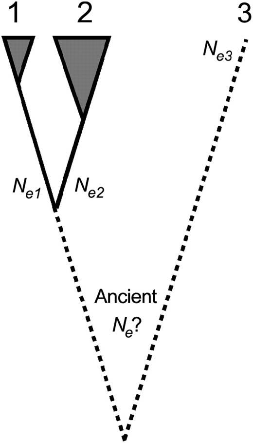
Basic three-species setting. We assume fixed values for all three effective population sizes Ne, despite uncertainty concerning the sizes of ancestral populations. The shaded areas indicate the availability of neutral and selected polymorphism data from the two more closely related species with different Ne. The dotted line to the third species indicates that our method for inferring the strength of purifying selection also applies to cases where only polymorphism data for two species exist.
To keep our model simple, we assume that there are at most two types of amino acid at a given nucleotide site: “preferred” and “unpreferred,” with at most one of the four possible nucleotides corresponding to the preferred state (our methods do not require us to identify preferred and unpreferred states from the data). At some sites, all possible variants may be effectively neutral, meaning in practice that variants are subject to a similar level of selection to silent mutations (Figure 2D). The fraction of such “neutral” nonsynonymous mutations is denoted by cn. We treat other sites as in Figure 2A, where nonsynonymous nucleotide site mutations can result in a change to a selectively deleterious amino acid (if the nucleotide in question codes for the preferred state), to a favorable amino acid (if the site is fixed for an unpreferred amino acid, and the mutation leads back to the preferred state), or else to a selectively neutral variant (if the site is fixed for an unpreferred amino acid, and the mutation causes a change to a different but selectively equivalent deleterious variant). Because some mutations at such sites are deleterious, we refer to these sites as undergoing purifying selection.
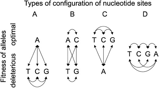
All possible fitness-relevant configurations for nondegenerate nucleotide sites. The four alternatives A, T, C, and G stand for any of the four possible nucleotides at a site. In configuration A, only one allele is optimal, whereas in D all alternatives are equally fit (i.e., they are mutually neutral). B and C allow for neutral mutations between equally optimal alternatives at sites that are capable of producing deleterious mutations. This study assumes that configurations B and C do not exist and estimates the frequency of configuration D from the data (cn). This will lead to upper limits on estimates of the frequencies of configurations A and D. As long as no further mutations occur at segregating sites (the infinite-sites assumption), all four possible alternatives can be collapsed to the specific case of two alleles described in the text.
The selection coefficient s for selectively deleterious variants refers to the reduction in fitness of heterozygotes; this may vary according to the site and amino acid in question. For convenience of calculation, dominance is assumed to be intermediate. As in standard models of codon usage bias (Li 1987; Bulmer 1991; McVean and Charlesworth 1999), if selection at these sites is sufficiently weak, unpreferred mutations can become fixed and then mutate back to the preferred state, contributing to a flux of amino acid substitutions as well as to polymorphism. This model is not completely general (see Figure 2, B and C), but should suffice as a guide to the basic processes involved, especially when selection is fairly strong in relation to drift.
Occasionally, a new adaptive mutation (distinct from a back mutation at a site fixed for a deleterious mutation) may arise at a nonsynonymous site, perhaps in response to a change in the environment. This is assumed to spread rapidly to fixation if it survives initial stochastic loss. The substitution rate per generation per site for mutations that fall into this category is denoted by cau, where u is the expected mutation rate per nucleotide site, and ca measures the substitution rate as a fraction of all mutations. ca is the product of the frequency of adaptive mutations and their fixation probability, integrated over all advantageous effects. We assume that ca ≪ 1, since favorable mutations are likely to be rare.
Strong purifying selection:
Arbitrary purifying selection:
The validity of the assumption that Nes > 1 for all nonneutral nonsynonymous mutations is, however, questionable. If this assumption is relaxed, the formulas for the equilibrium diversity at nonsynonymous sites become more complex, and the possibility of a contribution to KA from sites subject to purifying selection must also be considered, using a probability distribution ϕ(s) of selection coefficients for mutations subject to selection. We now consider this problem in detail.
As far as diversity is concerned, we note first that a nonsynonymous site that has become fixed for a mutant nucleotide coding for a deleterious amino acid can either mutate back to the original nucleotide or mutate to another nucleotide coding for a deleterious amino acid. If mutation rates among all four nucleotides were equal, the probability of back mutation to the original state would be
RESULTS
We now present the results of applying these methods to the diversity data on D. miranda and D. pseudoobscura described in materials and methods (D. miranda is designated as species 1 and D. pseudoobscura as species 2 in what follows). In view of such problems as the lack of overlap between the genes used in the two species, and the disparity in sample sizes between studies, the results based on these data should be regarded as merely provisional and illustrative of the methods.
Strong purifying selection:
We first present the results of applying the expectations for the case of strong purifying selection. Divergence values from D. affinis (species 3) were estimated for the 17 genes surveyed in D. miranda; the divergence values for these genes between D. affinis and D. pseudoobscura were almost identical (Bartolomé et al. 2005), so that only the D. miranda results were used here. Both weighted and unweighted estimates of mean diversities were obtained, as described in materials and methods; statistical uncertainty was assessed by bootstrapping across genes.
The results are displayed in Table 1. The main conclusion is that an estimate of
Summary of the data and estimates from the strong purifying selection model
Estimate | \(\mathrm{{\pi}}_{\mathrm{A}_{1}}\) | \(\mathrm{{\theta}}_{\mathrm{S}_{1}}\) | \(\mathrm{{\pi}}_{\mathrm{A}_{2}}\) | \(\mathrm{{\theta}}_{\mathrm{S}_{2}}\) | KA | KS | \(N_{\mathrm{e}_{1}}s_{\mathrm{h}}\) | cn | Pa |
|---|---|---|---|---|---|---|---|---|---|
| Weighted | 0.086 (0.041/0.136) | 0.502 (0.340/0.710) | 0.294 (0.196/0.400) | 2.86 (2.02/3.43) | 2.11 (1.28/2.80) | 23.0 (20.4/24.9) | 5.41 (2.84/ \({\infty}\) ) | 8.79 (3.91/16.5) | 3.99 (−123/57.5) |
| Unweighted | 0.088 (0.044/0.141) | 0.478 (0.342/0.626) | 0.206 (0.124/0.300) | 2.73 (2.31/3.14) | 2.48 (1.30/3.76) | 22.2 (19.9/24.8) | 3.58 (1.80/29.8) | 5.24 (0.923/10.3) | 52.9 (−28.9/93.3) |
All values except for
The estimated proportion of neutral sites was smaller with the unweighted estimates than with the weighted ones, but both suggested a value of a few percent. There was a very wide distribution of values of the proportion of fixations due to adaptive mutations in both cases, and a zero value could not be ruled out by the data, although the value estimated from the data exceeded 50% for the unweighted estimate.
Arbitrary purifying selection:
We now relax the assumption that πA is close to the deterministic prediction by applying the model behind Equations 5 to the same data. The assumptions of a gamma distribution of mutational effects, and that 0, 2.5, or 5% of all nonsynonymous mutations are neutral, yielded the parameters reported in Tables 2 and 3 for the weighted and unweighted data, respectively. With values of cn ≥ 7.5% we rarely, if ever, found parameters for a gamma distribution that fitted the data, and the fraction of bad fits for cn = 5% was 48.5% for 1000 bootstraps from the weighted data, whereas the mean of the unweighted data could not be fitted assuming cn ≥ 5%. With the gamma distribution, a significant fraction of mutations had such small selection coefficients that Nes < 1 or even 0.5. The results of McVean and Charlesworth (1999) suggest that, with Nes < 0.5, both diversities and substitution rates are nearly equivalent to those for neutral sites; in addition, the intensity of selection on synonymous mutations that change codon usage from preferred to unpreferred codons in D. miranda seems to be close to Nes = 0.5 (Bartolomé et al. 2005). It thus seems reasonable to use this value as the boundary for designating mutations as effectively neutral; the sum of cn and the fraction of effectively neutral mutations generated by the fitted gamma distribution is denoted by cne in Tables 2 and 3. For completeness, we also show results using Nes = 1 as the boundary.
Estimates of the distribution of mutational effects for variance-weighted data from D. miranda and D. pseudoobscura
cn (%) | α | loc | Species | Nes (am) | Nes (hm) | Nes (5%) | Nes (95%) | CV | cne (%) | \(P_{\mathrm{a}_{1}};P_{\mathrm{a}_{2}}\) (%) | \(P_{\mathrm{a}_{3}}\) (%) |
|---|---|---|---|---|---|---|---|---|---|---|---|
| 0 | 0.299 (0.0782/0.741) | 0.000266 (1.14 × 10⁻⁵/17,000) | mir | 255 (11.6/95,700) | 8.35 (3.49/17.9) | 1.31 (0.843/3.01) | 1,100 (36.9/558,000) | 1.67 (1.08/2.15) | 12.7 (7.91/17.0) | −42.8 (−125/14.7) | 0.902 (−83.5/60.3) |
| 263 (12.4/97,500) | 13.3 (4.82/31.7) | 2.22 (1.40/5.06) | 1,100 (37.8/560,000) | 1.64 (1.02/2.11) | 15.5 (11.0/20.2) | ||||||
| pso | 1,370 (55.3/521,000) | 14.4 (8.69/25.0) | 2.50 (1.55/5.47) | 6,220 (188/3,110,000) | 1.74 (1.14/2.22) | 7.57 (2.35/13.4) | 15.7 (−72.1/73.7) | ||||
| 1,400 (56.2/534,000) | 23.0 (11.8/43.8) | 3.72 (2.39/8.47) | 6,240 (188/3,200,000) | 1.72 (1.12/2.20) | 9.19 (3.65/14.7) | ||||||
| 2.5 | 0.448 (0.0996/1.32) | 7.67 × 10⁻⁵ (7.12 × 10⁻⁶/89.5) | mir | 70.6 (6.96/76,500) | 6.86 (3.19/17.2) | 1.21 (0.877/2.96) | 274 (18.4/463,000) | 1.39 (0.832/2.08) | 11.4 (5.73/16.6) | −31.1 (−117/27.9) | 7.93 (−78.7/57.7) |
| 73.1 (7.32/78,800) | 10.1 (3.99/29.9) | 1.93 (1.37/4.80) | 275 (18.8/476,000) | 1.36 (0.789/2.05) | 14.4 (9.04/19.3) | ||||||
| pso | 382 (35.4/392,000) | 14.7 (9.48/28.4) | 2.73 (1.77/7.31) | 1,550 (97.2/2,450,000) | 1.45 (0.865/2.13) | 6.58 (2.87/13.4) | 16.4 (−70.0/59.1) | ||||
| 388 (35.4/401,000) | 21.5 (12.2/45.5) | 3.96 (2.59/9.77) | 1,550 (97.2/2,490,000) | 1.43 (0.857/2.12) | 7.95 (3.30/14.6) | ||||||
| 5 | 0.831 (0.228/1.75) | 2.33 × 10⁻⁵ (6.84 × 10⁻⁶/0.0179) | mir | 20.4 (6.53/11,400) | 5.42 (3.39/18.9) | 1.21 (0.931/3.53) | 63.6 (15.8/55,700) | 1.05 (0.737/1.95) | 9.27 (6.40/16.1) | −11.2 (−113/22.6) | 15.2 (−78.3/38.3) |
| 21.1 (6.72/11,600) | 7.07 (4.08/31.5) | 1.76 (1.42/5.40) | 63.7 (16.2/55,800) | 1.02 (0.702/1.93) | 12.2 (8.41/19.0) | ||||||
| pso | 112 (31.7/80,400) | 17.4 (10.5/35.2) | 4.28 (2.13/10.9) | 362 (80.1/413,000) | 1.09 (0.753/1.98) | 6.01 (5.08/12.1) | 14.4 (−73.1/35.6) | ||||
| 113 (32.0/81,200) | 21.5 (12.5/53.0) | 4.73 (2.93/13.1) | 362 (80.2/415,000) | 1.08 (0.746/1.97) | 6.72 (5.22/13.7) |
The Nes values reported here describe the distribution of deleterious mutational effects for all effectively nonneutral and nonlethal sites, where (am) denotes the arithmetic mean and (hm) the harmonic mean; (5%) and (95%) represent the lower and upper fifth percentiles of this truncated distribution; mir and pso refer to D. miranda and D. pseudoobscura, respectively; cn is the fraction of completely neutral mutations assumed in the calculations; cne is the fraction of effectively neutral mutations; CV denotes the coefficient of variation of Nes values of the truncated distribution;
Estimates of the distribution of mutational effects for unweighted data from D. miranda and D. pseudoobscura
cn (%) | α | loc | Species | Nes (am) | Nes (hm) | Nes (5%) | Nes (95%) | CV | cne (%) | \(P_{\mathrm{a}_{1}};P_{\mathrm{a}_{2}}\) (%) | \(P_{\mathrm{a}_{3}}\) (%) |
|---|---|---|---|---|---|---|---|---|---|---|---|
| 0 | 0.562 (0.172/1.62) | 2.75 × 10⁻⁵ (4.25 × 10⁻⁶/0.0732) | mir | 24.3 (3.89/62,700) | 4.76 (2.20/16.4) | 0.978 (0.730/2.67) | 87.6 (9.76/347,000) | 1.23 (0.735/1.96) | 9.93 (4.43/14.4) | 4.03 (−61.3/49.9) | 51.5 (−12.7/91.1) |
| 25.6 (4.21/63,700) | 6.77 (2.83/29.1) | 1.56 (1.19/4.52) | 88.5 (9.84/348,000) | 1.18 (0.666/1.93) | 14.2 (8.73/20.9) | ||||||
| pso | 130 (19.7/320,000) | 11.6 (7.72/24.3) | 2.22 (1.65/5.49) | 471 (51.4/1,760,000) | 1.30 (0.784/2.02) | 3.71 (0.332/8.86) | 64.2 (−2.18/96.5) | ||||
| 133 (19.8/324,000) | 16.1 (9.39/41.3) | 3.02 (2.28/7.80) | 472 (51.5/1,770,000) | 1.28 (0.780/2.00) | 5.33 (0.965/9.99) | ||||||
| 2.5 | 1.05 (0.267/2.48) | 1.20 × 10⁻⁵ (4.92 × 10⁻⁶/0.00238) | mir | 10.0 (3.91/2,050) | 3.87 (2.41/15.6) | 0.987 (0.786/2.63) | 29.8 (8.97/9,060) | 0.930 (0.624/1.80) | 7.13 (3.53/13.4) | 25.4 (−48.1/57.8) | 58.4 (−11.7/73.6) |
| 10.5 (4.11/2,070) | 4.95 (2.94/24.8) | 1.46 (1.23/4.07) | 30.0 (9.06/9,110) | 0.887 (0.591/1.78) | 11.3 (5.76/18.3) | ||||||
| pso | 55.2 (21.9/11,300) | 14.0 (8.81/29.2) | 3.53 (2.07/8.57) | 161 (50.1/50,700) | 0.968 (0.634/1.84) | 3.25 (2.52/8.07) | 61.2 (−5.50/73.7) | ||||
| 55.6 (22.2/11,300) | 16.3 (10.7/43.9) | 4.09 (2.71/9.88) | 161 (50.8/50,700) | 0.960 (0.633/1.83) | 3.95 (2.58/9.58) |
See Table 2 for explanation.
Despite the time-consuming nature of the multiple integrations involved in implementing this model, we attempted 1000 bootstrap replications to assess the reliability of our parameter estimates. Out of these bootstrap computations for the weighted or unweighted data in Table 2 or 3, only 80.3 and 90.1%, respectively, could be fitted assuming cn = 0%; 75.6 and 65.6% could be fitted assuming cn = 2.5%. Technically, our estimates of the distributions of mutational effects involve only the shape and the location parameter for the gamma distribution of s, together with values for
As reviewed in more detail in the discussion, the bulk of the nonneutral mutations segregating in the population come from the more weakly selected tail of the distribution (Sunyaev et al. 2001). The arithmetic mean of the distribution of selection coefficients among these polymorphic variants is much closer to the harmonic than to the arithmetic mean of the distribution for new mutations, and so the harmonic means in Tables 2 and 3 are more relevant than the arithmetic means to the properties of mutations found in populations. It is notable from Tables 2 and 3 that the means for D. pseudoobscura were smaller than might be expected from the ratio of effective population sizes and the corresponding means for D. miranda; this reflects the lower fraction of mutations that fall into the effectively neutral class when the effective population size is larger, reducing the average selection coefficients for mutations in the other class.
Given an ancestral Ne-value, we can also predict the substitution rate for mutations under purifying selection. This can be compared with the observed rate to estimate the proportion of adaptive substitutions, using Equation 4. We report three alternative values:
The main result of Tables 2 and 3 is solid support for the conclusion that ∼90% or more of all amino acid mutations have significantly deleterious effects. It is also remarkable that the estimates of the biologically important harmonic mean selection coefficient are close to those using the strong selection assumption, taking into account the statistical noise and the uncertainty regarding cn for the arbitrary purifying selection model. Similar conclusions can be drawn for comparisons between cne in the arbitrary purifying selection model and cn in the strong selection model. Comparing the weighted and unweighted estimates shows that the weighting procedure influences the estimates, but the noise in the data is larger than the noise from uncertainty about the best weighting procedure. While our definitions of effective neutrality (Nes < 0.5 or < 1) have little influence on the arithmetic mean and the upper fifth percentile of the distribution of mutational effects, their influence on the harmonic mean and the lower fifth percentile is greater. In no case, however, did the ∼1–3% of mutations that fall in the range 0.5 < Nes < 1 change our conclusions regarding the prevalence of deleterious mutations.
To visualize the gamma distributions of mutational effects estimated from the weighted data, we plotted our best-fitting estimates with assumed values of cn = 0, 2.5, and 5% (Figure 3). This involved estimating effective population size from Equation 1a, using the “standard” mutation rate of 1.5 × 10⁻⁹. The distributions for the two smaller values of cn peaked at selection coefficients ∼10−4, fairly close to the arithmetic means obtained from Table 2 for mutations that are not effectively neutral, whereas the harmonic mean was about one-tenth of this.
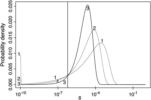
Gamma distributions of mutational effects estimated from the variance-weighted data, assuming cn = 0, 2.5, and 5% (curves 1, 2, and 3, respectively). The spike below s = 10−10 corresponds to the integral of the distribution from 0 up to this value. The vertical line corresponds to Nes = 0.5 for D. miranda. The computations assume u = 1.5 × 10⁻⁹ and κ = 2. Note the use of a log scale for the selection coefficients.
DISCUSSION
Robustness of the strong purifying selection model:
We found quite good agreement between the results of the strong purifying selection model and the model with a gamma distribution of selection coefficients for the estimates of the harmonic mean of the selection coefficient. This suggests that estimates of the magnitude of this important parameter are robust to the assumptions used, providing that a sizeable fraction of nonsynonymous polymorphisms is nonneutral. Some approximations that relax the assumptions of the strong purifying selection model, but that do not depend on the details of the distribution, are explored in the appendix. These provide very general methods for estimating Nesh and again suggest that the magnitudes of the estimates of the main parameters of interest are fairly robust to details of the assumptions.
This result is remarkably robust, since we do not need to know Ne, u, sh, or dominance coefficients. However, caution is necessary if Equation 8b gives values near 1, since this suggests that drift is probably too strong to be neglected. In this case, the true strength of selection for the deleterious mutations will be larger than predicted by this approach. The values estimated from this method are Nesh ≈ 2.9 and 4.9 for D. miranda and D. pseudoobscura, as estimated for the respective weighted data. These values are little more than a third of the respective values estimated from the most precise methods and lie outside the confidence intervals for the latter. This very simple formula is therefore too crude for precise estimates, but seems to work reasonably well as a rough first estimate for the lower bound of Nesh. It can be applied only when there is evidence that a substantial proportion of segregating nonsynonymous variants experience purifying selection, as in the present case (Bartolomé et al. 2005).
One caveat should be noted concerning the estimates of Ne for D. pseudoobscura that we have been using. This assumes that silent sites are effectively neutral, which we have taken to mean that Nes is of the order of ≤0.5 McVean and Charlesworth (1999). While D. miranda synonymous sites seem to satisfy this condition (Bartolomé et al. 2005), this condition clearly cannot apply to D. pseudoobscura, given that mean silent diversity is four to five times higher than that in D. miranda, unless selection on synonymous sites is much weaker in D. pseudoobscura. Akashi and Schaeffer (1997) estimated Nes against unpreferred codons to be 4.6 (95% confidence interval 2.4–12.1) for Adh plus Adhr in D. pseudoobscura, (although selection for preferred codons was negligible); this result may be in part confounded by the effects of population expansion. If Nes for synonymous sites in D. pseudoobscura is indeed higher than that in D. miranda, then mean silent site diversity (which includes a large contribution from synonymous sites) will yield an underestimate of 4Neu for this species. Accordingly, Nes for nonsynonymous sites will be underestimated and the proportion of effectively neutral nonsynonymous mutations overestimated, since the ratio of nonsynonymous diversity relative to effectively neutral diversity will be overestimated for this species.
Sensitivity to mutation rates, mutational bias, and recombination rates:
Estimates derived from the arbitrary purifying selection model are surprisingly insensitive to plausible changes in mutational bias and mutation rate. Drake et al. (1998, p. 1673) estimated from laboratory experiments that 8.5 × 10⁻⁹ mutations per base per generation happen in D. melanogaster. Powell (1997, p.369–371) reported rates between 0.67 × 10⁻⁹ and 3.3 × 10⁻⁹, estimated from divergence between the D. melanogaster and D. obscura groups, assuming that divergence happened 30 MYR ago and that each year represents ∼10 generations. McVean and Vieira (2001) estimated a rate of 1.5 × 10⁻⁹ (95% C.I. = 1.0 × 10⁻⁹–2.5 × 10⁻⁹), assuming 2–4 MYR divergence between D. melanogaster and D. simulans. Others (Andolfatto and Przeworski 2000; Przeworski et al. 2001) found rates of between 0.6 × 10⁻⁹ and 4.75 × 10⁻⁹. Thus 0.5 × 10⁻⁹ and 8 × 10⁻⁹ appear to be reasonable choices for the most extreme lower and upper credible limits for mutation rates in Drosophila. As can be seen in Table 4, when cn = 2.5%, a mutational bias of κ = 1 leads to the largest differences from our other estimates, while large changes in mutation rate seem to have only minor effects. Other assumed values of cn yield the same conclusion, although the resulting estimates differ because of the strong influence of cn (see Tables 2 and 3).
The influence of mutation rate u and mutational bias κ on estimates of cne,
u = 0.5 × 10⁻⁹ | u = 2 × 10⁻⁹ | u = 8 × 10⁻⁹ | |
|---|---|---|---|
| κ = 1 | 10.8% | 10.9% | 11.0% |
| 6.51 | 6.59 | 6.67 | |
| 0.486 | 0.477 | 0.469 | |
| κ = 2 | 11.3% | 11.4% | 11.5% |
| 6.88 | 6.95 | 7.03 | |
| 0.453 | 0.447 | 0.441 | |
| κ = 3 | 11.4% | 11.5% | 11.6% |
| 6.95 | 7.02 | 7.10 | |
| 0.452 | 0.446 | 0.440 |
The top value in each row gives cne (in percent). The middle value gives
Three genes in our D. pseudoobscura data set (Amy1, eve, and exu1) are located on Muller's C, a genomic region that is segregating for paracentric inversions (Dobzhansky and Powell 1975) and therefore has a highly reduced recombination rate. These three genes violate the assumption of independence of sites much more than the other genes. We ran 500 bootstraps for a variance weighted data set without these genes under the assumption of cn = 0%. Results indicate that the inclusion of these genes does not strongly affect our parameter estimates, as the confidence intervals of our estimates for the reduced data set mostly overlap our estimates for the full data set (data not shown).
The reliability of estimates of the proportion of adaptive mutations:
As can be seen from Figure 4, there is a large influence of the value of the (unknown) ancestral Ne on the estimate of the proportion of adaptive mutations. As expected from the fact that more slightly deleterious mutations can be fixed in smaller populations, fewer adaptive mutations are inferred with smaller ancestral Ne-values (Eyre-Walker 2002). Again, the mutation rate and mutational bias do not greatly affect the estimates. The combination of Figure 4 with the wide confidence intervals for Pa from Tables 1–3 raises the question of whether this approach can determine the presumably small fraction of adaptive mutations with any precision. Larger data sets and the use of the same sets of genes in the two species being compared may help to narrow the error bounds on the estimates.
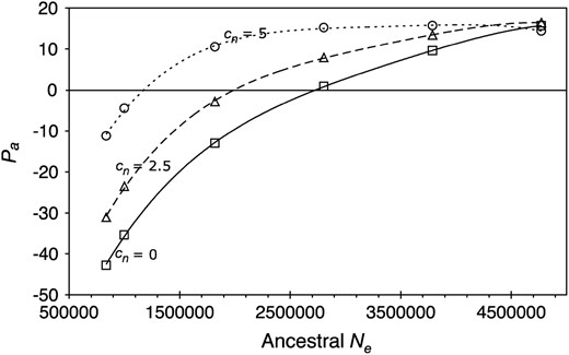
Dependence of estimates of the proportion of adaptive mutations (Pa) on ancestral Ne. All values were computed from the variance-weighted data and assume u = 1.5 × 10⁻⁹; κ = 2; and cn = 0, 2.5, and 5% for the solid, dashed, and dotted curves, respectively. The smallest and largest values of Ne correspond to the estimates of current Ne for D. miranda and D. pseudoobscura, respectively.
However, potential difficulties still remain. One is the assumption of free recombination among variants. Linkage increases the rate of fixation of deleterious mutations while decreasing that for advantageous mutations (Birky and Walsh 1988); close linkage can have important effects even with weak selection (McVean and Charlesworth 2000; Kim 2004). But this assumption seems reasonable for D. pseudoobscura and its relatives, with their high rates of recombination and lack of linkage disequilibrium within genes (Dobzhansky and Powell 1975; Schaeffer and Miller 1993; Yi et al. 2003). In addition, departures from equilibrium due to demographic effects may introduce errors into the estimates. As discussed in materials and methods, our choice of θW instead of π as a synonymous diversity estimator is intended to minimize the effects of the population expansion that seems to have occurred in D. pseudoobscura (Machado et al. 2002; Schaeffer 2002). However, we cannot exclude population bottlenecks in the distant past that could have led to a higher contribution of deleterious mutations to KA/KS relative to πA/πS and thus have elevated the estimate of the proportion of adaptive substitutions (Eyre-Walker 2002), a problem common to all methods used to date.
The reliability of estimates of parameters of the distribution of mutational effects:
Methods of estimating selection parameters for deleterious mutations that assume a distribution of selection coefficients make inferences about the distribution for new mutations prior to the action of selection, on the basis of the properties of mutations that are segregating in populations; these have been exposed to a long history of selection. The arithmetic mean s for segregating mutations is obtained by summing the products of the selection coefficient at each site i by the corresponding frequency of heterozygotes
Tables 2 and 3 show that the mean of the prior gamma distribution can be much larger than the harmonic mean for mutations above the effective neutrality threshold, indicating that much of the probability mass of the gamma distribution is far from the s-values representative of segregating mutations. This raises a serious issue concerning the meaning of inferences concerning the parameters of the gamma distribution; these are based on the properties of mutations that have little relation to the bulk of the mutations in the prior distribution.
With this caveat in mind, one of the strongest results from our arbitrary purifying selection model is not the exact set of parameter values themselves, but rather the exclusion of the large number of parameter combinations that are not compatible with the data. Our difficulties fitting distributions of mutational effects for cn ≥ 5%, for example, probably suggest that <5% of all nonsynonymous mutations stem from a small set of mutational effects distinct from the continuous distribution, which behave as neutral. Similarly, Tables 2 and 3 allow us to restrict the credible range for the shape parameter of a gamma distribution to shapes >0.1 and usually <1, where 1 is equivalent to an exponential distribution; not many credible estimates have less leptokurtic shapes. This agrees with results for mitochondrial genes, based on a different approach (Piganeau and Eyre-Walker 2003).
If our estimates of the arithmetic and harmonic means of the distribution of s are even approximately correct (of the order of 10−4 and 10−5, respectively; see results), they imply that most deleterious nucleotide substitutions affecting protein sequences in our two species are subject to very weak selection. This seems inconsistent with the classical estimates of harmonic mean heterozygous selection coefficients of the order of 1% in D. melanogaster, obtained by comparing inbreeding loads for viability with the mutational decline in mean viability, as well as with estimates of mean homozygous selection coefficients of the order of ≥10% obtained from mutation-accumulation experiments (Crow 1993; Charlesworth and Hughes 2000; Charlesworth et al. 2004). The former are, however, biased upward by being weighted by the selection coefficients themselves, and the latter are known to be biased upward when there is a wide distribution of homozygous selection coefficients (Crow 1993). In addition, it is likely that insertional mutations that effectively knock out gene function, like those caused by transposable elements, contribute substantially to these estimates (Keightley and Eyre-Walker 1999; Charlesworth et al. 2004). In contrast, the estimates of heterozygous selection coefficients of the order of 10−3, obtained from a population screen for null alleles at enzyme loci in D. melanogaster by Langley et al. (1981), are consistent with our estimates, assuming that they represent the effects of loss of function at nonvital loci. As pointed out to us by Allen Orr (A. Orr, personal communication), it is difficult to reconcile the results of the null allele screen with the classical estimates of average selection coefficients for deleterious mutations.
Perspectives for the future:
An obvious way to narrow the confidence intervals is the compilation of data sets with more genes. This does not, however, solve the conceptual problem that more degrees of freedom are needed to estimate more parameters. One way of obtaining additional degrees of freedom is to use shared polymorphisms to obtain an estimate of ancestral Ne (Wakeley and Hey 1997). Since ∼3% of the polymorphisms in D. miranda and D. pseudoobscura seem to be shared by both species (Charlesworth et al. 2005), this is in principle possible. In the present study, we have ignored this approach, due to limited statistical power (only three suitable loci have been surveyed in both species). Another possibility for estimating additional parameters is to use sets of three species where significant differences can be observed in KA/KS as well as in πA/πS. This might eventually allow simultaneous estimation of Pa and cn as well as of the shape and location parameters of the distribution of mutational effects. We also deliberately did not classify amino acid changes according to conservative, radical, etc., to keep the model simple. There is no reason why this could not be done with larger data sets, by dividing observations of πA into several classes according to an a priori classification of their effects on protein function (Sunyaev et al. 2001; Williamson et al. 2005).
APPENDIX: EXTENDING THE STRONG PURIFYING SELECTION MODEL
A similar relation can be written for species 2 (the species with larger Ne), retaining the same values of s′ and ψ(s). The only change is that
This approach provides a conservative method for improving on the assumption of strong purifying selection, without having to make specific assumptions about the distribution of mutational effects. Application of this method to the weighted data on D. miranda and D. pseudoobscura, assuming γ1′ = 2 and a mutational bias of 2, gave estimates of cne of 4.5% (−1.6%/11.6%),
Use of Equation 3a of the text provides an upper-bound estimate of cne, since it assumes that all deleterious mutations outside the effectively neutral range have s-values sufficiently large that the deterministic expression in Equation 2a is valid, ignoring mutations with very small s-values. 1/sh in Equation 2a must therefore be smaller than the values allowing for a wider distribution of s-values, and so cn must be larger. The true value of cne is thus likely to lie between the estimates from Equations 3a and A2.
Given the uncertainties involved, the degree of concordance between the estimates of
An even more conservative lower bound on
This estimate can be applied to any suitable data set on coding sequence polymorphisms, as long as a credible assumption about cne can be made. For example, Sunyaev et al. (2000) reported an estimate of 0.33 for the ratio of diversity at nondegenerate coding sites to fourfold degenerate sites, in a large-scale survey of EST-based human SNPs. With κ = 2 and I = 0.787, we get Nesh ≥ 1.18 for cne = 0. With an effective population size for humans of ∼10,000, this suggests a harmonic mean selection coefficient for nonneutral amino acid variants of at least 1.18 × 10⁻⁴. Other studies have suggested that ∼20% of amino acid variants in humans are effectively neutral (Fay et al. 2001; Sunyaev et al. 2001); if this value of cne is used in expression (A3), the estimate of Nesh for nonneutral variants becomes 2.42.
Footnotes
Present address: Unidade de Xenética Evolutiva, Instituto de Medicina Legal, Facultade de Medicina, Universidade de Santiago de Compostela, 15782 Santiago de Compostela, Spain.
Footnotes
Communicating editor: S. W. Schaeffer
Acknowledgement
We thank Deborah Charlesworth, Stephen Schaeffer, and two anonymous reviewers for comments on the manuscript. This work was supported by grants from the Biotechnology and Biological Sciences Research Council, the Leverhulme Trust, and the Royal Society.
References
Akashi, H.,
Akashi, H., and S. W. Schaeffer,
Andolfatto, P., and M. Przeworski,
Bartolomé, C., X. Maside, S. Yi, A. L. Grant and B. Charlesworth,
Bierne, N., and A. Eyre-Walker,
Birky, Jr., C. W., and J. B. Walsh,
Bulmer, M.,
Bustamante, C. D., R. Nielsen, S. A. Sawyer, K. M. Olsen, M. D. Purugganan et al.,
Bustamante, C. D., R. Nielsen and D. L. Hartl,
Bustamante, C. D., A. Fledel-Alon, S. Williamson, R. Nielsen, M. T. Hubisz et al.,
Charlesworth, B., and K. A. Hughes,
Charlesworth, B., H. Borthwick, C. Bartolome and P. Pignatelli,
Charlesworth, B., C. Bartolomé and V. Noël,
Crow, J. F.,
Dobzhansky, T., and J. R. Powell,
Drake, J. W., B. Charlesworth, D. Charlesworth and J. F. Crow,
Eyre-Walker, A.,
Fay, J. C., G. J. Wyckoff and C. I. Wu,
Haldane, J. B. S.,
Haldane, J. B. S.,
Hartl, D. L., E. N. Moriyama and S. A. Sawyer,
Ihaka, R., and R. Gentleman,
Keightley, P. D., and A. Eyre-Walker,
Kim, Y.,
Kimura, M.,
Kimura, M.,
Kimura, M.,
Kimura, M., and T. Ohta,
Kimura, M., and T. Ohta,
Langley, C. H., R. A. Voelker, A. J. Brown, S. Ohnishi, B. Dickson et al.,
Li, W. H.,
Machado, C. A., R. M. Kliman, J. A. Markert and J. Hey,
McDonald, J. H., and M. Kreitman,
McVean, G. A. T., and B. Charlesworth,
McVean, G. A. T., and B. Charlesworth,
McVean, G. A. T., and J. Vieira,
Nachman, M. W.,
Nelder, J. A., and R. Mead,
Orr, H. A., and Y. Kim,
Piganeau, G., and A. Eyre-Walker,
Powell, J. R.,
Przeworski, M., J. D. Wall and P. Andolfatto,
Rand, D. M., and L. M. Kann,
Rand, D. M., and L. M. Kann,
Rozas, J., J. C. Sanchez-DelBarrio, X. Messeguer and R. Rozas,
Sawyer, S. A.,
Sawyer, S. A., and D. L. Hartl,
Sawyer, S. A., D. E. Dykhuizen and D. L. Hartl,
Sawyer, S. A., R. J. Kulathinal, C. D. Bustamante and D. L. Hartl,
Schaeffer, S. W.,
Schaeffer, S. W., and E. L. Miller,
Sunyaev, S., V. Ramensky, I. Koch, W. Lathe, III, A. S. Kondrashov et al.,
Sunyaev, S. R., W. C. Lathe, III, V. E. Ramensky and P. Bork,
Tajima, F.,
Wakeley, J., and J. Hey,
Watterson, G. A.,
Weinreich, D. M., and D. M. Rand,
Williamson, S., A. Fledel-Alon and C. D. Bustamante,
Williamson, S. H., R. Hernandez, A. Fledel-Alon, L. Zhu, R. Nielsen et al.,
Wright, A., B. Charlesworth, I. Rudan, A. Carothers and H. Campbell,
Yi, S., D. Bachtrog and B. Charlesworth,
