
Abstract
Ultrasonic analysis was used to predict the state of charge and state of health of lithium-ion pouch cells that have been cycled for several hundred cycles. The repeatable ultrasonic trends are reduced to two key metrics: time of flight shift and total signal amplitude, which are then used with voltage data in a supervised machine learning technique to build a model for state of charge (SOC) prediction. Using this model, cell SOC is predicted to ∼1% accuracy for both lithium cobalt oxide and lithium iron phosphate cells. Elastic wave propagation theory is used to explain that the changes in ultrasonic signal are related to changes in the material properties of the active materials (i.e., elastic modulus and density) during cycling. Finally, we show the machine learning model can accurately predict cell state of health with an error ∼1%. This is accomplished by extending the data inputs into the model to include full ultrasonic waveforms at top of charge.
Export citation and abstract BibTeX RIS

This is an open access article distributed under the terms of the Creative Commons Attribution Non-Commercial No Derivatives 4.0 License (CC BY-NC-ND, http://creativecommons.org/licenses/by-nc-nd/4.0/), which permits non-commercial reuse, distribution, and reproduction in any medium, provided the original work is not changed in any way and is properly cited. For permission for commercial reuse, please email: oa@electrochem.org.
A key component of an electric vehicle is the battery management system (BMS), which is responsible for controlling the operating conditions on a given battery cell (or stack of cells) in order to optimize the performance and lifetime of the full battery system. The most effective battery management systems must be able to track battery state of charge (SOC), state of health (SOH) and cell failure, including early prediction of catastrophic failure. Despite the importance of this task, being able to reliably determine SOC, SOH and failure at low cost still presents a significant challenge. A range of methods exist at present, however the simplest methods can prove inaccurate, and more complex methods are not suitable for low-cost, in-operando SOC determination.1–3
For instance, in its most common implementation, SOC prediction consists of voltage monitoring (direct measurement) combined with coulomb-counting (book-keeping).1 This can present challenges for a variety of reasons. First, for voltage measurements, the flatness of voltage readings over the majority of battery capacity, especially for lithium iron phosphate (LFP) cells, presents difficulties.4 Furthermore, voltage fade, changing cell impedances, and varying discharge rates impact measured voltage, obscuring true SOC. Second, coulomb counting is also an inexact science, as discharge rate, environmental factors such as temperature, and cell degradation can all impact the actual capacity for any given discharge. This can lead to a cycle of abuse, whereby discharge conditions lead to an incorrect estimate of SOC, and therefore the cell becomes inadvertently over-discharged. This causes damage to the cell, which leads to further inaccuracy in the SOC prediction, resulting in continued over-discharging and cell damage. Effectively, a battery "death-spiral" ensues.
One method to further increase the accuracy of battery management systems is to introduce a technique that can directly measure the physical state of the battery to enhance the determination of SOC, SOH, and cell failure, especially when applied in conjunction with existing electrically-based methodologies. Recently, ultrasonic techniques have been applied to batteries to understand cell behavior.5–8 Hsieh et al.5 first introduced the concept, applying 2.25 MHz ultrasonic pulses in transmission and pulse-echo modes to lithium-ion pouch cells, and both lithium-ion and alkaline cylindrical cells. Ultrasonic waveforms were measured over a time of flight range of ≤ 20 μs, and measurements were taken across all states of charge during cycling. They concluded there was a definite link between the SOC and ultrasonic signals from the cell, which they suggested was a result of material property changes within a cell during electrochemical cycling. Extending their hypothesis, they proposed that SOC and SOH could be determined using this method, but they did not investigate the matter further.
More recently, Chou et al.8 applied this technique to predicting state of charge in a vanadium redox flow battery (VRFB) by exploiting density variations in the vanadium electrolyte during operation. The advantages of a fixed flow channel and transducer geometry, and isotropic/homogeneous liquid state is that it allows for relatively straight-forward SOC determination. This illustrated the broad applicability and effectiveness of ultrasonic methods for determining battery properties.
Finally, Gold et al.7 applied this technique to a single lithium-ion pouch cell and demonstrated a proof of concept for SOC determination over one cycle, but they stopped short of showing how this technique can be incorporated into a practical BMS for SOC determination over many cycles. They applied ultrasonic pulses at a frequency which is an order of magnitude lower than the one used by Hsieh et al. (200 kHz vs. 2.25 MHz). The use of a lower frequency made it possible to analyze the arrival time of the slow, compressional wave, which would be difficult to resolve at higher frequencies due to increased attenuation of the ultrasonic wave. They proposed a link between the state of charge and changes in arrival time of the slow, compressional wave using poroelastic theory applied to the graphite electrode.
This work seeks to expand upon recent efforts by demonstrating the use of ultrasonic methods for practical prediction of SOC and SOH. In this manuscript, we study electrochemical-mechanical relationships using higher frequency ultrasonic methods similar to Hsieh et al. (∼2.25 MHz). High frequency transducers are used for practical reasons because they offer an opportunity for smaller packaging, such as through the use of MEMS piezoelectric transducers, since the active element thickness is inversely proportional to ultrasonic wavelength.9
In this work, the changes in state of charge and state of health are linked to variations in the first arrival time of the high frequency ultrasonic wave. According to elastic wave propagation theory, the wave propagation speed depends upon the bulk modulus, shear modulus, and density within a material.10 We claim that electrochemical changes within the host intercalation materials results in their mechanical properties changing as the battery cycles. This manifests itself as a change in the properties of the electrode materials as a whole, which leads to shifts in the transmitted ultrasonic signal at MHz frequencies.
Despite cell variability2,3,11 and measurement noise, we demonstrate that practical determination of state of charge is possible, beyond a proof of concept. This technique relies on an ultrasonic library of similar cells being generated, with the data then fed into a machine learning algorithm. The output can then be used with independent cell acoustic data to accurately determine state of charge and state of health, despite the battery performance and cycle history varying on a cell to cell basis.
Methods
This section provides an overview of the fundamentals of acoustic time of flight analysis of a battery. To conduct an acoustic experiment, the pulser-transducer sends an enveloped sinusoidal compressional pulse through the lithium-ion cell, and the signal is received by a transducer on the opposing side of the cell (Figure 1). The wave propagates through the cell, which consists of many thin material layers with thicknesses in the tens of microns (i.e., anodes, cathodes, separators, and current collectors). The propagation velocity of the compressional wave in each layer depends on the material properties of the media through which the wave is traveling. For an isotropic elastic material, this wave velocity is:
![Equation ([1])](https://content.cld.iop.org/journals/1945-7111/164/12/A2746/revision1/d0001.gif)
where K and G are the material bulk and shear moduli respectively, and ρ is the material density. At material interfaces the waves will be in part reflected and in part transmitted. Any waves striking at an angle to an interface may undergo mode conversion and partially propagate as shear waves.10 In this experiment we use compressional wave transducers, and measure with one pair of aligned transducers, so we only expect to measure contributions from compressional waves.
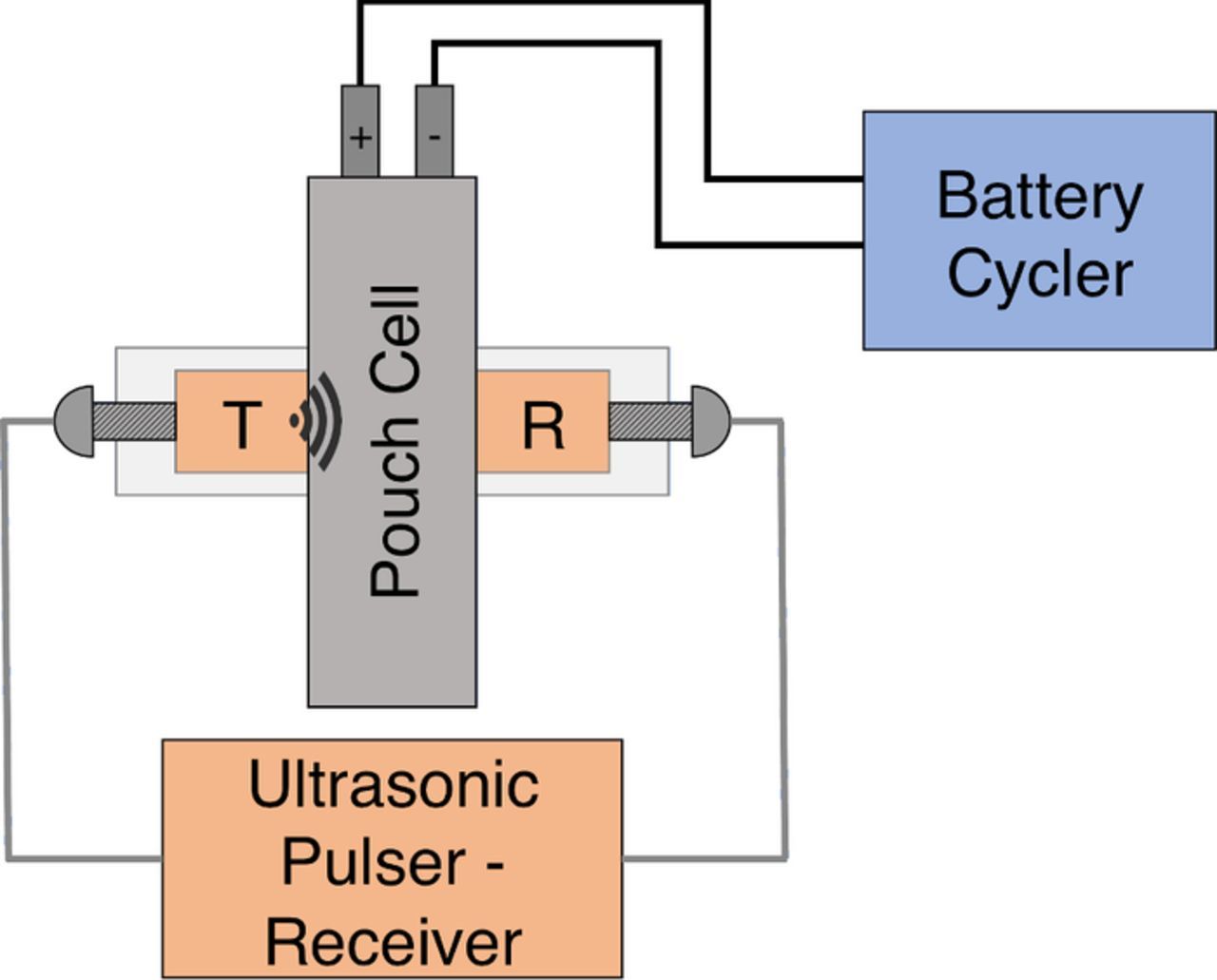
Figure 1. The battery cycler and ultrasonic pulser-receiver setup. Batteries are concurrently cycled and ultrasonically imaged.
Wave behavior through a finely layered structure such as a lithium ion battery differs from that through a non-finely layered structure. For waves with wavelength λ, much larger than the layer thickness, l, (ie λ ≫ l), the propagation speed through the complete thickness can be significantly different than the wave propagation speed that would be expected for waves propagating through a simple aggregation of the layers at their average wave-speed. Differences of the order of 20% or more in wavespeed are not uncommon.12 This is known as Backus averaging. In this case, the first wave arrival is slowed compared with the expected arrival time by this effect. In this paper we only explore the changes in wave propagation times, as opposed to absolute wave arrival times, for different electrochemical states, and therefore ignore this effect. It should be noted that this would be expected to slightly vary the time of flight results, as overall propagation speed is impacted. If first arrival times were to be determined, these effects would need to be included.
Using literature values for the mechanical properties for the cathode and anode active materials, binder and conductive additives, we can estimate a series of values for the bulk and shear moduli of the composite electrodes at varying states of charge. These can then be used to estimate changes in propagation time through the cell.
From the elastic modulus and Poisson's ratio, a material's bulk and shear moduli can be estimated according to Equations 2 and 3.13 We assume that the materials are isotropic or aggregates of randomly oriented polycrystals which are effectively isotropic.14
![Equation ([2])](https://content.cld.iop.org/journals/1945-7111/164/12/A2746/revision1/d0002.gif)
![Equation ([3])](https://content.cld.iop.org/journals/1945-7111/164/12/A2746/revision1/d0003.gif)
K and G are the bulk and shear moduli respectively, and ν is Poisson's ratio.
The positive and negative electrodes are porous composites of active material, binder, and conductive additives filled with electrolyte. It is possible to estimate effective electrode stiffness using Hashin-Shtrikman (HS) bounds,15,16 which provide a tighter bound on properties than the Voigt and Reuss bounds for composite materials. The Hashin-Shtrikman bounds represent the composite as being made up of an aggregation of spheres and shells of the constituent materials.
Equations 4–7 describe the maximum and minimum bounds for the bulk and shear moduli of the composite electrodes, based on the properties of the constituent components. In order to estimate a single value of each of the moduli for theoretical calculations, we take an average of the maximum and minimum HS bounds for bulk and shear moduli. At each cell SOC, bulk and shear moduli are calculated for each composite electrode. The moduli vary with SOC as the properties of the constituent materials vary. Equation 1 can then be used to determine the primary wave speed for each SOC. The change in the time of wave propagation with SOC can then be calculated.
![Equation ([4])](https://content.cld.iop.org/journals/1945-7111/164/12/A2746/revision1/d0004.gif)
![Equation ([5])](https://content.cld.iop.org/journals/1945-7111/164/12/A2746/revision1/d0005.gif)
![Equation ([6])](https://content.cld.iop.org/journals/1945-7111/164/12/A2746/revision1/d0006.gif)
![Equation ([7])](https://content.cld.iop.org/journals/1945-7111/164/12/A2746/revision1/d0007.gif)
Equations 8–10 are the functions lambda, gamma and zeta referenced in Equations 4–7 above. In Equations 8 and 9, the terms K(r) and G(r) represent the spatially varying moduli of the constituent material through the electrode. The variable z is given by the calling equation. In the case of Equations 6–7 this is also a function of zeta, Equation 10. The expectation value calculation in Equations 8 and 9 is a volume fraction weighted average.
![Equation ([8])](https://content.cld.iop.org/journals/1945-7111/164/12/A2746/revision1/d0008.gif)
![Equation ([9])](https://content.cld.iop.org/journals/1945-7111/164/12/A2746/revision1/d0009.gif)
![Equation ([10])](https://content.cld.iop.org/journals/1945-7111/164/12/A2746/revision1/d0010.gif)
Physically, the maximum and minimum analytical values of the moduli depend on which of the constituent materials form the sphere or shells of the composite material. It is beyond the scope of this paper to fully present this theory, so we would direct the interested reader to literature on effective medium theory within the geophysics domain.15,16
Experimental
Ultrasonic analysis was performed on both LiCoO2/graphite (LCO) and LiFePO4/graphite (LFP) pouch cells. Cell details are given in Table AII. Each experimental protocol used a minimum of 3 cells to ensure that results were representative and repeatable. Concurrently with the ultrasonic measurements (described below), cells were cycled on a Neware BTS-3000 cycler. For the LCO cells a constant current charge and discharge protocol at a C/20 rate was used, with 10 minute rests between subsequent charging and discharging steps. For the LFP cells a C/2 constant-current, constant-voltage protocol was used to charge the cells to 4.2 V, which was then held at a constant voltage until a cutoff current of C/20. Discharge was at a C/2 rate until the cutoff voltage of 2.2 V. The cell rested for 10 minutes between charge and discharge steps.
Table AII. Cell Properties.
| Electrode | # of Layers | Thickness ea (um) SOC = 1 | Vf activeh | Vf conductive carbonh | Vf binderh | Porosityh |
|---|---|---|---|---|---|---|
| Cathode | 30g | 58g | 0.94 | 0.03 | 0.03 | 0.3 |
| Anode | 32g | 66g | 0.92 | 0.02 | 0.06 | 0.3 |
| Material | K | G | Density | |||
| Carbonj,k | 29 | 12 | 1.9 | |||
| Binderl,f | 3 | 1 | 1.8 | |||
| Electrolytem | 1 | 0 | 1.32 | |||
| Chemistry | Capacity | Manufacturer | Part Number | |||
| LCO | 210 mAh | Battery Space | PL-651628-2C | |||
| LFP | 1100 mAh | Battery Space | LFP-1004045-3C |
hAssumed. iUsing Equations 4–10. jSchultrich et al. (1994).24 kBabinec et al. (2007).25 lManufacturer Datasheet: Kynar 740.26 mGor et al. (2014).27 Vf = Volume fraction.
An Epoch 600 ultrasonic pulser-receiver and in-house multiplexer, both controlled with in-house software, were used to pulse and take data across multiple cells in turn. Ultrasonic pulses were transmitted through the cells using Olympus 2.25 MHz transducers, one for transmit, one for receive. Transducers were mounted in a custom transducer/cell holder, with a thin film of SONO 600 ultrasonic gel couplant applied at each transducer-cell interface to provide a clean and strong signal. The received signals were amplified with a gain of 27dB and data collected over the range 3–11 μs and 2–14 μs for the LCO and LFP cells respectively. Each snapshot was recorded discretely over 495 time points, giving a 62 MS/s sampling rate. A cell waveform snapshot was taken at least every 3 minutes.
To determine the shifts in the waveforms while the cells cycled, a cross correlation technique was used.17 Waveform data was first interpolated with a cubic spline fit to upscale the discretized data and allow for a more accurate time of flight shift determination. A signal was selected as a zero point reference for the cross-correlation and determination of time of flight (ToF) shifts of subsequent waveforms. A point at top of charge of an early cycle was generally selected as the reference signal, although as shifts are relative, any given point in the cycle could be used.
Each acoustic snapshot in the experiment was then shifted in time against the reference signal, and the area of the product of the curves was calculated for all ToF shifts, τ. Equation 11 demonstrates the cross-correlation calculation for a given τ. The point of maximum correlation was determined, i.e. the τ for which the integral was maximum. This gives an accurate measure of time of flight shift. For sign convention, positive time of flight shifts indicate the current waveform has a longer time of flight than the reference waveform. Figure 2a demonstrates the cross-correlation technique graphically. For this work, a correlation was completed using the complete measured waveform, however it would be possible to choose sub-features to correlate and extract other useful data. Figure 2b demonstrates the relationship between the ultrasonic waveforms and the time of flight map. The black and red dotted lines represent the point during cycling at which the ultrasonic snapshots were taken in Figure 2a. Blue and red represent the minimum and maximum amplitudes of the waveforms, respectively.
![Equation ([11])](https://content.cld.iop.org/journals/1945-7111/164/12/A2746/revision1/d0011.gif)
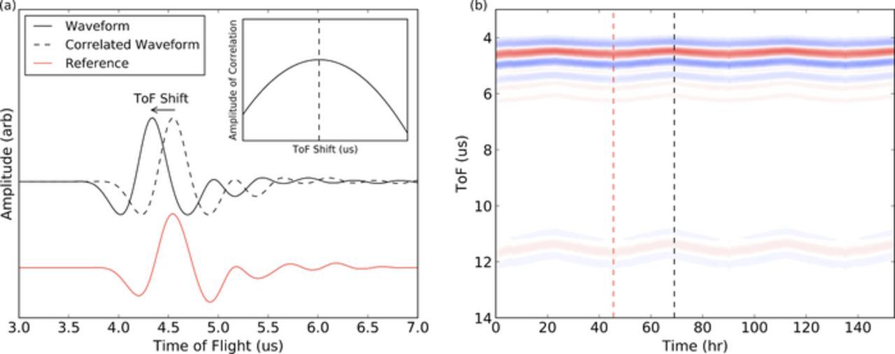
Figure 2. (a) The time of flight determination technique. The ultrasonic signal is correlated with the reference signal for all time shifts τ. The point of best correlation (τ where the integral is a maximum) is taken to be the time of flight shift for that state of charge of the battery, as schematically shown in the inset. The red waveform represents the reference signal, while the black waveform represents the correlated signal. (b) Heat map showing the evolution of the ultrasonic signals transmitted through a cell as it cycles. The red and black dotted lines represent the point in time at which the reference and correlated waveforms shown in figure (a) are taken. The red dotted line is the waveform in red shown on the left. The blue and red shades on the heat map represent the negative and positive amplitudes of the snapshot, respectively.
The total signal amplitude was also measured. This was determined by integrating the absolute value of the signal amplitude over the full waveform, as shown in Equation 12. As the signal amplitude at the beginning and end of the measured window is effectively zero, the contribution to amplitude change from waves shifting into and out of the measurement window is negligible. Therefore, this metric measures changes in the waveforms in the region of interest.
![Equation ([12])](https://content.cld.iop.org/journals/1945-7111/164/12/A2746/revision1/d0012.gif)
where A is the total amplitude of the waveform, f(t) is the waveform, and ti to tf is the waveform measurement window.
To predict states of charge and states of health from a large quantity of data, we use a supervised learning (machine learning) technique. We utilize the Support Vector Regression (SVR) method.18 Machine learning techniques require a training set, which consists of a feature vector (the input vector), and the desired output. In this case the inputs consist of combinations of the measured data: the acoustic data, either as a reduced ToF shift and/or total amplitude, or the complete waveform, and the voltage data. The input data was conditioned by normalizing the data for each cycle between 0 and 1. Where full waveforms were used for training, the data was normalized between −1 and 1. For the training set, the 'output' data consists of the variable that is to be later predicted, in this case the state of charge of the cell. The algorithm is trained on data from two cells, and the resultant transfer function is used to predict the state of charge on the third cell based on the selected input data (combination of tof, amplitude, waveform and voltage). Figure 3 illustrates a schematic of the methodology used for training the model and predicting SOC.
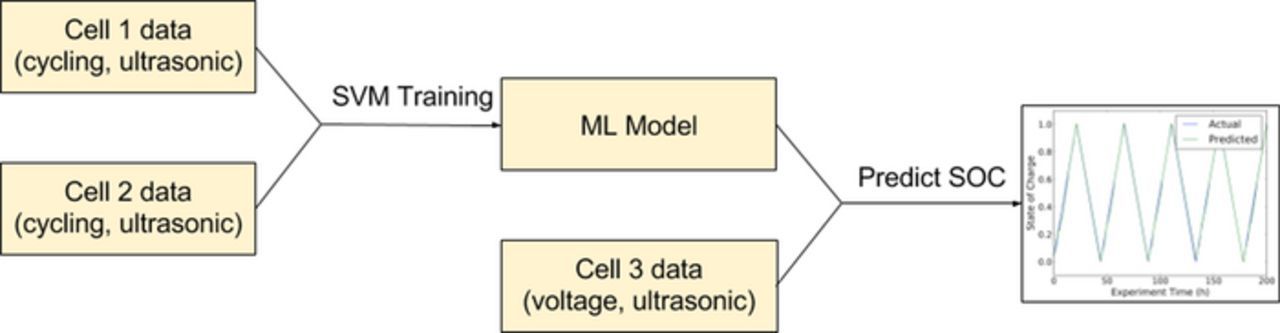
Figure 3. Schematic of the machine learning and SVM training technique for SOC prediction. The algorithm is trained on the data from two cells, and the ML model is used to predict the SOC for a third, independent cell.
Results and Discussion
State of charge and trends in ultrasonic signals
During cell cycling, clear and repeatable trends are evident in the ultrasonic waveforms, which vary periodically, synchronized with the electrochemical cycling. Figure 4 highlights this strong relationship between the ultrasonic signals and the state of charge of the battery for a LiCoO2/graphite (LCO) pouch cell. The most apparent trend during cycling is the bulk waveform shift, seen clearly in the ToF map in Figure 4a. As the cell charges, the bulk waveform shifts to a lower ToF (seen as the wave moving upward during charge in the top image of Fig. 4a), and shifts again to a higher ToF as the cell discharges. A hypothesis for the reasons for the ToF shifts will be presented later in this paper.
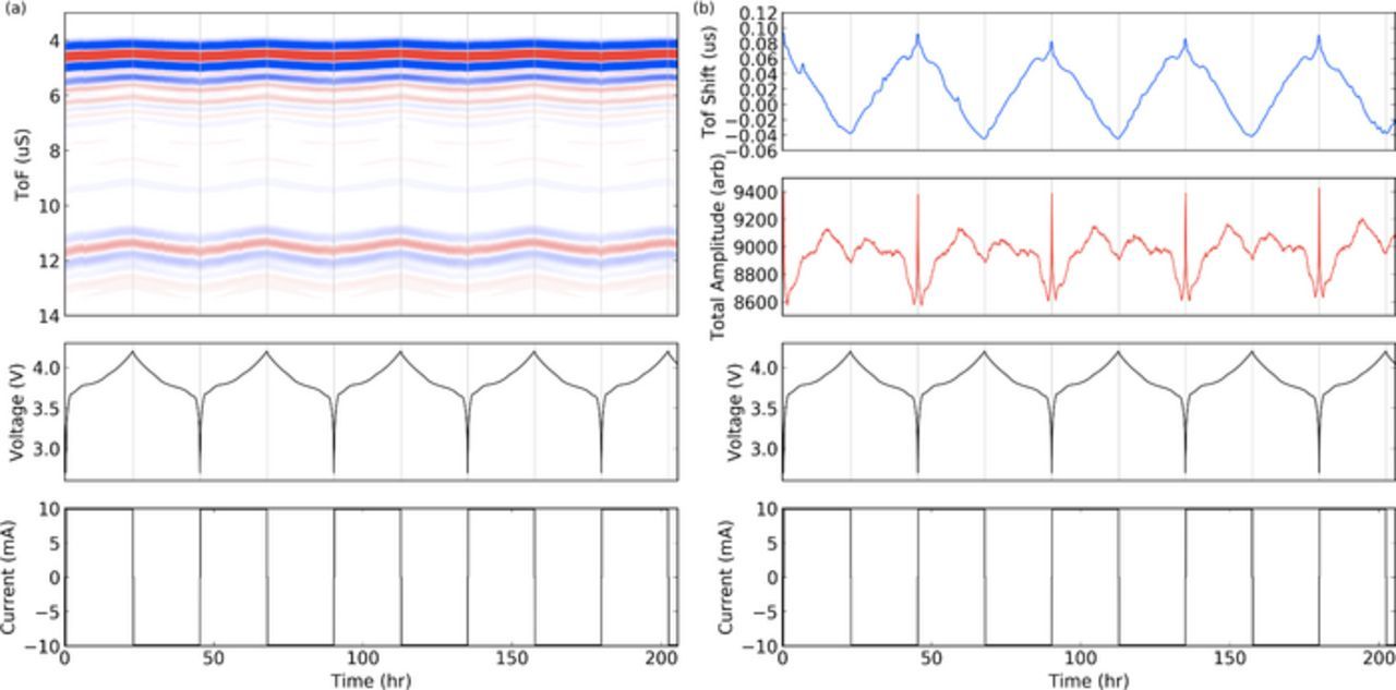
Figure 4. (a) Representative ultrasonic signal during cycling for several cycles of a LCO pouch cell at a C/20 charge/discharge rate. The TOF heat map shows maximum and minimum waveform amplitudes in red and blue respectively. (b) The same ultrasonic data reduced to a time of flight and amplitude metric. The blue and red lines represent the single TOF shift and amplitude measures respectively.
Figure 4b shows the full waveform data reduced to simpler ToF and signal amplitude metrics, using the cross correlation and integration techniques as described above. These metrics more clearly demonstrate the shifts that occur during cycling, demonstrating their repeatable and periodic nature.
Figure 5a shows the relationship between ToF shift and state of charge for a single, representative cycle. Progressing from top of charge, the overall waveform time of flight increases as state of charge decreases (discharging), and the overall waveform ToF decreases as the state of charge increases again (charging). A hysteresis is apparent in the signal during any given charge/discharge cycle. Toward the end of discharge there is an interesting observation: the ToF shift plateaus and undergoes a "double-dip" pattern, prior to rapidly spiking as the cell discharges to 2.7 V (i.e., capacity → 0 mAh). Figure 5b shows the signal over 60 cycles. The same general trend is apparent during each cycle. One noticeable evolution over cycles is the shift of the signal to higher ToF across the complete charge/discharge cycle. This overall shift to higher ToF will be discussed later in this paper, where we will discuss some observations between these overall time shifts and the state of health (SOH) of cells.
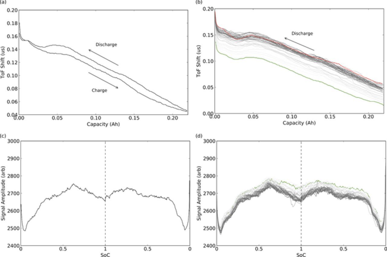
Figure 5. (a) A typical ToF shift vs state of charge curve. ToF increases during discharge. Hysteresis is apparent between charge and discharge. (b) ToF evolution for 60 cycles. Only discharge shown. Overall ToF increases for the whole range of SOC as cycle number increases. The green color represents the first of the cycles, and the red color the final cycle. (c) Typical amplitude profile during charge and discharge, and (d) amplitude evolution for 60 cycles. All data is from a LCO pouch cell.
Similarly to the ToF shifts, we see intra-cycle repeatable trends in the total signal amplitude for the LCO cell in Figures 5c and 5d. These show typical amplitude measurements during charge and discharge, and the overall evolution of amplitude over cycles. Of particular note is the significant drop off in amplitude below approximately 25% of SOC, followed by a spike in amplitude at bottom of charge. The significant and rapid change in the ToF shift and signal amplitude at bottom of charge indicates that significant structural changes are occurring at this level of discharge. This is a particularly strong indicator of over-discharge of a cell. Monitoring the combined ToF shift and amplitude measurements for this rapid change could be used to signal the beginning of over-discharge in battery management systems. Looking at signal amplitude across cycles, signal amplitude is seen to fade slightly as cycles increase.
The repeatability of the time of flight shifts and the signal amplitude provides an opportunity to use these features to accurately predict the state of charge of a cell. The intra-cycle electrochemical changes, and therefore mechanical properties of the material, give rise to the shifts that are seen in the ultrasonic waveforms during cycling. It is ultimately this electrochemical-mechanical coupling that gives rise to this prediction ability from the ultrasonic signals. Furthermore, given that the material properties shift continuously through cycling, this gives rise to an ability to distinguish clear changes in the material state, even when electrochemical measures, such as voltage, only show very small changes. Following the state of charge prediction discussion below, we further discuss the basis for the signal changes as state of charge varies.
Predicting state of charge using machine learning algorithms
We have shown that there are repeatable trends both in the time of flight shifts and total signal amplitude with respect to the state of charge of the battery. The same trends exist across multiple cells, however cell variability and noise during measurement results in some variation in the overall signal. This cell variation can present some challenges for direct inference of SOC with respect to inputs of amplitude and time of flight shift. With an aggregation of the available measured data: amplitude, time of flight shift and voltage, it is possible to make an estimation of the SOC of a battery despite these experimental and cell batch variations.
We use the Support Vector Regression (SVR) machine learning technique, as described in the Experimental section, to learn and predict state of charge of a lithium ion cell. Natural variation in cell performance2,11 and noise in the signal measurements makes direct linear regression challenging for accurate state of charge prediction. For instance, in Figures 4b and 4d, note the slight variations in the ToF shift and amplitude trends versus SOC between cycles. This, therefore, lends itself to machine learning techniques.
Data was used from three cells, which consisted of the measured parameters: voltage, waveform time of flight (ToF) shift and total signal amplitude, and the target measure: SOC. The algorithm was trained using two cells, and the state of charge was predicted on the third, independent cell. This was important to provide independent verification of the algorithm accuracy, without the algorithm having been trained on the predicted cell. Predictions of SOC were made at each point in time for which an ultrasonic snapshot was taken. Aside from the normalization of the ToF shift and amplitude between 0 and 1, the algorithm uses only the information provided at that single point in time: no information is used from previous points in the cycling to predict the instantaneous SOC for the independent cell, unlike coulomb counting or some other battery SOC monitoring techniques. Therefore, and importantly, the measurement is not history dependent. This is particularly important for robust SoC determination techniques that do not depend on the discharge history or conditions of the cell.
To compare the benefits of using acoustic data for determining state of charge, machine learning was applied using different combinations of the available inputs: voltage, time of flight shift and total signal amplitude.
Figure 6 shows the true state of charge and the predicted state of charge from the ML for several representative cycles. The least accurate predictions were those using voltage alone (Fig. 6a). Fundamentally, predictions using voltage alone are challenging, as voltage profiles shift over time (voltage fade), and changes in current result in variable overpotentials related to ohmic impedances, which can also vary with time. Figure 6b shows how the accuracy of the SOC determination was significantly improved using time of flight, signal amplitude, and voltage as inputs.
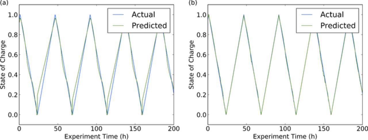
Figure 6. Representative prediction of state of charge (a) using only voltage inputs (b) using ToF shift, amplitude and voltage inputs to a machine learning model.
To quantify the improvements in SOC prediction, we calculated the errors in the state of charge determination by comparing predicted and actual SOC across the complete cycling history. The results for the LCO cells are shown in Figure 7a. The mean error of state of charge predictions is ∼3% using only voltage inputs. A slight improvement is observed (∼3% to ∼2.3%) when using only time of flight and amplitude as inputs. This error is reduced to ∼1% when time of flight, amplitude, and voltage are used.
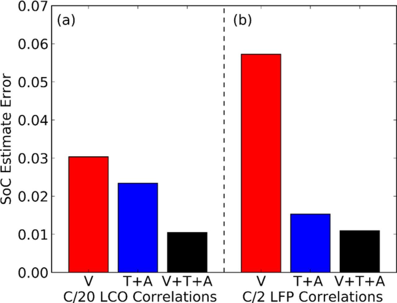
Figure 7. Errors of estimates using combinations of voltage (V), time of flight (T) and amplitude (A) inputs. (a) LCO pouch cell. (b) LFP pouch cell.
The same technique was applied to lithium iron phosphate (LFP) cell SOC prediction, and the resulting mean error is shown in Figure 7b. While state of charge prediction in LFP cells is particularly challenging due to the flat voltage profile and voltage hysteresis,4 the ultrasonic technique demonstrates that accurate predictions are possible using ultrasonic interrogation techniques. The mean error of state of charge predictions using only voltage inputs is ∼6%, which reduces significantly to ∼1% when using the ultrasonic ToF shift and amplitude inputs in addition to the cell voltage measurements. If used with more complex methods such as impedance measurements, it would be reasonable to expect that the accuracy could be further improved with the combination of physical and electrical methods.
Waveform shifts and material properties
The transmitted ultrasonic signal measured through the cell consists of several contributions. The bulk properties of the cell impact the propagation time of the wave: the materials in each layer, the stiffnesses and densities of these materials, and the layer thicknesses. The structure of the waveform, beyond the first-arrival time, will be impacted by the thickness of each layer and the relative properties of each adjacent layer.10 Here we consider changes that impact the first-arrival time.
As the cell cycles, the material properties within the anode and cathode change, including the modulus (stiffness) and density of the electrodes.14,19 In a pouch cell, where the geometry of the cell is loosely constrained, this also results in an overall cell thickness change. Together, the material and geometric changes result in a change in the overall propagation velocity of the ultrasonic wave, and this impacts the wave first-arrival time.
First we consider the influence of the overall cell thickness change on the time of flight response. For an unconstrained cell, the overall thickness varies during charge and discharge. Table I shows the thickness for a cell at several states of charge. During charge, the thickness of the cell increases: graphite expands as it lithiates, and LCO expands as it de-lithiates.14 This acts in the opposite direction of the time of flight shift shown in Figure 4b. An increase in thickness may be anticipated to increase overall time of flight, however, the time of flight decreases during charge. Therefore, we may draw the conclusion that while cell thickness changes may contribute to the the time of flight shifts, it is not the main contributor, and other more significant effects are at play.
Table I. Thickness change vs fully discharged state at various states of charge of an LCO pouch cell.
| SOC | 0 (Discharged) | 0.4 | 0.8 | 1 (Charged) |
|---|---|---|---|---|
| Thickness Increase (μm) | 0 | 0.011 | 0.107 | 0.154 |
Table II shows the material properties for graphite and lithium cobalt oxide as a function of degree of lithiation.14,19 As the cell discharges, the stiffness of the graphite decreases by a factor of >3, and the LCO stiffens by a factor of 2 (assuming full lithiation). Furthermore, the stiffness of the LCO does not change significantly until the degree of lithiation is >0.9, which occurs toward the end of discharge, depending on the lithium balance in the cell. As described by Equation 1, the wave propagation velocity depends directly on the stiffness of the material. A less stiff material will have a lower wave velocity. In addition, as graphite has a lower volumetric specific capacity than LCO,20 it takes up a larger volume in the cell and will have a larger impact on the overall wave propagation time and wave first-arrival.
Table II. Material properties for graphite and lithium cobalt oxide versus extent of lithiation.
| Graphite14 | LCO19 | ||
|---|---|---|---|
| Composition | Elastic Modulus | Composition | Elastic Modulus |
| LiC6 | 109 | Li0.5CoO2 | 89 +/− 3 |
| LiC12 | 58 | Li00.9CoO2 | 85 +/− 3 |
| LiC18 | 27 | Li0.95CoO2 | 96 +/− 6 |
| C6 | 32 | LiCoO2 | 178 +/− 5 |
Therefore to first order, as the cell cycles the graphite will have the largest impact on the overall velocity of propagation of the wave. Thus, as the cell discharges, the overall wave-speed will reduce, resulting in a time of flight increase. This is consistent with what is seen experimentally (Figure 3).
We can extend the analysis to estimate time of flight shifts vs. state of charge. The anode and cathode electrodes are porous composites, consisting of active material, binder, conductive additive and electrolyte. We make the assumption that the electrodes are homogeneous over the scale of the ultrasonic wave, as the wavelength is larger than the individual electrode thickness. To determine the effective wave velocity and density in each electrode we build an effective media model. Combining the material stiffnesses above with other electrode properties (see Appendix), we develop a Hashin-Shtrikman bound (see Methods) on the material stiffnesses,15 and use this to determine primary wave velocities vs. SOC as presented in Equation 1.
An estimate of the balance of the cell was made based on the relative volume of the electrodes and their volumetric capacities. The graphite, LixC6 was assumed to be slightly in excess, lithiating in the range x = 0.85 to x = 0, from top of charge to bottom of discharge. The LCO, LixCoO2 was assumed to lithiate in the range x = 0.5 to x = 0.95 from top of charge to bottom of discharge. Tables AI and AII present the values used to determine the electrode properties for this theoretical model.
Table AI. Material properties for determining electrode compressional wave velocities vs SOC.
| Aggregated | Electrode Sound | |||||||
|---|---|---|---|---|---|---|---|---|
| Material | Cell SOC | E (GPa) | Poisson's ratio | K (GPa)f | G (GPa)f | Density (g/cm3) | Thickness (mm) | Velocity (m/s)i |
| Cathode | ||||||||
| LiCoO2 | 178a | 0.32b | 164.8 | 67.4 | 4.9c | |||
| Li0.95CoO2 | 0 | 96a | 0.32 | 88.9 | 36.4 | 4.86 | 1.720g | 3010 |
| Li0.9CoO2 | 0.11 | 85a | 0.32 | 78.7 | 32.2 | 4.81 | 1.720 | 2860 |
| Li0.77CoO2 | 0.39 | 87 | 0.32 | 79.9 | 32.7 | 4.70 | 1.722 | 2909 |
| Li0.69CoO2 | 0.59 | 89 | 0.32 | 81.3 | 33.3 | 4.56 | 1.734 | 2972 |
| Li0.5CoO2 | 1 | 89a | 0.32b | 82.4 | 33.7 | 4.46f | 1.741g | 3018 |
| Anode | ||||||||
| C6 | 0 | 32b | 0.32b | 28.8 | 12.2 | 2.26d | 1.851g | 3884 |
| Li0.09C6 | 0.11 | 31 | 0.34 | 31.2 | 11.8 | 2.26 | 1.853 | 3282 |
| Li0.33C6 | 0.39 | 27b | 0.39e | 41.2 | 9.8 | 2.24 | 1.869 | 2583 |
| TabLi0.5C6 | 0.59 | 57.6b | 0.34e | 60.0 | 21.5 | 2.23 | 1.940 | 2510 |
| Li0.85C6 | 1 | 94 | 0.25 | 67.8 | 36.8 | 2.21 | 1.984g | 2498 |
| LiC6 | 109b | 0.24b | 69.9 | 44 | 2.20d |
aSwallow et al. (2014).19 bQi et al. (2014).14 cManufacturer Datasheet: LiCoO2 for thin film battery applications.21 dDoh et al. (2011).22 eQi et al. (2010).23 fCalculated. gExperimentally measured data.
Figure 8 shows the experimental time of flight shift overlaid with the time of flight shift versus state of charge calculated for the lithium ion pouch cell using material properties from literature combined with the analytical effective medium model, as described in the Methods section. The trends for the calculated model are very similar to the trends seen from the experiment. From the top of charge (SOC = 1), the ToF increases as the cell discharges. This is predominantly related to the graphite becoming less stiff as it delithiates. The stiffness change is related to the stronger ionic interactions from the lithiated graphite giving way to weaker van der Waals interactions14 as lithium is removed from the structure. As the cell reaches approximately 80% discharge (SOC = 0.2) the time of flight rolls over and begins to decrease. This is related to the LCO rapidly stiffening as extent of lithiation increases above x = 0.9 for the LixCoO2 cathode. At that state of charge the graphite is only changing in stiffness a small amount compared with the LCO.
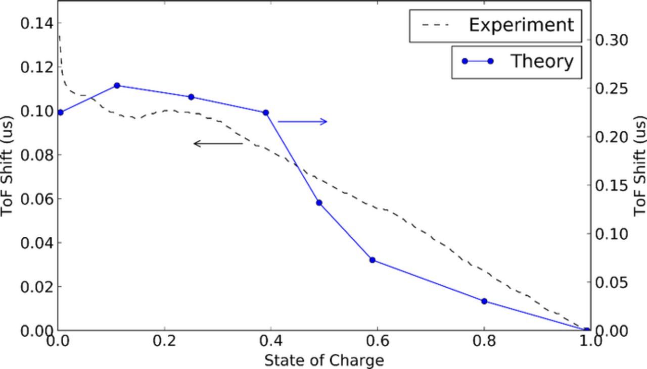
Figure 8. Experimental data (black dotted line) and theoretically calculated (blue line) time of flight shift.
The significant increase in time of flight at bottom of charge is not seen in this calculation. Further study is required to determine the mechanism for ToF spike, however it may be related to the full delithiation of the graphite as the battery reaches bottom of charge. In addition, the magnitude of the ToF shift calculated varies from the experimentally determined values for several possible reasons: the stiffnesses calculated using the H-S bounds is an estimation, and the actual values may differ. For instance, it does not take into account Backus layering effects which can impact wave velocity, as described above. Furthermore, errors in our estimated degree of lithiation would affect the calculated stiffness change. However, in each of these cases the trend of increasing ToF with decreasing state of charge holds.
Predicting state of charge of damaged cells
Extending the state of charge prediction analysis further, we consider cells which have been subjected to a protocol which has resulted in cell damage. The goal is to explore if state of charge can accurately be predicted on cells which have suffered damage, but for which the machine learning algorithm has not been explicitly trained.
We take cells with a known 106 cycle history, and state of health (SOH) of > 98%. Here SOH is defined as the remaining cell capacity divided by the initial cell capacity. The cells then underwent a low impedance closed circuit over-discharge event, reducing the cell voltage to almost zero volts. Following continuation of cycling, the cells are damaged, losing a significant proportion of capacity (∼10%), and then continuing to fade at a faster rate than prior to the damage event. Significant shifts in the ultrasonic signal are apparent following the failure (Figure 9).
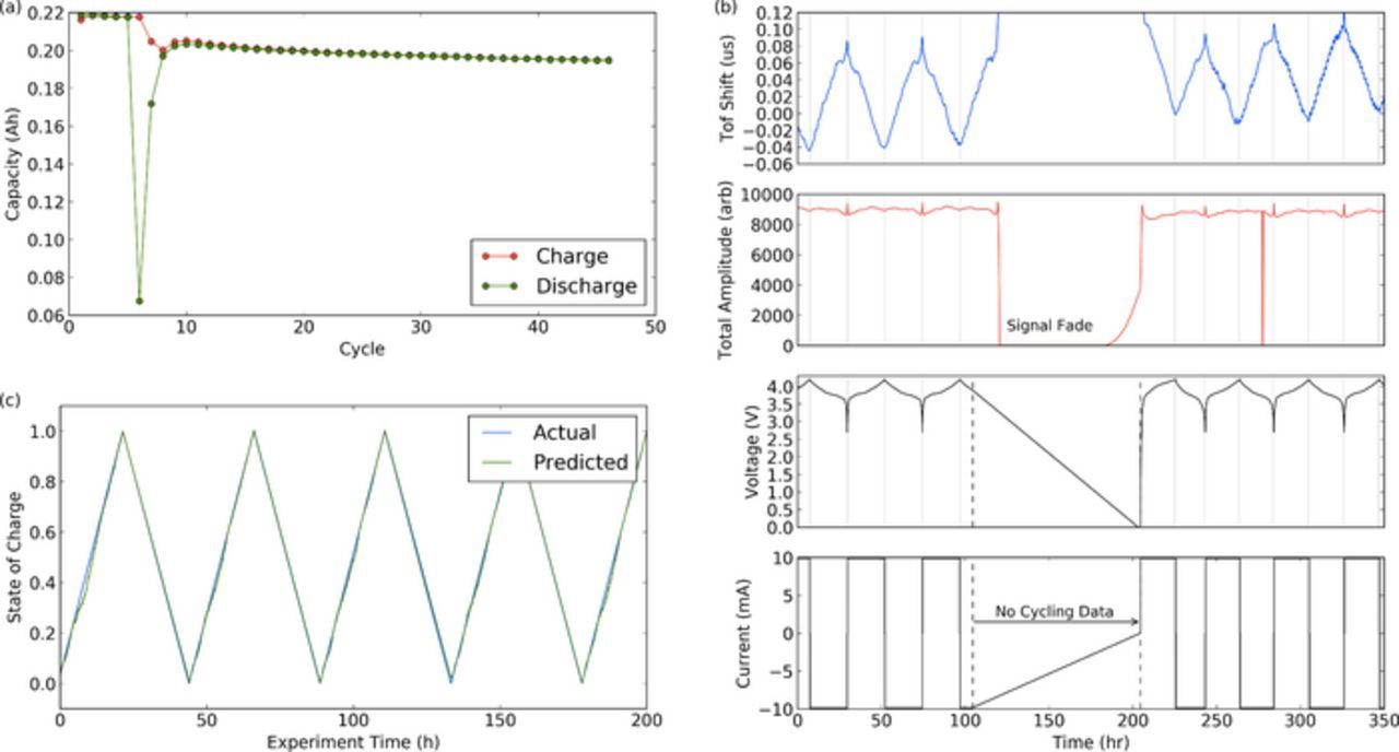
Figure 9. (a) The cell capacity before and after the cell damage, showing significant loss of capacity (b) the ToF and amplitude signals before and after cell damage. Note the cell voltage near zero following the failure, and (c) the prediction of state of charge following damage based on the ML algorithm trained only on healthy cells.
The machine learning algorithm, which has only been trained on "healthy" cells, is then applied to the cells to predict state of charge. While not as accurate as the prediction solely on undamaged cells, the estimate using voltage, signal amplitude and ToF still shows excellent correlation with the true state of charge of the battery, falling within ∼1.6% mean error. This compares with a mean error of ∼3% for the prediction using voltage alone. Therefore, the machine learning technique shows significant robustness for predicting state of charge, even in the event of unexpected and untrained cycling histories.
Figure 9a shows the cell capacity vs cycle. Cell damage is seen after 5 cycles in the Figure (previous 101 cycles not shown), and never returns to its previous capacity. Figure 9b shows the time of flight and amplitude shifts that occurred as a result of the failure. A region of cycling data is missing during the cycler failure, however the voltage is near zero on recommencement of cycling. The ultrasonic signal amplitude fades significantly following cycler failure, once the cell passes the typical bottom of charge. This is likely due to electrolyte breakdown and cell gassing. Figure 9c shows predictions for the state of charge of the cell following the damage. Despite the algorithm only being trained on undamaged cells, the predictions show good agreement with the actual SOC of the cells.
State of health metric
The ability to predict SOC following cell damage indicates that material changes within the battery structure which impact the ultrasonic signal, may also be used to predict the state of health (SOH) of a battery. We take three 210 mAh LCO cells cycled at a C/2 rate for 300 cycles, and use these as a dataset for SOH prediction. Neither the C/20 LCO or C/2 LFP datasets show significant enough capacity fade for SOH analysis.
The SOH is predicted using data from the top of charge of each cycle. No SOH predictions are made at intermediate states of charge. The inputs for this model consist of: i) time of flight shift referenced to a single cell reference signal (in this case, cell 1 at the top of charge during cycle 1); ii) total signal amplitude; iii) voltage; and iv) the complete ultrasonic snapshot. Each snapshot has the time of flight offset removed such that snapshots overlay each other and capture the evolution of the snapshot shape without the time of flight shift. The ultrasonic snapshot was normalized to the range [−1,1], and the remaining parameters were normalized to the range [0,1]. Training and testing was completed on independent cells, following the same protocol as was described earlier.
Figure 10 shows the actual (blue) vs predicted (green) state of health for the three LCO C/2 pouch cells. For each cell, the model was initially trained on data input from the other two cells. This trained model was then used to predict the SOH of the third cell. The first 20 cycles during cell break-in were not used for training and prediction because cell capacity changes rapidly during this time, making predictions challenging. Significant capacity spread and evolution exists between these cells, resulting in some variation in the predictions. However, the SOH predictions remain excellent, showing mean errors in the range 0.5–1.9%, with an average error across the cells of just over 1%.
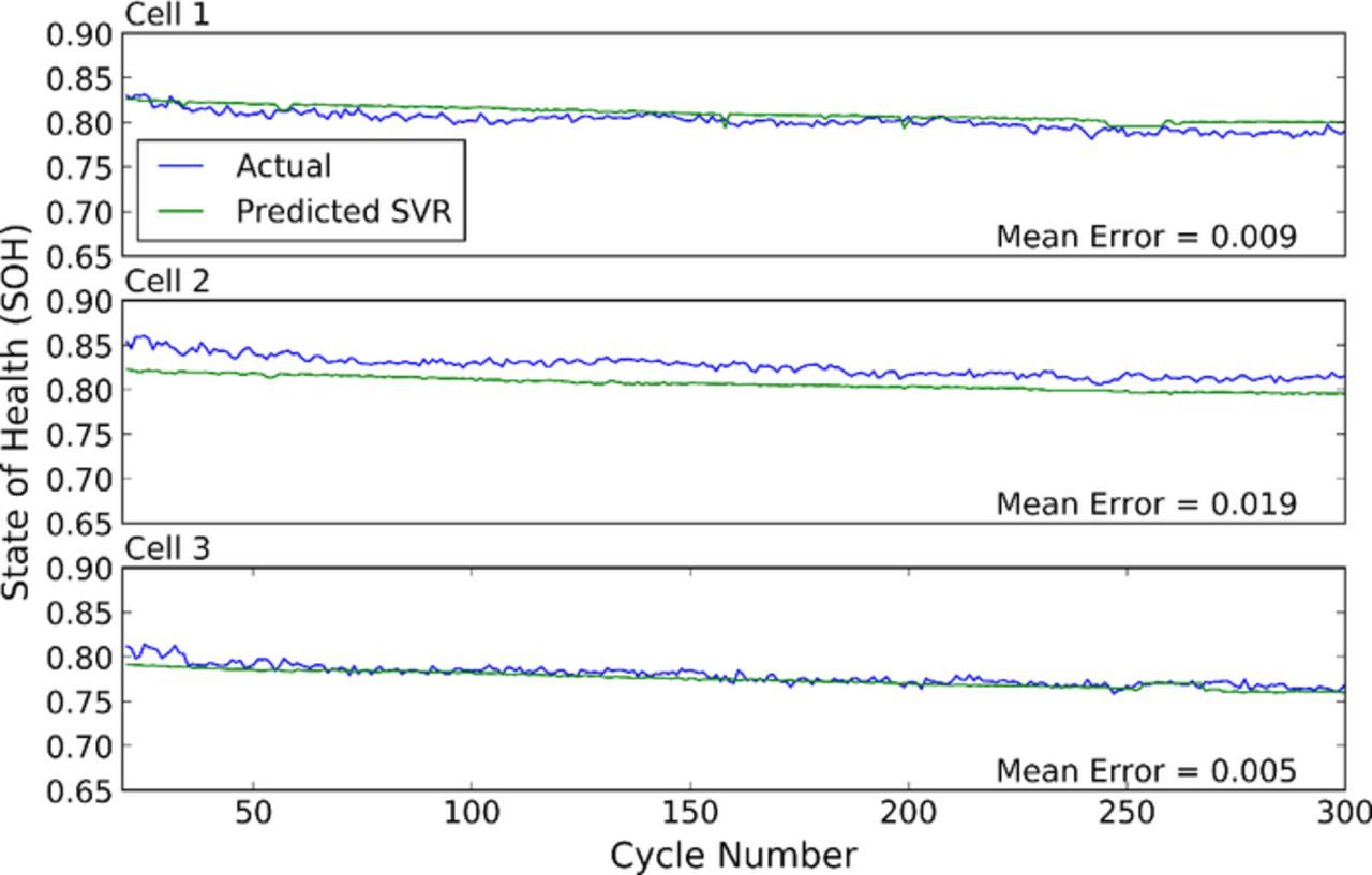
Figure 10. Actual (blue) vs predicted (green) state of health for three LCO cells discharged at a C/2 rate. The machine learning algorithm is trained on two cells, and then tested on a third, independent cell.
The predictions are startlingly accurate, particularly given the variability in the performance of the cells over time. This indicates that the ultrasonic signal is sensitive to structural differences in the cell, which give rise to changes in the state of health. This motivates potential uses for ultrasonic methods for second life, pack refurbishment, and faulty cell identification. It should be noted that this prediction only requires a single ultrasonic measurement in time, at top of charge, to predict SOH. No cell history knowledge is required, making this a powerful technique.
Conclusions
In this work we have shown that by using ultrasonic measurements and a machine learning model, we can accurately predict cell state of charge and state of health. Based on the hypothesis that the periodic ultrasonic trends could be used to predict cell state of charge, we used simplified time of flight and total signal amplitude metrics, along with the cell voltage, to train a simple machine learning (ML) model. We have shown that such a model can be used to predict a cell's state of charge to within an average error of ∼1%. This is a significant improvement over using the cell voltage alone in the ML model, which results in an average error of ∼3% for lithium cobalt oxide cells and ∼6% for lithium iron phosphate cells.
The same machine learning model was extended to predicting the state of charge of damaged pouch cells. We were capable of accurately predicting the state of charge despite the ML model not having been trained with data from damaged cells, demonstrating the robustness of the ultrasonic method. We concluded that the changes in time of flight can be attributed to changes in the material properties with state of charge.
Finally, we demonstrated estimation of the state of health of cells using another machine learning model with an expanded set of input data. Using the full ultrasonic waveforms at top of charge, in addition to the time of flight shift, total signal amplitude and cell voltage, we were able to predict the state of health of LCO pouch cells cycled at C/2 on average to within ∼1%. Despite significant variation in the performance of this batch of pouch cells, on an individual cell basis, errors varied in the range 0.5–1.9%.
Acknowledgments
This work was supported by DOE ARPA-E DE-AR0000621 and the Princeton University Andlinger Center For Energy and the Environment/Exxon Charter Award.