Is There a Benefit in Employing Graded Electrodes for Lithium-Ion Batteries?

Yanbo Qi; Taejin Jang; Venkatasailanathan Ramadesigan; Daniel T. Schwartz; Venkat R. Subramanian

doi:10.1149/2.1051713jes

Modeling and mathematical optimization can significantly improve the efficiency of battery design, helping to meet the growing demands for various applications. The idea of using modeling for battery design was first introduced by Tiedemann and Newman in 1975.¹ They used an ohmically limited porous electrode model to maximize the cell's effective capacity by changing the electrode thickness and porosity. Newman later applied the reaction-zone model to maximize the specific energy of the system, taking mass into consideration as well.² For these two models, the objective function can be directly related to the design variables, thus the optimum can be obtained by simply observing the plot or from the analytical solution. They further optimized the thickness and porosity of a lithium iron phosphate³ electrode, where they maximized the specific energy using the Ragone plots. Ramadesigan et al.⁴ went one step further by including the linear electrode kinetics to minimize the internal resistance of the electrode. They used control vector parameterization (CVP) to minimize the ohmic resistance in the positive electrode by varying porosity.

With the development of battery modeling, more physical processes have been included, and one of the most popular physics based models is the pseudo-2-Dimensional (P2D) model developed by the Newman group.⁵ The P2D model involves a set of nonlinear partial differential equations (PDEs) that can only be solved numerically. Therefore, a numerical optimization approach is required to perform optimization on the system. Du et al. proposed a surrogate-model-based approach,⁶ and later developed a sophisticated framework based on this approach⁷ with a gradient-based sequential quadratic programming optimization method. They applied the framework to a lithium manganese oxide electrode and investigated the effect of discharge rate, electrode thickness, porosity, particle size, and solid-state diffusivity and conductivity on the specific energy and power density of the battery cell. Golmon et al.⁸ extended the P2D model by incorporating the mechanical stress-strain relationship to account for the degradation due to cracks on the electrode particles. Thereafter, they developed a systematic framework to formulate the multi-objective and multi-design-parameter optimization problem with adjoint sensitivity analysis to reduce the computational cost.⁹ Another attempt along the line of faster optimization was done by De and his coworkers.¹⁰ They used a reformulated model developed by Northrop et al.,¹¹ with greatly improved the computational efficiency, and performed simultaneous optimization of multiple design parameters including the thickness and porosity of the positive and negative electrodes to maximize the specific energy of the cell. Xue et al. used an alternative way to do the optimization more efficiently by using an effective optimizer.¹² They applied the gradient-based algorithm framework to optimize the cell design to maximize the energy density with specific power density requirements for a spinel manganese dioxide cathode and meso-carbon micro beads anode system.

More recently, Dai and Srinivasan revisited the idea of using graded electrodes to achieve better performance.¹³ They used a gradient-free direct search method to maximize the specific energy under a certain discharge time by varying the design parameters such as electrode porosities and thicknesses, and compared the cases of uniform porosity and the graded electrode. They concluded that no significant improvement was observed by using the graded electrode design from their simulation. Later, Du et al. examined the effects of several design parameters, including graded porosity, on the performance of thick electrodes by simulation. They proposed several continuously changing porosity profiles in opposed to the more practical layered approach, and confirmed Dai and Srinivasan's conclusion that graded electrode design can only improve the performance slightly.¹⁴

In general, optimization approaches can be classified as indirect and direct approaches. The indirect approaches are also known as the variational approaches, in which the traditional necessary conditions from Pontryagin's maximum principle¹⁵ will be obtained for optimality. Since porosity is always bounded, it is difficult to apply indirect methods for this optimization problem. Alternatively, the direct approaches discretize the original optimization problem before solving it. There are two main subcategories of the direct methods: sequential and simultaneous approaches.

Most of the aforementioned optimization work used the gradient-based or gradient-free sequential optimization approach. The sequential approach takes the differential algebraic equation (DAE) system describing the physics, applies a certain linear or nonlinear programming (NLP) solver to them, discretizes only the control variables (partial discretization), and solves the model. Because it discretizes only the control variable, it is also known as the CVP method. At every iteration, a solution with a specific set of control variables is obtained. The optimal solution will be arrived at over multiple iterations. Note that as of today, global optimization cannot be guaranteed when CVP-type methods are used with P2D-based battery models.

The simultaneous approach, on the other hand, discretizes both the control variables and the design variables (full discretization) before solving the problem. When used for optimization, the DAE system will only be solved once at the optimal point, compared to the repeated numerical integration needed for the sequential optimization. By using higher order discretization scheme on both the state and the design variables, simultaneous optimization approach results in the faster determination of the optimum with fewer iterations.¹⁶ Furthermore, this approach offers more flexibility over constraints on the state variables. Since the state variables are also discretized, it is possible to apply equality/inequality constraints on their internal values directly.

In this paper, an ordinary differential equation (ODE) system (DAE system without algebraic equations) was involved due to the simplicity of the model. A general optimization framework based on a boundary value problem (BVP) with ODEs can be expressed as:¹⁷

with boundary conditions:

subject to bounds:

where

ϕ	Objective function
F	Differential equation constraints
	Vector of differential state variables
	Vector of control variables
	Space-independent parameters

In this paper, we will exam the performance of simultaneous optimization approach in the optimal design of battery electrode using a secondary current distribution model for the positive electrode. We will also compare its performance in speed and accuracy with the commonly used sequential approach.

Choice of the Model: Resistance Model for Battery Electrodes with Nonlinear Kinetics

While in the past we have used P2D model for design purposes¹⁰ and have published on efficient simulation of P2D models,¹¹ in this paper, we revisited the simple resistance model for battery electrodes keeping the independent variables to just 1D (x in this case). Use of P2D models means including at least one more independent variable (t) and possibly the independent variable for the radial direction (r). As of today, collocation methods as used in this paper works very well for ODEs. While there is progress in pseudo-spectral methods (collocation in x, t, and r), P2D models result in stiff systems of DAEs in time, which are challenging to deal with. Results of simultaneous optimization based on P2D models will be reported later. Note that just because a numerical method or scheme works well with a reasonable accuracy for solving a model, it does not mean that the same order of accuracy can be obtained for simultaneous discretization and optimization. Global Gauss collocation approach works well for 1D boundary value problems (BVP) problems, but finite difference methods lose accuracy and stability when used with the simultaneous discretization framework. P2D models might need more than global Gauss collocation for accuracy, possibly local collocation on finite elements in x, r, and t.

For a typical intercalation-based lithium-ion battery cell sandwich, the positive electrode is usually made of lithium transition metal oxide while the negative electrode is composed of lithiated graphite. During charging, lithium ions de-intercalate from the positive active material, travel through the separator, and intercalate into graphite the electrons travel in the opposite direction through the external circuit. During discharging, the reverse process takes place. In this paper, the mass transport process described above is considered to be fast and the intercalation/de-intercalation process is determined by the electrochemical reaction kinetics.

The positive electrode, as depicted in Fig. 1, is the main focus in this work. The x-direction is the direction of interest, which is along the thickness of the positive electrode, with x = 0 being the interface between the positive electrode and the separator and x = l_p being the electrode-current collector interface. The model used is a one-dimensional porous electrode model developed by Newman and Tobias.¹⁸ The following assumptions are made:

(1)
All variables such as potentials, current densities vary only along the thickness of the electrode, not in other directions (1-D).
(2)
There are no concentration gradients in the electrode. This assumption holds when charge/discharge process has just started from the equilibrium state, thus the concentration gradient has not had enough time to build up. Under this assumption, the model has no time dependency.
(3)
The double layer charging/discharging can be ignored.
(4)
The open-circuit potential of the positive electrode is assumed to be 0.

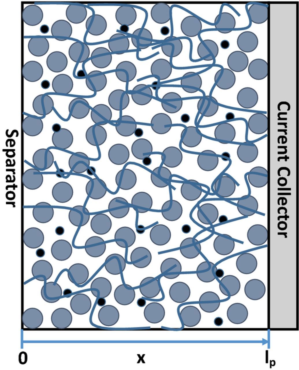
**Figure 1.** Schematic of the porous cathode being modeled. *x = 0 (X = 0 after nondimensionalization)* represents the boundary between the separator and the cathode, and *x = l_p (X = 1)* refers to the interface between the cathode and the current collector.

As there is no diffusion or convection in the system, all the current is carried entirely by migration. Therefore, the current density i₂, where the subscript 2 indicates the liquid phase (electrolyte), can be directly related to the migration flux: , where , and z_i is the charge number of species i, u_i is the electrochemical potential of species i, F is the Faraday's constant (96,487 C/mol), ɛ is the porosity, c_i is the concentration of species i, and Φ₂ is the potential in the liquid phase. Substituting the expression of into that of , we can arrive at the equation for the electrolyte conductivity

where the electrolyte conductivity .

Similarly, for the solid matrix, we have the equation for solid conductivity (Eq. 3), where the subscript 1 represents the solid phase and σ is the solid matrix conductivity.

The total current density for the whole system is the sum of the current densities in the solid and liquid phases.

From material balance, the change in concentration of lithium ions in the electrolyte is equal to the amount of ions transferred through the solid electrolyte interface:

where the active surface area (a, defined as surface area per unit volume) times the normal pore wall flux density of species i averaged over the surface area (j_in) gives the total flux of the species i transferred from the electrolyte to the solid phase.

From electroneutrality, the divergence of the total current density is zero, thus . An average transfer current density i_n for the system is defined as . Substituting it into Eq. 3 and Eq. 5, we got

The average transfer current density (i_n) is determined by reaction kinetics. Previously, linear kinetics was often used to simplify the problem:^1,4

where U stands for the equilibrium potential of the system. In this work, we have explored the influence of nonlinear kinetics on the electrode performance and its design, in which the equation above will be replaced by Eq. 8.

where n is 1 for lithium ion, α_a + α_c = 1 for the battery reaction; if we take U = 0 (assuming it is evaluated with a reference electrode of the same kind as the working electrode), then the equation for kinetics in the x-direction becomes

The final set of equations for the 1-D porous electrode resistance model consists of the following four equations:

One of the most important design parameters of the battery electrode is its porosity ε(x). The electrode porosity comes into effect through its influence on the material properties, such as the active surface area (for spherical particles), the solid phase and the electrolyte conductivities:¹

where ε_{f + p} is the volume fraction of the electrode filler and the polymer binder. The boundary conditions are:

Optimization Problem Formulation

Before applying the optimization approaches, the original DAE system has been further simplified to cut down the computational cost. In this case, the simplified DAE system becomes an ODE system without algebraic constraints.

The algebraic equation and i₂(x) can be eliminated by substituting i₂(x) = i_app − i₁(x) into the equation set 10. To facilitate the numerical simulation, nondimensionalization was conducted on x (), so that dimensionless distance X varies from 0 to 1. For the lithium intercalation/de-intercalation reaction, it is reasonable to assume symmetry by taking α_a = α_c = 0.5. After simplification, the model became:

For the resistance model that captures the ohmic resistance in both solid phase and electrolyte, as well as the charge transfer resistance associated with the reaction kinetics, one natural optimization objective would be to minimize the overall resistance of the electrode, which can be mathematically represented as:

SOCOLL Method

The specific simultaneous approach we will showcase here is the simultaneous optimization and collocation (SOCOLL) method proposed by Biegler.¹⁹ SOCOLL method uses the orthogonal collocation method to discretize both the control and state variables, before solving the problem at its optimal point. Collocation methods apply a polynomial approximation to the original differential equation. The zeros of the polynomials are called collocation points, where the differential equations should be satisfied. For a boundary value problem, the boundary conditions should also be satisfied at the end points.

The discretization of both control and state variables in scalar form can be expressed as:

where z_n, y_n, and u_n are the values of z(x), y(x), and u(x) at the n^th collocation point and P_n is a nth-degree polynomial.

Various kinds of orthogonal polynomials can be used with the SOCOLL method. In this study, we mainly used the interpolation polynomials in the Lagrange form, which can be written as:

Use of the Lagrange form facilitates solving only for the dependent variables at the collocation points as opposed to arbitrary constants in the polynomial representation. A detailed demonstration of how to apply the SOCOLL method and the traditional sequential approach to the electrode resistance model is described in the appendix.

All simulations and optimizations were performed using Maple 18 software classic worksheet in the 64-bit Windows 7 Professional environment on a Dell Precision T7500 work station with two 3.33 GHz Intel Xeon CPU and 24 GB RAM. The BVP solver used in this study is the "dsolve" function and the NLP solver is the "NLPSolve" function built in the Maple program for the sequential approach. Similar solvers and optimizers are available in other programs, e.g. the "bvp4c" and "fmincon" functions in Matlab. For the simultaneous approach, collocation approach was used.

For clarity, the variables and parameters of the resistance model (equation set 13) are listed in Table I.²⁰ The +/− sign for the current density implies its direction. A negative applied current density was used to represent the charging process. The value of the applied current density is at 1C to represent a typical one-hour charge.

Table I. List of Variables and Parameters in the Optimization Problem.

φ Objective function

F	Differential equation constraints
	Vector of differential state variables	[i₁(X), Φ₁(X), Φ₂(X)]
	Vector of control variables	ε(X)
	Bounds	u^L = 0.1, u^U = 0.7
	Space-independent parameters	Parameter²⁰	Symbol	Parameter values
		Electronic conductivity of the solid matrix	σ₀	3.8 S/m
		Ionic conductivity of the electrolyte	κ₀	0.98 S/m
		Particle radius of the active material	R_p	8.5 × 10⁻⁶ m
		Thickness of the electrode	l_p	144.4 × 10⁻⁶ m
		Inert material total volume fraction	ε_{f + p}	0.214
		Faraday's constant	F	96,487 C/mol
		Ideal gas constant	R	8.314 J/(mol·K)
		Temperature	T	298.15 K
		Applied current density	i_app	−23.12 A/m²
		Exchange current density	i₀	4.16 A/m²

Results and Discussion

Uniform porosity optimization

The conventional battery electrode is designed to have a uniform structure without property variation. The uniform electrode is easier to manufacture, and also easier to simulate and optimize. To optimize a uniform electrode without porosity distribution, ɛ can be treated as a constant variable independent of X, instead of the ɛ(X) in the equation set 13. Since porosity is now a constant variable, there is no need to discretize ɛ. The results from the simultaneous and the sequential approaches are listed in Table II. The bounds for the design variable ɛ are 0.1 ⩽ ε ⩽ 0.7 for both cases. An initial guess of 0.4 was given to the optimizer.

Table II. Uniform Porosity Optimization Using the Simultaneous (SOCOLL) and the Sequential (CVP) Approaches.

Approach	Number of collocation points	Optimization time (s)	Objective function φ (Ω-cm²)	Optimal porosity
Simultaneous (SOCOLL)	2	0.031	4.6199	0.3052
	3	0.046	5.3414	0.3413
	4	0.047	5.3503	0.3433
	5	0.063	5.3510	0.3435
	10	0.109	5.3510	0.3435
Sequential (CVP)	N.A.	0.250	5.3510	0.3435

From Table II, it can be observed that for this problem, the SOCOLL method converges for k = 5 internal collocation points. Both approaches returned the optimal porosity of 0.3435 and minimum resistance of 5.3510 Ω-cm². When using k = 5 for the SOCOLL method, it is 4 times faster than the CVP method. Since BVP method involves solving the equations at every iteration, it is expected to be slower compared to the SOCOLL method, where the equations are solved only once at the optimum.

Due to the relative simplicity of the resistance model and a small search space, it is straightforward and easy to evaluate the objective function over the feasible region. The result is shown in Fig. 2. From the plot, it can be seen clearly that over the feasible region of [0.1, 0.7] for porosity, the objective function resistance is convex, and the optimal point is consistent with the results from the SOCOLL and CVP methods. It should also be noted that the curve is relatively flat near the optimal point from 0.25 to 0.45, which covers most of the common porosities in commercial cells and in the literature, with around 8.6% difference in resistance in that porosity range.

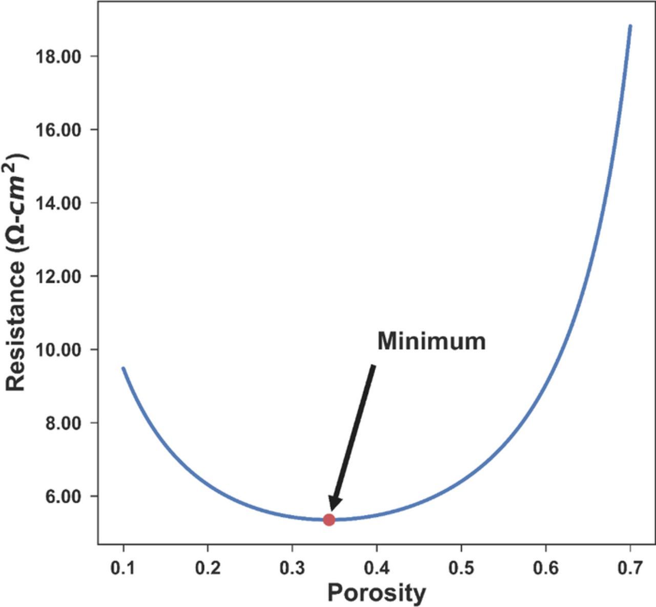
**Figure 2.** Resistance for the entire cathode as a function of different uniform porosity values. There is a single minimal resistance value in the feasible region for porosity varying between 0.1 and 0.7, making the optimization problem convex. The minimum is consistent with the optimal porosity of 0.3435 from both the sequential and the simultaneous approaches.

Since the Bulter-Volmer expression was used instead of the linear kinetics, the optimal porosity depends on the operating condition, the value of i_app in this case. The same optimization was carried out with i_app = 0.2C and 5C (value of 23.12 A/m² listed in Table I is at 1C), which covers most of the normal operating range for batteries. Optimal porosities of 0.3432 and 0.3480 were achieved, with the minimum resistance of 5.3610 Ω-cm² and for 0.2C and 5.1373 Ω-cm² for 5C respectively. Compared with the 1C case of 0.3435 being the optimal porosity, the difference in porosity is around 1%, below the controllable error in manufacturing. This is due to the relatively fast electrochemical reaction rate of the system. For the rest of the paper, 1C rate was used for optimization since the influence of C rate is small in this case.

Graded electrode optimization

The idea of using electrode with porosity distribution in model-based electrode design for lithium-ion batteries was first introduced by Ramadesigan et al.⁴ Golman and her colleagues⁹ also examined the effect of the graded electrode with mechanical properties considered. Recently, Dai et al.¹³ carefully looked at the performance improvement by utilizing a full P2D model and recommended the manufacturers not to make the graded electrode due to the additional processes involved and very small improvement achieved. In this paper, we want to quantify the gain in terms of electrode resistance with the two optimization approaches. This is a revisit to Ramadesigan's optimization problem, with nonlinear reaction kinetics instead of the linear kinetics assumption he made in his paper.

The simplest case for the graded electrode is a 2-layer porosity distribution structure. The original cathode can be divided into two regions of equal thickness and within each region, the porosity is a constant, as demonstrated in Fig. 3. For the sequential approach, the original ODE set was doubled with porosity being ε₁ and ε₂ in layer 1 and layer 2 respectively. The values for all state variables were set to be continuous across the layers. For the simultaneous approach, within each layer at each node point, the polynomial expressions for all the variables were substituted to the original ODE system. A 4.4% reduction in resistance can be obtained from using a graded porosity with 2 layers compared to uniform porosity.

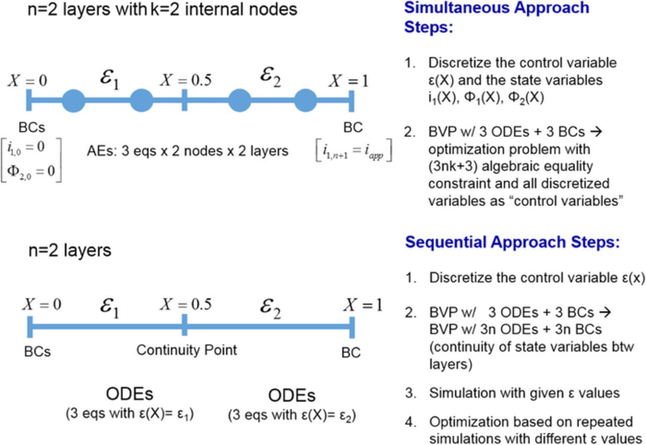
**Figure 3.** Demonstration of the 2-layer graded electrode optimization using the simultaneous approach vs. the sequential approach. The simultaneous approach discretizes both the porosity and the state variables Φ₁, Φ₂, i₁ for each layer. At every node point, there is a numerical value for each variable, and all these numerical values will be varied by the optimizer. On the other hand, for the sequential approach, each layer is represented by the whole set of the original ODEs with porosity substituted by a constant. The continuity point between the two internal layers refers to the continuity of the values of Φ₁, Φ₂, i₁.

Similar to the uniform case, a contour plot of the electrode resistance over the search space can be made to visualize the optimization problem, as shown in Fig. 4. The diagonal line of ε₁ = ε₂is equivalent to the uniform electrode case shown in Fig. 2. The area inside the contour of 5.3510 Ω-cm² in resistance represents the 2-layer graded electrode designs where resistance is no bigger than the uniform optimal case. Compared with a single point (ε = 0.3435) for the uniform electrode, the design space has been enlarged significantly (ε₁ ∈ (0.31, 0.52) and ε₂ ∈ (0.12, 0.36)) for the 2-layer graded electrode, providing greater freedom for other design considerations. It can be observed that the resistance values get larger for higher porosities, especially for bigger ε₂. The resistance model used only captures the ohmic resistance in the electrolyte and the solid matrix and the charge-transfer resistance associated with the Butler-Volmer kinetics. Since the electronic conductivity in the solid is higher than the ionic conductivity in the electrolyte (see parameters in Table I), the solid phase is more favorable compared to the electrolyte, thus the optimal porosity (porosities) is smaller than 0.5. The boundary condition at X = 1 forces the solid phase to carry all the current, thus lower porosity near the current collector, where the solid phase current is higher, is preferred to reduce the ohmic resistance. The optimization results from the two approaches are listed in Table III. Likewise, optimization for a graded electrode with more layers can be performed using these two methods, whose results are also listed in Table III.

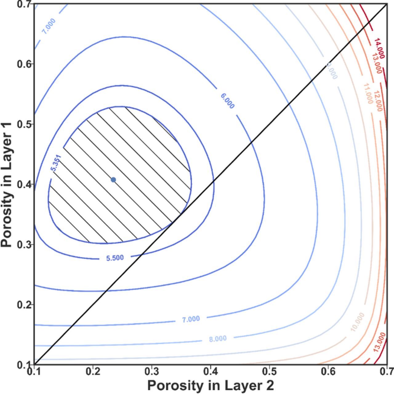
**Figure 4.** Contour plot for the resistance of a 2-layer graded cathode with different porosity combinations. Layer 1 is for X ∈ (0, 0.5), and layer 2 is for X ∈ (0.5, 1). The blue dot represents the point of minimum resistance (5.1164 Ω-cm²) for the 2-layer graded electrode. The diagonal line of ε₁ = ε₂ is equivalent to Fig. 2 for the uniform case with the intersection point with the 5.3510 Ω-cm² contour being the minimum. The hatched area inside the contour represents the search space for 2-layer graded electrode design with resistance no bigger than the uniform minimum case. By introducing the second layer of graded electrode, the feasible region changes from a point to a reasonably sized area. With the extra freedom in design, more objectives can be considered without resulting in an electrode with higher resistance.

Table III. Graded Electrode Optimization Using the Simultaneous (SOCOLL) and the Sequential (CVP) Approaches.

	Optimization time (s)		Objective function φ (Ω-cm²)		Optimal porosities
Number of
graded layers	Simultaneous (10 nodes each layer)	Sequential	Simultaneous	Sequential	Simultaneous	Sequential
1	0.109	0.250	5.3510	5.3510	0.3435	0.3435
2	0.266	5.663	5.1164	5.1164	0.4076;	0.4075;
					0.2347	0.2347
3	0.624	53.992	5.0605	5.0605	0.4267;	0.4267;
					0.3371;	0.3371;
					0.1820	0.1820
4	1.264	243.159	5.0372	5.0372	0.4347;	0.4353;
					0.3798;	0.3801;
					0.2866;	0.2875;
					0.1505	0.1507
5	2.137	690.570	5.0251	5.0251	0.4388;	0.4392;
					0.4014;	0.4027;
					0.3386;	0.3378;
					0.2505;	0.2502;
					0.1292	0.1286
∞	-	-	5.0034	-	-	-

All the results are based on the graded electrode of equally thick sub-layers. Allowing the thickness to vary together with the porosity can further reduce the resistance, but the improvement is not much for this problem. For example, for a 2-layer graded electrode, the minimum resistance with optimal thickness distribution is 5.1019 Ω-cm² (62.37% of the total thickness for layer 1 with a porosity of 0.3972 and 37.63% of the total thickness for layer 2 with a porosity of 0.1985). Compared with the minimal resistance of 5.1164 Ω-cm² for the equally distributed two sub-layers listed in Table III, the improvement is only 0.3%. Considering that keeping the thickness to be equal in each sublayer would be more practical for manufacturing and to simplify the problem, only the results for equally thick multi-layer graded electrode are shown in this work.

It can be observed from Table III that the optimization time for the sequential approach increases dramatically as more layers are used. This is due to the increased number of ODEs required to be solved at each of the porosity combinations. In contrast, the time needed for simultaneous approach did not increase as much, since increasing the number of algebraic equations in the optimization problem does not increase the problem complexity as much, particularly for sparse optimizers. For a graded electrode with more than 2 layers, Maple's built-in ODE solver "dsolve" does not work properly, so a customized Newton-Raphson solver was used with the collocation approach in x for solving the model.

Comparing the results from the two approaches, the optimal porosity profiles agree very well with each other. As the number of graded layers increases, the disagreement between the two approaches also grows slightly. This probably resulted from the fact that the search space is flat near the optimum, thus there are many combinations of the porosity values that give similar ohmic resistance. The main differences between the two approaches are listed in Table IV for clarity.

Table IV. Summary of the Key Differences Between the Simultaneous and the Sequential Approaches.

	The simultaneous approach	The sequential Approach
Discretized variables	Control + State variables	Only control variables
Requirements on the discretization scheme	High, needs high efficiency in choosing node points	Low, works with most discretization schemes
Requirements on the optimizer	High, needs to handle a large number of design variables	Low
Speed	Fast	Slow
Allow direct control of the state variables	Yes, can be handled as objectives or constraints	Partly, can only be handled approximately (by penalty or using variables evaluated at arbitrarily selected points)

From the perspective of reducing the resistance of the cathode, building graded electrode beyond 2 layers does not help much. Compared with the uniform optimal porosity, the reduction in ohmic resistance for 2-layer, 3-layer, 4-layer, and the 5-layer graded electrode is 4.4%, 5.4%, 5.9%, and 6.1% respectively. The limiting case is a continuously changing porosity distribution, with 5.0034 Ω-cm² in resistance, a 6.5% improvement compared with the optimal uniform electrode. Considering the additional processing time and cost for adding layers of different porosities, it is probably not cost-effective to manufacture a graded electrode, especially for more than 2 layers. It is worth pointing out that we did not keep the amount of the active material the same for the graded electrodes listed in Table III. However, the average porosities for 2-layer, 3-layer, 4-layer, and 5-layer graded electrode were 0.3214, 0.3152, 0.3135, and 0.3119 respectively, not far from the uniform optimal porosity 0.3435. With the same active material constraint, the minimal resistances for 2-layer, 3-layer, 4-layer, and 5-layer graded electrode are 5.1300 Ω-cm², 5.0976 Ω-cm², 5.0823 Ω-cm², and 5.0748 Ω-cm², which are slightly larger than the values in Table III.

If a conclusion was to be made just based on the results so far, it would confirm the conclusion from Dai et al.¹³ that graded porosity is not very useful. However, the next section will show the cases where graded design in the electrode is needed.

Constraints on the State Variables

Uniform electrode

Apart from the advantage in computational speed, which may not be critical for design since we can afford the time offline, one key advantage of the simultaneous optimization approach is that it allows control of the state variables directly. Owing to the fact that all the variables are discretized before applying the optimizer and that all the discretized numerical values are treated as "control variables", it is easier to give bounds and constraints on the state variables, just as the real control variables. This feature of the simultaneous approach can be very powerful and useful when internal state variables are important. For example, by controlling the overpotential at each internal node points, side reactions can be suppressed, which can be used to improve life performance. In the cases where optimization objective does not improve much compared with the base case (like the graded electrode), we can still use the simultaneous approach to control the state variables for the design.

For this secondary current distribution resistance model, a variable of great interest is the activation overpotential η(X) = Φ₁(X) − Φ₂(X). η(X) is the measure of the interfacial voltage difference above the equilibrium potential, which represents the driving force for lithium intercalation and de-intercalation in the positive electrode. When η(X) is larger, the intercalation and the de-intercalation process will be faster according to the Butler-Volmer reaction kinetics (Eq. 9), but at the same time, the rate for side reactions also increases. The side reactions are one of the main causes of battery degradation and are strongly dependent on the cell chemistry. For a lithium nickel cobalt oxide cathode, the formation of solid-electrolyte interphase (SEI) layer due to electrolyte oxidation and LiPF₆ decomposition accompanied by the evolution of gaseous species are the main concerns.²¹ The SEI layer growth in the carbon anode is believed to be responsible for capacity fade, while the interfacial impedance increase resulted from lithium nickel cobalt oxide cathode expedites power loss, especially at the high end of charge voltages when η(X) is large. Generally, a uniform distribution of low η(X) values across the electrode is desired to fully utilize the active material while reducing side reactions. To measure the uniformity of η(X) values, the standard deviation (SD) was used according to the following equation:

where is the mean of all the η(X) values.

As discussed earlier, to minimize the electrode resistance, an optimal porosity of 0.3435 for uniform electrode was determined. For the optimal uniform electrode, the mean and the standard deviation of η are 6.6834 mV and 2.0914 mV respectively. Thanks to the simultaneous optimization approach, the mean or standard deviation of η can be controlled directly when carrying out the optimization. An example to illustrate the ability to control the standard deviation of the overpotential is given below.

For the uniform electrode, the ohmic resistance of 5.3510 Ω-cm² in the optimal case had to increase in order to lower the standard deviation of the overpotential. An inequality constraint on the ohmic resistance

was added to the new optimization formulation to gently relax the constraint on the resistance. The new objective function is

where k is the number of internal node points (k = 30 was used to ensure convergence). The minimal value of 1.563 mV was achieved where the porosity was 0.4054 and the resistance was at 5.0823 Ω-cm². When the constraint on the resistance was completely removed and the only objective was to minimize the standard deviation of the overpotential, the minimal standard deviation of 0.7009 mV could be achieved. In that case, the porosity was 0.5529 and the resistance was 7.4563 Ω-cm². The plots for the internal variables of the aforementioned three cases are shown in Fig. 5. Compared with the minimal resistance case, to minimize the overpotential variance, the solid phase current was reduced in absolute value. Since more current was forced through the electrolyte, higher porosity is favored to lower the potential increase in the electrolyte. The slope of the solid phase current was increased in the two cases for overpotential standard deviation minimization. According to the Butler-Volmer equation (Eq. 9), as the slope increases, the overpotential also increases, which corresponds to higher curves in Fig. 5d when the standard deviation is smaller.

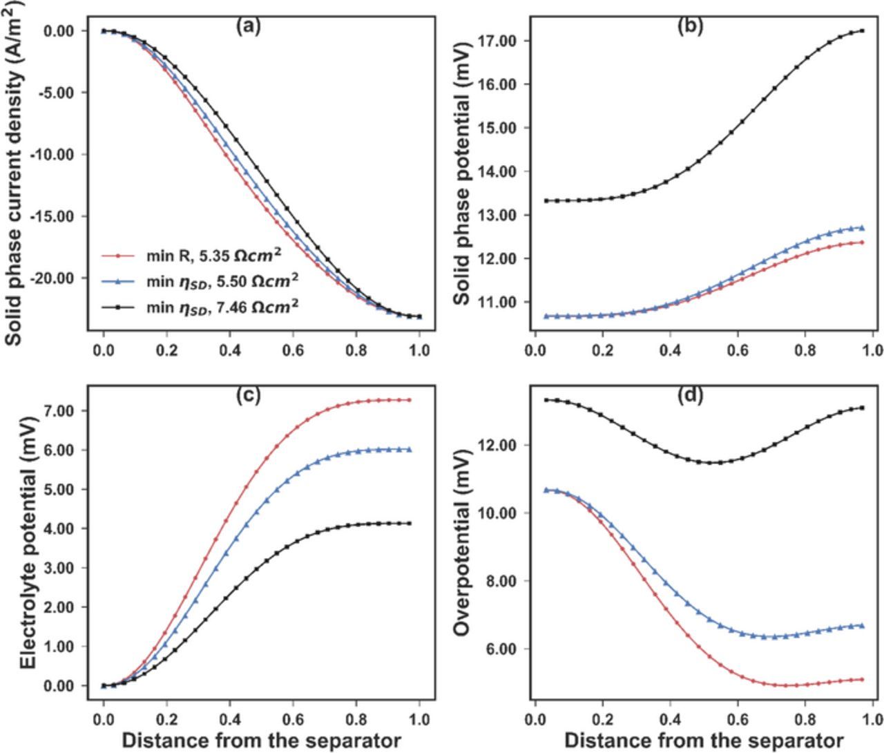
**Figure 5.** The internal profiles of (a) the solid phase current density, (b) the solid phase potential, (c) the electrolyte potential, and (d) the activation overpotential for three uniform electrode optimizations. In case 1 (red dots), the only objective is to minimize the overall resistance, and the minimal resistance is 5.3510 Ω-cm². In case 2 (blue triangles), the main objective is to minimize the standard deviation of the overpotential, with a constraint that the overall resistance is no larger than 5.5000 Ω-cm². In case 3 (black squares), the only objective is to minimize the standard deviation of the overpotential. The electrode resistance is evaluated at 7.4563 Ω-cm² for this case. These optimizations show the ability to control the profile of the internal state variables by using the simultaneous approach. A trade-off between the electrode resistance and the overpotential variance seem to exist.

With this optimization framework, a desired resistance value (greater than the minimal resistance) can be guaranteed while optimizing for other design considerations.

Graded electrode

From the uniform electrode case, it can be seen that there is a trade-off between the resistance and the overpotential variance. To lower the overpotential variance, a compromise on the resistance has to be made. This is where the graded electrode can come into play. With a greater search space as shown the shaded area in Fig. 4, it is likely that a smaller overpotential variance can be achieved without sacrificing the resistance.

The constraint

was added to the graded electrode optimization problem, where 5.3510 Ω-cm² is the minimum resistance for the uniform case. This constraint can ensure that the resistance of the multi-layer graded electrode does not increase compared to the best uniform case. The optimization results are listed in Table V. The hypothesis that by employing graded electrode the overpotential variance can be reduced without incrementing the electrode resistance was confirmed. The state variables for the optimal cases with 2 to 5 sub-layers are plotted in Fig. 6 together with the optimal uniform case. All 5 cases have the same electrode resistance of 5.3510 Ω-cm². Similarly, the most gain of bringing in the graded electrode design can be obtained with 2 sub-layers. In the limiting case of continuously changing porosity (infinite number of sub-layers), the minimal overpotential deviation with the resistance of 5.3510 Ω-cm² is around 0.9 mV.

Table V. Optimization of Graded Electrode to Minimize the Standard Deviation (SD) of the Overpotential while Maintaining the Same Resistance (5.3510 Ω-cm²).

Number of	SD of the	Average	Optimal
layers	Overpotential (mV)	overpotential (mV)	Porosities
1	2.0914	6.6834	0.3435
2	1.3934	7.5929	0.4643;
			0.3480
3	1.2426	7.5983	0.4528;
			0.4835;
			0.2880
4	1.1738	7.6235	0.4407;
			0.5093;
			0.4391;
			0.2477
5	1.0953	7.7251	0.4331;
			0.5100;
			0.5060;
			0.3963;
			0.1997

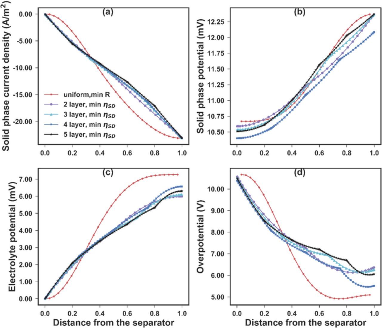
**Figure 6.** The internal profiles of (a) the solid phase current density, (b) the solid phase potential, (c) the electrolyte potential, and (d) the activation overpotential for multi-layer graded electrode optimizations. The red dotted lines, generated by minimizing the electrode resistance for a uniform electrode, were used as a baseline. For the 2-layer (purple pentagons), 3-layer (cyan triangles), 4-layer (blue squares), and 5-layer (black stars) graded electrode design, the main objective is to minimize the standard deviation of the overpotential while maintain the overall resistance to be at 5.50 Ω-cm², same as the baseline case (red dot). By introducing the graded electrode, it is possible to reduce the overpotential non-uniformity without increasing the resistance. Most gain by using the graded structure can be achieved with 2 layers.

From Fig. 6, it can be observed that for multi-layer graded electrode, the curves bend slightly across the boundary between layers. This is due to the fact that the potentials are plotted in Fig. 6. The currents, which are equal to the conductivity times the derivative of the potentials are not continuous across layers. Since the conductivities in the electrolyte and the solid matrix depend on the porosity (Eq. 11) and change across layers, the derivative of the potential should also change across the regions with different porosities.

Multi-Objective Optimization using an Evolutionary Algorithm

As discussed earlier, there is a trade-off between minimizing the resistance and reducing the overpotential variance. Furthermore, from Table V, a conflict in minimizing the overpotential variance and the average overpotential can also be observed. For a complicated electrochemical system like lithium-ion batteries, multiple criteria decision making is often encountered, such as the trade-offs between resistance, overpotential variance, and average overpotential in this resistance model.

Similar to Fig. 2, the average overpotential and its standard deviation with respect to a uniform porosity can be plotted, as shown in Fig. 7. The thermal voltage , where k_B is the Boltzmann constant (1.381 × 10^{− 23} m²kgs^{− 2}K^{− 1}), T is the temperature in Kelvin, and e is the elementary charge (1.602 × 10^{− 19} C), is 25.5 mV at room temperature (296.15 K). It should be noted that for the parameter set used in this problem (see Table I), the average overpotential is in the range of 5 to 30 mV, comparable with the thermal voltage at room temperature, which suggests that the full Butler-Volmer equation should be used, not the linearized version (for ) or the Tafel form (for ). This is consistent with the discussion earlier that the applied current is comparable to the exchange current.

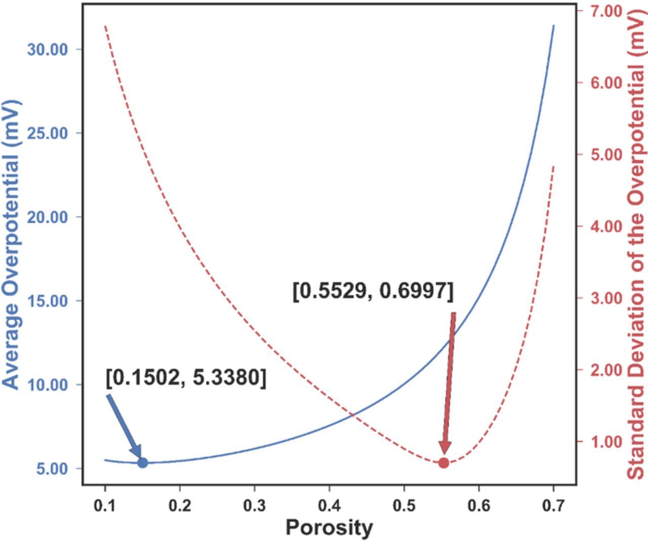
**Figure 7.** The change of average overpotential (blue solid) and the standard deviation of the overpotential (red dashed) as a function of the uniform porosity. The optimal porosity for the two objectives is 0.1502 and 0.5529 respectively. There is no single porosity value that can minimize both objectives at the same time, thus a multi-objective optimization is needed.

From Fig. 7, it is obvious that no porosity can simultaneously minimize both the average and the standard deviation of the overpotential, thus this is a non-trivial multi-objective optimization problem. For such a problem, instead of a single solution, a number of nondominated solutions, known as the Pareto-optimal solutions, exist. A solution can be called a Pareto-optimal solution when none of its objective functions can be improved without sacrificing another objective function. Without further information, the Pareto optimal solutions are considered to be equally good.

Various optimization algorithms have been proposed to solve multi-objective optimization problems, including the classical scalar approach of converting the problem into a single-objective problem by giving weights to each objective and the evolutionary vector approach of considering all the objectives simultaneously to find multiple Pareto-optimal solutions. In the previous section for applying constraints on the state variables with the simultaneous approach, the ɛ-constraint method was used.²² The ɛ-constraint method is a classical multi-objective optimization method. It converts the original multi-objective optimization problem into a single objective optimization problem with all the other objectives as constraints. In the previous section, the original optimization problem being minimizing resistance and the overpotential variance at the same time and the problem after applying the ɛ-constraint method is minimizing the overpotential variance while ensuring the resistance is no larger than a certain number (5.5000 Ω-cm² for the uniform electrode and 5.3510 Ω-cm² for 2-layer graded electrode). The limitation of the ɛ-constraint method is that the user has to prioritize the objectives and provide the values for the constraints, and only a single solution can be found. Alternatively, the evolutionary algorithms can be used to keep all the objectives without prioritizing and search for multiple Pareto-optimal solutions. Moreover, evolutionary approaches can provide dense Pareto solutions in single optimization run as opposed to multiple runs required in case of single objective based approaches. Due to the iterative nature of the evolutionary algorithms, they can only be used with the sequential approach.

Considering its fast speed and proven accuracy, the improved nondominated sorting genetic algorithm (NSGA-II), one of the most widely used multi-objective optimization algorithm was chosen for this study.²³ The objective functions were minimizing the average and the standard deviation of the overpotential, while the resistance was reserved as the higher-level information to made the final decision among all the Pareto-optimal solutions. The key parameters for NSGA-II are listed in Table VI. The 100 nondominated Pareto-optimal solutions found for the uniform and 2-layer graded electrode by NSGA-II are plotted in Fig. 8 to form the Pareto front. The area above the Pareto-front is the feasible region for the two objectives. It can be seen that by introducing the 2-layer graded electrode, the Pareto-front has been pushed downwards, resulting in a larger feasible region for the design. The corresponding porosities of the Pareto front range from 0.1401 to 0.5529 for the uniform electrode. For the 2-layer graded electrode, the porosity of the layer next to the separator varies from 0.1000 to 0.7000, while the porosity of the other layer changes from 0.1120 to 0.5228 for the Pareto-optimal solutions. It is impossible to tell which solutions are better than others when only the average and standard deviation of the overpotential are taken into consideration. Fortunately, in this case, there is a third criterion, resistance, to help with the final decision-making. The ohmic resistance values for the 100 solutions for the uniform and 2-layer graded electrode were computed respectively and are plotted against the average and the standard deviation of the overpotential, shown in Fig. 9. The projection of the curves in Fig. 9 onto the xy-plane is the same as Fig. 8. Among the 100 Pareto-optimal solutions, the resistances vary from 5.3345 Ω-cm² to 7.6832 Ω-cm² for the uniform electrode and 5.2200 Ω-cm² to 9.4046 Ω-cm² for the 2-layer graded electrode. The solution with the minimum resistance is considered the best among the Pareto-optimal solutions for the balance between the internal resistance, the average and the standard deviation of the overpotential. For the uniform electrode, the optimal porosity obtained is 0.3460, with an average overpotential of 6.6693 mV and a standard deviation of the overpotential of 2.1013 mV. For the 2-layer graded electrode, the optimal porosities are 0.3416 in the layer near the separator and 0.2821 in the layer near the separator. The average overpotential for the 2-layer optimal electrode is 6.074 mV and the standard deviation of the overpotential is 2.046 mV. Compared with the uniform optimal case, all three objectives are smaller for the 2-layer optimal graded electrode due to the extra search space available.

Table VI. Key Parameters for NSGA-II.

Real control variables	Porosity
Objective functions	Average overpotential
	Standard deviation of the overpotential
Constraints	Secondary current distribution model
Population size	100
Max number of generations	100
Crossover probability	0.9
Mutation probability	0.1
Distribution index for crossover	10
Distribution index for mutation	20
Bounds for decision variable	[0.1, 0.7]

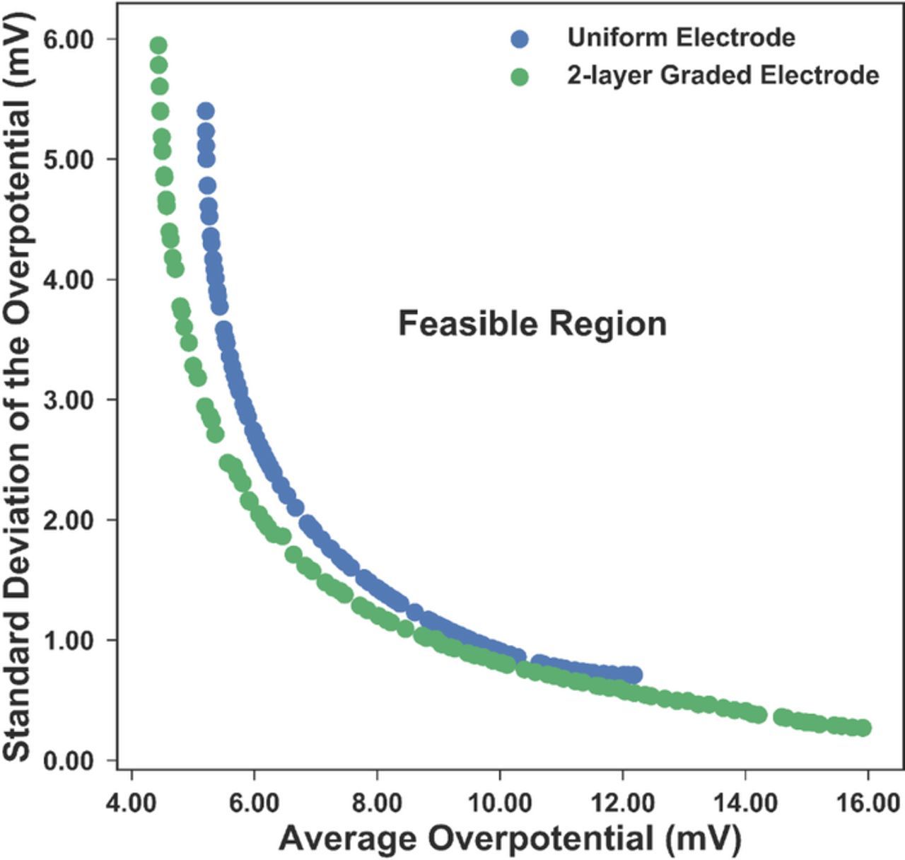
**Figure 8.** The Pareto front plot for minimizing the standard deviation and the mean of the overpotential. The space above the Pareto front represents the feasible region of this problem. Each dot in the plot is a Pareto-optimal solution from the NSGA-II optimizer.

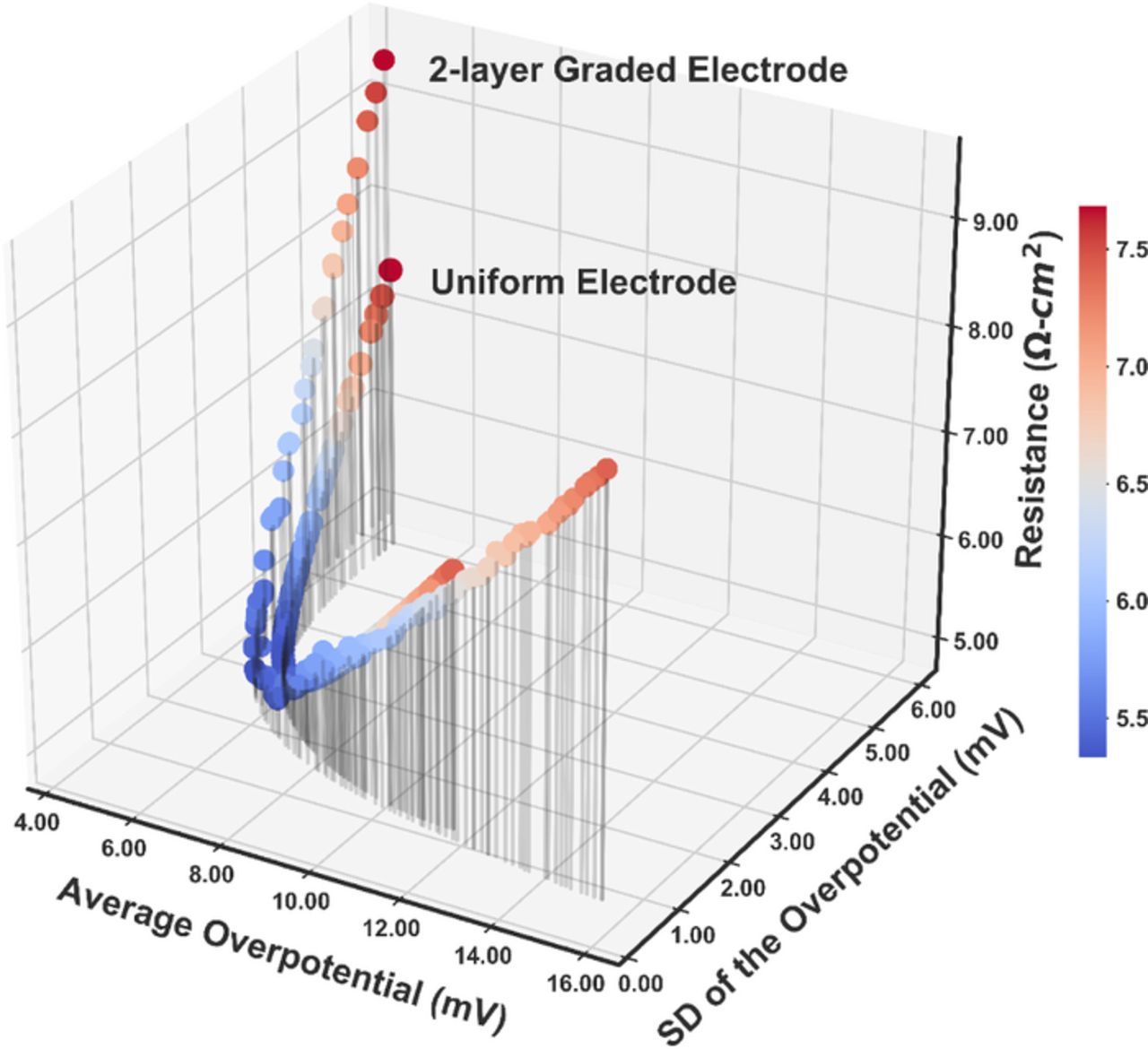
**Figure 9.** The corresponding resistance values for the Pareto-optimal solutions from minimizing both the average and the standard deviation of the overpotential. The resistance is used to help pick the best solution among the Pareto-optimal solutions, which are considered equally good for minimizing both the average and the standard deviation of the overpotential.

Conclusions

In this study, a secondary current distribution model for the battery electrode with Butler-Volmer nonlinear kinetics was used with both the simultaneous and sequential optimization approaches. The design of a thick positive electrode with a uniform porosity and a graded electrode with porosity distribution were explored. An optimal uniform porosity of 0.3435 was predicted consistently by both approaches. For graded electrodes, most of the gain in resistance reduction can be achieved with 2 sub-layers (4.4% reduction in resistance), with the optimal porosity distribution being a higher porosity near the separator and a lower porosity near the current collector. Apart from changing the design variables to optimize the objective function, the simultaneous approach offers the possibility to vary design variables to control the state variables, which cannot be realized directly with the traditional sequential optimization approach. When only one objective function is considered, the advantage of employing graded electrodes is not impressive. However, when more than one objectives are desired, the additional search space introduced by adding the porosity distribution becomes a useful design tool to meet multiple design requirements at the same time. In fact, most of the practical optimization problems in battery design are determined by various design considerations coupled together. A more uniform overpotential distribution can be achieved with the same internal resistance as the optimal uniform electrode using a 2-layer graded structure using the ɛ-constraint method with the simultaneous approach. Thereafter, a multi-objective optimization using the NSGA-II method with the sequential approach was introduced to find the best balance between minimizing the ohmic resistance, the average overpotential, and the standard deviation of the overpotential.

Two open-access free to use executable programs based on the simultaneous approach using the interior point optimizer (IPOPT)²⁴ are provided as a design tool for users to easily adapt for their electrode design problems. The particle size, exchange current density, filler fraction, operation temperature, ionic conductivity, electronic conductivity, electrode thickness, and applied current density can all be customized. They are ready to use with no software installation or programming skill requirement. They can be downloaded directly from the Subramanian group's website (http://depts.washington.edu/maple/Design.html).

As pointed out earlier, the resistance model used did not account for the variance in the electrolyte composition and the time-dependency. This secondary current distribution model captures some key physical processes in the battery yet is still simple enough to be understood, thus it provides a good starting point to explore the application of the simultaneous optimization approach, especially with control of the state variables. However, to be considered for real design applications, a more detailed tertiary current distribution model like the P2D model needs to be used. Applying the simultaneous approach to such a system is extremely challenging. First of all, since all the electroactive species have to be included in the model, the number of design variables will be increased dramatically. Secondly, the number of governing equations also becomes larger. Furthermore, as a consequence of including the transient behaviors, the time-dependent state variables need to be discretized both in time and in space, which will shoot up the number of final "control variables" for the optimizer thereby making it a huge challenge to solve such problems. Results based on P2D model will be reported in the future.

Acknowledgment

Research has been supported by the Assistant Secretary for Energy Efficiency and Renewable Energy, Office of Vehicle Technologies of the U. S. Department of Energy through the Advanced Battery Materials Research (BMR) Program (Battery500 Consortium). This material is based in part upon work supported by the State of Washington through the University of Washington Clean Energy Institute and via funding from the Washington Research Foundation.

ORCID

Yanbo Qi 0000-0001-5852-6011

Venkatasailanathan Ramadesigan 0000-0001-7934-7127

Is There a Benefit in Employing Graded Electrodes for Lithium-Ion Batteries?

Article metrics

Author affiliations

Author notes

ORCID iDs

Dates

Abstract

Choice of the Model: Resistance Model for Battery Electrodes with Nonlinear Kinetics

Optimization Problem Formulation

SOCOLL Method