Abstract
We study the frequency-dependent dielectric polarizability of flexible polyelectrolytes in electrolyte solution by Dissipative Particle Dynamics (DPD) simulations, focusing on the contribution of the electric double layer (EDL) that surrounds the polyelectrolyte. The simulations are based on a recently proposed mesoscopic model that treats the microions in solution at the level of density clouds and solves the corresponding electrokinetic equations using pseudo-particles. The ion diffusivity and the solvent quality are varied systematically. Both factors are found to significantly influence the dielectric properties of the polyelectrolyte: The diffusion of co- and counterions reduces concentration gradients associated with the polarization of the EDL. As a result, the polarizability is a non-monotonic function of the frequency, and in the low-frequency limit, it decreases with increasing ion diffusivity. The solvent quality influences the degree of chain swelling and thus the shape of the EDL. This affects the polarization of the loosely bound co- and counterions in the outer layers of the EDL and leads to a sub-linear scaling of the polarizability with the polyelectrolyte chain length in bad solvent.
Export citation and abstract BibTeX RIS

This is an open access article distributed under the terms of the Creative Commons Attribution 4.0 License (CC BY, http://creativecommons.org/licenses/by/4.0/), which permits unrestricted reuse of the work in any medium, provided the original work is properly cited.
Many applications in bio- and nanotechnology rely on techniques for the controlled handling and manipulation of polyelectrolytes such as DNA molecules.1,2 In particular, one often needs simple, reliable and fast techniques to separate DNA chains according to their size and conformation. Popular separation techniques for charged particles are based on electrophoresis,3 i.e., the drift of charged molecules in an external electric field. Unfortunately, the electrophoretic mobility of freely draining molecules with a Debye layer much smaller than the molecule size is largely independent of the size and shape of the molecule.4 Therefore, alternatives were developed such as gel electrophoresis, where the DNA is pushed through a polymer network by an electric field. However, in such a setup, the viscosity of the background medium is very large by construction, leading to large separation times of 30 min.3,5 Moreover, the separation is only effective for DNA fragments that are not much larger than the mesh size of the gel. It has thus been suggested to instead use dielectrophoresis, i.e. the drift of particles with an (induced) dipole moment in an inhomogeneous, external electric field.6–8 While experiments have demonstrated that dielectrophoresis can indeed be used for separating and controlling DNA molecules, systematic experimental studies of the mechanisms that lead to induced dipole moments in single DNA molecules are still rare. The reason is that the polarizability can only be measured indirectly in experiments, either by ensemble methods9,10 or by measuring escape rates of single DNA molecules from dielectric traps.7
It is well known that several polarization mechanisms compete in DNA or, more general, in polyelectrolytes under the action of an external electric field.11–15 At high frequencies, only the counterions in close vicinity of the chain are rearranged in space, leading to the formation of local dipole moments. Several experimental studies on short stiff DNA fragments9,16–18 have suggested that the resulting polarizability α shows scaling behavior as a function of the length N of the polyelectrolyte, i.e., α∝Nγ, with exponents in the range γ ∼ 2 − 3. The super-linear growth of the polarizability was attributed to correlations between the locally induced dipoles. For flexible chains, a generalization of these scaling laws has been proposed9,19 that takes into account their persistence length λQ. It predicts reduced scaling exponents for chains that are longer than their persistence length L > λQ. In the limit of very long polyelectrolytes, the scaling exponent is predicted to be γ = 1.
At smaller frequencies, the deformation of the EDL around the polyelectrolyte additionally contributes to the total polarizability. For rod-like particles with a Debye length much smaller than the particle size, this contribution has been proposed to scale linearly with the chain length.19 However, in a recent experiment by Regtmeier et al., a sub-linear scaling of the polarizability was reported (γ = 0.4).7
A number of theoretical and simulation studies have been performed in order to understand and verify the scaling behaviors discussed above.20–27 Most of them either consider stiff cylinders,24 rod-like particles20–23 or short weakly-bent chains.25,26 In contrast, in the present work, we focus on the dielectric properties of flexible polyelectrolytes in electrolyte solution. Using coarse-grained computer simulations, we systematically study the scaling of the polarizability with chain length. We find that a transition from super- to sub-linear scaling can be induced by reducing the solvent quality. To understand this transition, we separately investigate the contribution of the inner and outer ion layers surrounding the polyelectrolyte. Furthermore, we analyze the influence of the ion diffusion coefficient on the frequency-dependence of the polarizability and on its limiting behavior at low frequencies.
Our paper is organized as follows: We first describe the details of the proposed mesoscopic simulation model and the procedure used to determine the polarizability of the polyelectrolyte. Then, we present the results for the frequency-dependence of the polarizability, and analyze the role of the ion diffusion coefficient. Finally, we investigate the chain-length dependence of the polarizability for polyelectrolytes for different values of the solvent quality. We close with a brief summary and conclusion.
Simulation Model
All physical quantities in this manuscript are given in reduced Lennard-Jones (LJ) units. This unit system consists of four independent units, i.e., the units of energy  , length σ, time τ and charge e. There is no a priori conversion between the reduced units and SI units since our coarse-grained model has no bottom-up connection to an atomistic system. It is, however, possible to map several model parameters onto a specific microscopic system and estimate the values of the reduced units. In Appendix B, we map our model parameters to the parameters of a polyelectrolyte in a typical ionic solution.
In our simulation model, we consider a single, flexible polyelectrolyte (PE), surrounded by solvent particles that represent the polyelectrolyte solution including co- and counterions. The PE is constructed by connecting N monomers via harmonic bonds. The monomers interact via LJ interactions, whereas the solvent particles have no conservative interactions with other particles. By adjusting the attractive tail of the LJ interaction, the solvent quality can be regulated.28 Every second monomer on the PE is charged, leading to a total charge of Q = N/2 e. The electrolyte contains a corresponding amount of (monovalent) counterions in order to ensure overall charge neutrality, and additional (also monovalent) "salt" ions that further screen the charges and set the Debye length in the solution (λD = 1.78 σ for ρsalt = 0.025 σ− 3). These micro-ions are, however, not modeled as separate explicit particles, but as time-dependent density-fields that generate additional local forces acting on the fluid of solvent particles.
The equations of motion are based on Newton's law for the PE monomers and on the electrokinetic equations for all other constituents. The latter are solved using the Condiff algorithm proposed in earlier work.29,30 In brief, the idea of the Condiff algorithm is to couple two Lagrangian particle-based methods for solving continuum equations, the DPD method for the Navier-Stokes equations and a Langevin method 31 for solving the convection-diffusion equation (the Nernst-Planck equation) describing the time evolution of ion density fields. The fluid flow field is thus represented by DPD particles and the micro-ion fields by a cohort of pseudo-particles that move according to a Langevin equation. The charged PE monomers and the pseudo-particle clouds generate the electric force field that drives their own motion, and the resulting force density field in the ion clouds is transmitted to the fluid of DPD particles. The fluid particles and the PE monomers interact via the DPD equations of motion.32,33 This ensures that the hydrodynamic equations, i.e. the Navier-Stokes equations, are consistently incorporated into the model. The specific model equations can be found in Appendix A, further technical details are discussed in Ref. 30. Here, we use an implementation of the Condiff algorithm in the LAMMPS Molecular Dynamics Software package.34,35
Our motivation for using the ConDiff model rather than an explicit ion model is twofold. First, in the Condiff model, we can implement arbitrary values of the ion diffusion coefficient D in a straightforward manner, since D is a model parameter and not a simulation outcome as in explicit ion models. Second, and even more importantly, explicit ions in coarse-grained simulation models are often too bulky compared to the polymers, and the polymers are too short. We have observed in previous studies36 that this favors a polarization mechanism called volume polarization,37 where ions accumulate outside of the PE under the influence of an electric field (for a more detailed discussion see Appendix C). Here, we wish to study a situation where ions can freely penetrate the PE, which is the case if they are represented by density fields.
In the present work, three different polyelectrolyte models will be investigated which correspond to polyelectrolytes in solvents of different quality:
- PE1:
 (good solvent),
 - PE2: ("bad" solvent)
- PE3: (bad solvent).
The PE1 monomers thus have purely repulsive Weeks-Chandler-Anderson (WCA)- type interactions,39 whereas the monomers in the other two systems experience an additional attractive interaction. In the absence of charges, chains would be expected to collapse ("bad" solvent condition) for values of LJ above LJ/kBT ∼ 0.3.40 However, in the presence of charges, the PE2 chains with LJ/kBT = 0.6 still have a coil shape (see Fig. 1 for a typical simulation snapshot), and only PE3 chains with LJ/kBT = 0.7 are globular.
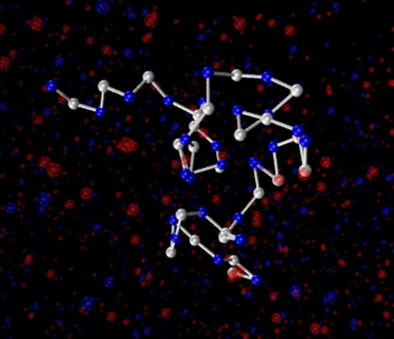
Figure 1. Typical simulation snapshot of model PE2 with N = 50. Uncharged monomers and bonds are drawn in white, charged beads and co-ion pseudo-particles in blue and counterion pseudo-particles in red. The solvent is not shown for visualization purposes. The figure was created using the visualization platform VMD.38
To quantify the conformation differences between these models, we determine the radius of gyration,
![Equation ([1])](https://content.cld.iop.org/journals/1945-7111/166/9/B3194/revision1/d0001.gif)
from the positions ri and center of mass rcom of the polyelectrolyte. The results are shown as a function of chain length N in Fig. 2. Since we will use them to analyze the response of the PEs to an electric AC field, these data were taken in the presence of the same field in the low frequency limit.
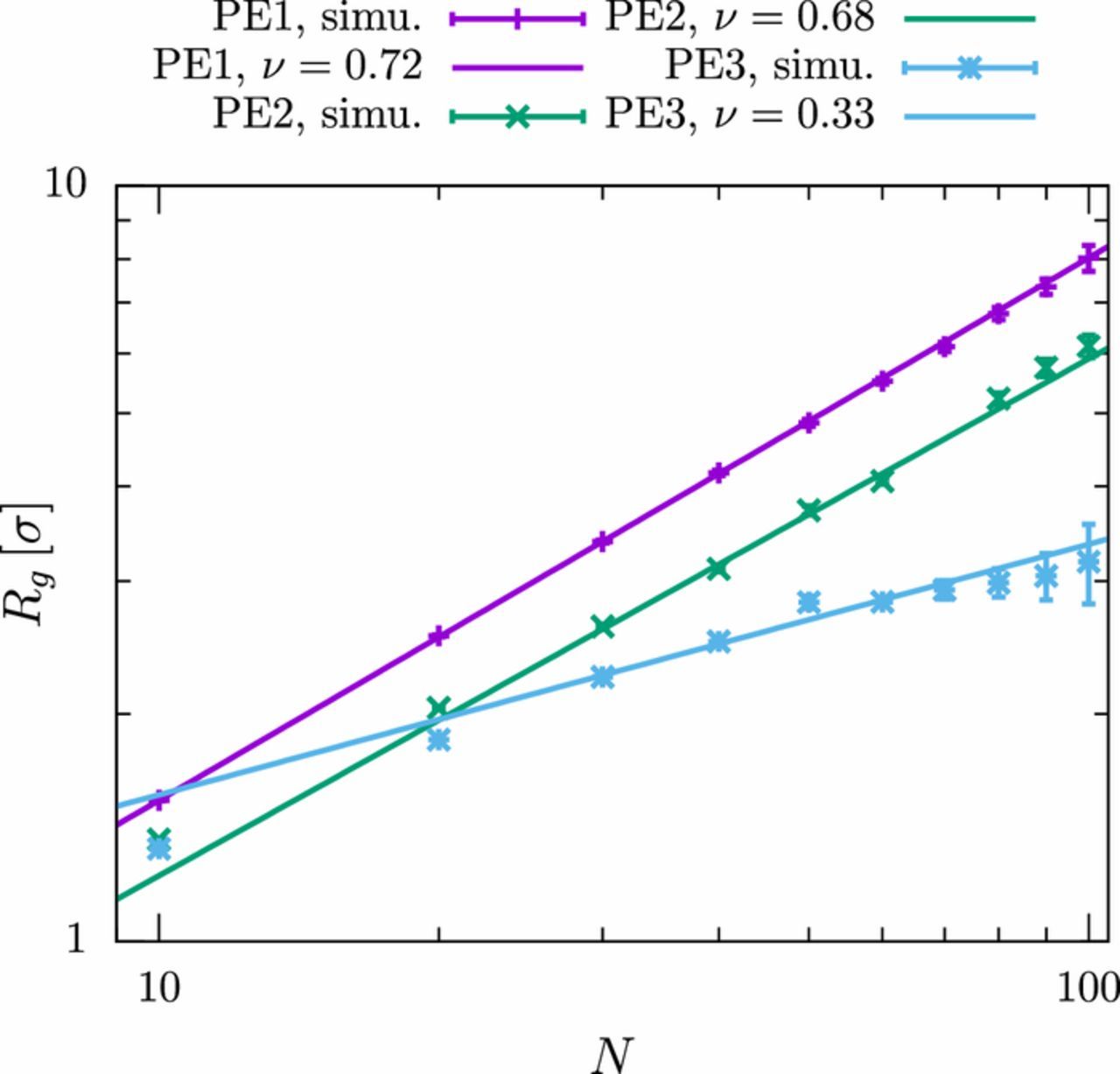
Figure 2. Radius of gyration Rg for polyelectrolytes with different number of monomers N for various solvent qualities (PE1: good solvent, PE2 and PE3: bad solvent). Simulation results are fitted to power laws, Rg∝Nν (the data points for N = 10, 20 were not included in the fit). The values are taken in the presence of an external field with amplitude E0 = 0.5/σe in the low frequency limit (f = 0.002/τ).
As expected, the chain-length dependence of Rg can be fitted by a power-law, Rg∝Nν, where the apparent scaling exponent ν depends on the solvent quality. The observed exponent in the first system PE1, νPE1 = 0.72, is significantly larger than the expected scaling exponent for a polymer with excluded volume interactions in good solvent (ν = 0.588). This can be attributed to the charge-induced repulsion between the beads, which turns out to be important despite the fact that electrostatic interactions are screened by the ions. A comparison to scaling theories for polyelectrolytes in ionic solution shows that we are indeed in the transition region between the rod-like limit (ν = 1) and the ideal chain (ν = 0.5).41 The same holds for the second polyelectrolyte model, PE2. The figure indicates that the chain shrinks slightly when the solvent quality is reduced, however, the scaling exponent for longer chains (N > 30) is not affected significantly.
A completely different picture emerges for polyelectrolyte model PE3. Here, an apparent scaling exponent νPE3 = 0.33 is obtained, which corresponds to a globule structure. The value actually perfectly matches the expected scaling of real, globular polymers in poor solvent. We should note that the power law fit is less convincing for this model than for the other models, indicating that effects of finite chain length are severe in this regime.41
As mentioned above, Fig. 2 shows the scaling behavior of the chains under the action of an external electric field. The values of Rg are slightly larger than those measured under equilibrium conditions (data not shown). This observation can be explained by the deformation of the EDL, which leads to a local increase of the screening length and thus an increased charge-induced repulsion. Interestingly, Zhou and Riehn42 observed the opposite effect for DNA under very strong electric fields. They attribute their findings to a large-scale polarization in the cloud of uncondensed ions that induces attractive interactions between different polarizable subunits of the polyelectrolyte.
To measure the polarizability of the polyelectrolytes, an external field is applied,  , with circular frequency ω0 = 2πf and amplitude E0 = (0.5 /(σe), 0, 0)T. The amplitude is chosen small enough to ensure that the system is still in the linear response regime (see the discussion in Appendix D). The dipole moment is then determined by summing over all pseudo-ions (co- and counterions) within a distance Rmax of the polyelectrolyte,
![Equation ([2])](https://content.cld.iop.org/journals/1945-7111/166/9/B3194/revision1/d0002.gif)
Here, rcoq(t) denotes the center of charge of the polymer. The sum I runs over all ion types (counterions and co-ions), qI = ±e denotes the charge of the corresponding ions, fI the number fI of "real" ions that are represented by one pseudo-ion (fI ≡ 1 in the present work), the sum k runs over all pseudo-ions of type I, and r'k denotes their positions. The distance between pseudo-ions k and the polyelectrolyte is defined as  , where the minimum is taken with respect to all monomer positions ri. The cutoff Rmax was chosen large enough that all charges on the chain are fully screened (Rmax = 4.5 σ ), i.e., the total charge of the EDL,
![Equation ([3])](https://content.cld.iop.org/journals/1945-7111/166/9/B3194/revision1/d0003.gif)
fulfills QEDL = −Q. Hence p(t) does not depend on the reference frame.
In the linear response regime, the Fourier transform of the dipole moment,
![Equation ([4])](https://content.cld.iop.org/journals/1945-7111/166/9/B3194/revision1/d0004.gif)
is zero everywhere (within the noise) except at ω = ω0. (In the nonlinear regime, higher harmonics become important).43 The frequency-dependent polarizability is then defined as
![Equation ([5])](https://content.cld.iop.org/journals/1945-7111/166/9/B3194/revision1/d0005.gif)
In general, the polarizability will be a complex number. The real part α'(ω) = Re[α(ω)] describes the in-phase and lossless response of a dielectric material to an electric field. The imaginary part α''(ω) = Im[α(ω)] (also called the dielectric loss) characterizes the absorption of electric energy of this dielectric material. To investigate the frequency-dependence of the polarizability, we have performed numerical simulations for various AC frequencies ranging from f = 0.002 τ− 1 to f = 1 τ− 1.
The Frequency-Dependence of the Polarizability
Fig. 3 shows the polarizability of polyelectrolyte model PE1 (good solvent) for different frequencies f of the externally applied electric field. One clearly notices a transition from a vanishingly small polarizability at high frequencies to a large polarizability at small frequencies. This phenomenon is also called anomalous dispersion.44 The transition frequency ft ∼ 0.05 τ− 1 = 50 MHz is comparable to the corresponding experimental value (ft, exp = 20 MHz10), indicating that the model captures some of the relevant processes that also determine the polarizability in real systems. Interestingly, the polarizability |α| is not a perfectly monotonous function of the frequency, instead it decreases again as the frequency is further reduced. This non-monotonic behavior can be attributed to a competition of physical processes on two different time scales: The polarization time scale of the uncondensed ions in the EDL, τuc, and the diffusion time scale τd on which the ions diffuse to compensate ion concentration gradients. Such gradients emerge when the EDL deforms in the electric field. Consequentially, we expect the diffusion time scale to be larger than the deformation time scale, and indeed, the transition frequency ft = 0.05 τ− 1 ≈ 1/τuc is well-separated from the frequency fmax = 0.02 τ− 1 ≈ 1/τd below which the polarizability decreases again due to the effect of the ion diffusion. A similar non-monotonous behavior of the polarizability has been observed for nanocolloids.45

Figure 3. Frequency-dependence of the electric polarizability |α| for different ion diffusion constants D. The polyelectrolyte consists of N = 60 monomers (PE1).
The role of the different time scales can be highlighted by analyzing the contribution of different ion layers around the polyelectrolyte to the polarizability. Fig. 4 shows that at high frequencies, only the counterions are polarized. The co-ions contribute at frequencies f < 0.02 τ− 1 = fmax, which is roughly the time scale identified as diffusion time in the previous paragraph. We further note that in the high-frequency regime, the most significant contribution to the polarizability comes from the inner EDL layers. This can be attributed to the fact that ions can only move over small distances in the time of half an AC period, 1/(2f), at high AC frequencies.
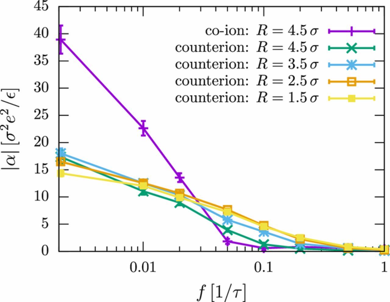
Figure 4. Frequency-dependent contributions of different ion groups to the dielectric polarizability |α|. The different curves show the total contribution of co-ions (purple), and the separate contributions of counterions in layers with a distance R to the polyelectrolyte as indicated. The polyelectrolyte consists of N = 60 monomers (PE1). The ion diffusion coefficient is D = 0.25 σ2/τ.
Fig. 3 also displays the effect of the ion diffusion coefficient D on the polarizability of the polyelectrolyte. Most importantly, it suggests the existence of a cross-over frequency, fc = 0.1 τ− 1, at which different diffusion coefficients result in the same polarizability. For f > fc the system with the largest diffusion coefficient, i.e., the highest ion mobility, has the highest polarizability. In this regime, the ions only have the time to move across the EDL in the time of one AC period, and the amplitude of the resulting ion oscillations is higher if the ions are more mobile. For f < fc, the opposite trend is observed: The polarizability is highest for systems with slowly diffusing ions. In that regime, the diffusion of co-ions results in a significant reduction of the polarizability, and this effect is strongest if the ion diffusion coefficient is large. Interestingly, the polarization depends almost linearly on the inverse diffusion coefficient of the ions (1/D) in the low-frequency limit α(f)|f → 0. To the best of our knowledge, this effect has not yet been discussed in the literature – most studies have focused on the role of the ionic strength of the electrolyte. The reason might be that it is a "second order" effect in some sense: The diffusion of ions is induced by the deformation of the ion cloud which is not incorporated in standard theories like the Maxwell-Wagner relaxation model.46,47
Fig. 5 shows separately the in-phase polarizability and the dielectric loss. The dielectric loss curve α'' is negative, indicating a phase delay of the dielectric response with respect to the phase of the external electric field, and α'' has a minimum around the transition frequency ft. The position of the corresponding minimum in the dielectric loss curve can be used to estimate the diffusion time scale τd, because it coincides with the typical relaxation time of the system. Consistent with our earlier discussion, it depends nearly linearly on the diffusion coefficient of the ions.
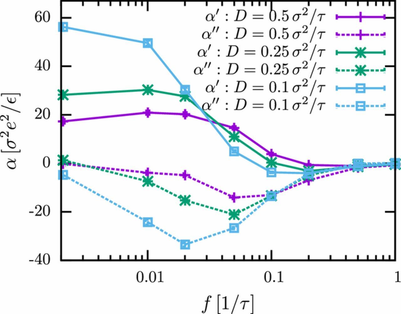
Figure 5. Frequency-dependence of the real part α' and imaginary part α'' of the electric polarizability for different ion diffusion coefficients D. The polyelectrolyte consists of N = 60 monomers (PE1).
The behavior of the real part of the polarizability is similar to that of |α| shown in Fig. 3. It becomes negative close to the transition for small diffusion coefficients, indicating a phase difference ϕ > π/2 between the high-frequency electric field and the response of the EDL. A similar "undershooting" has also been observed in coarse-grained simulation studies of the polarizability of nanocolloids in electrolytes45 with explicit ions. In that case, it could be attributed to the inertia of the ions, implying that it was an unphysical artifact of the simulation model: The time scale of inertia effects,  , was too large in the simulation model since the particle mass m had to be chosen of order unity (in simulation units) for numerical reasons. In the present model, however, the pseudo-ions have no inertia by construction. Thus, we have no obvious explanation for the observed undershooting. Most likely, it is caused by the inertia of the PE monomers.
The influence of the chain length on the frequency-dependence of the polarizability is relatively small, as can be seen in Fig. 6. For the two longer chains, the curves around the transition regime at f ∼ 0.1 τ− 1 almost coincide. This is consistent with the assumption that the AC polarization in that regime is dominated by the periodic motion of ions across the EDL, which has the constant thickness λD independent of the chain length. In the low frequency regime, the polarizability curves feature a maximum, which is located at fmax ∼ 0.01 τ− 1 for chains of length N = 100 and at fmax ∼ 0.02 τ− 1 for chains of length N = 60. Such a behavior would be expected if one assumes the position of the maximum to be determined by the time required for ions to diffuse from one end of the molecule to the other, fmax∝D/R2g (with Rg taken from Fig. 2). However, the same scaling law would predict the maximum to shift to an even higher value for chains of length N = 10, whereas in the simulations, a maximum is found at fmax ∼ 0.01 τ− 1. Hence, other factors seem to be important, at least for short chains.
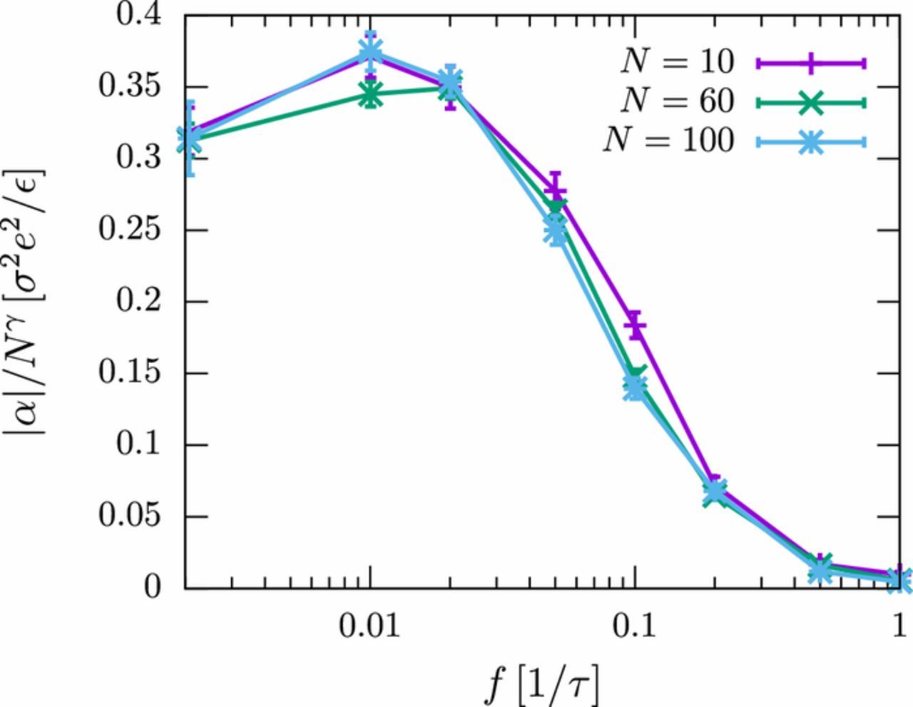
Figure 6. Frequency-dependence of the electric polarizability |α| for different chain lengths N of the polyelectrolyte (PE1). The ion diffusion coefficient is D = 0.25 σ2/τ. The data are rescaled for better visibility by a factor Nγ (γ = 1.1) which is motivated from the analysis in The effect of solvent quality on the polarizability section.
Even though the polyelectrolyte chain length has little influence on the shape of the frequency-dependent polarizability curve α(f), it of course determines the amplitude of the polarizability. This will be discussed in detail in the next section.
The Effect of Solvent Quality on the Polarizability
We will now discuss the scaling of the polarizability with chain length, focusing on the influence of the solvent quality. Fig. 7 shows the polarizability in the low-frequency limit (f = 0.002 τ− 1) as a function of PE chain length for the three polyelectrolyte models PE1, PE2, and PE3. All curves can be described by a scaling law α∝Nγ with different scaling exponents γ. The polyelectrolyte in good solvent (PE1) exhibits a super-linear power law exponent (γ = 1.10 ± 0.02). Since our model has a very small persistence length, λQ ∼ 1 σ ≪ L, this result is in full agreement with the standard scaling theories.9,20 The same also holds for PE2, which has the same polarizability as PE1, as one would expect from the scaling behavior of the radius of gyration (see Fig. 2). The picture, however, fundamentally changes for the third polyelectrolyte model in a bad solvent. Here, the scaling exponent is sub-linear (γ = 0.90 ± 0.01), indicating that the underlying mechanisms are not well described by the standard scaling theories since all of them predict super-linear power laws.

Figure 7. Dependence of the electric polarizability |α| on the chain length N of polyelectrolytes. The simulation results are fitted to power laws, |α|∝Nγ. The frequency of the external field is f = 0.002 τ− 1 and the ion diffusion coefficient is D = 0.25 σ2/τ.
To understand the differences between the systems, we investigate the contribution of different ion layers around the polyelectrolyte (similar to Fig. 4 in the previous section). The results for the polyelectrolytes in good solvent (PE1 model) are shown in Fig. 8. The polarization of all individual layers feature the same, slightly super-linear scaling behavior, which, accordingly, results in the overall super-linear scaling of the polarizability discussed in the previous paragraph (Fig. 7). This is, however, no longer true for polyelectrolytes in a bad solvent (see Fig. 9). While the closest layer displays super-linear scaling with the same exponent as observed in the good solvent, the behavior of the outer layers is characterized by significantly sub-linear exponents (γR = 4.5 σ = 0.50 ± 0.04).
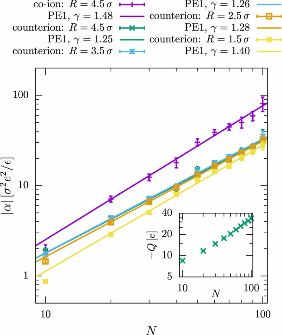
Figure 8. Electric polarizability |α| versus chain length N of the polyelectrolytes (PE1). The different curves show the total contribution of co-ions and the contribution of counterions in layers with a distance of R to the polyelectrolyte. The simulation results are fitted to power laws, |α|∝Nγ (the data points for N = 10, 20 were not included in the fit). The frequency of the external field is f = 0.002 τ− 1 and the ion diffusion coefficient is D = 0.25 σ2/τ. The inset shows the amount of counterions that contribute to polarization of the outer layer (R = 4.5 σ).
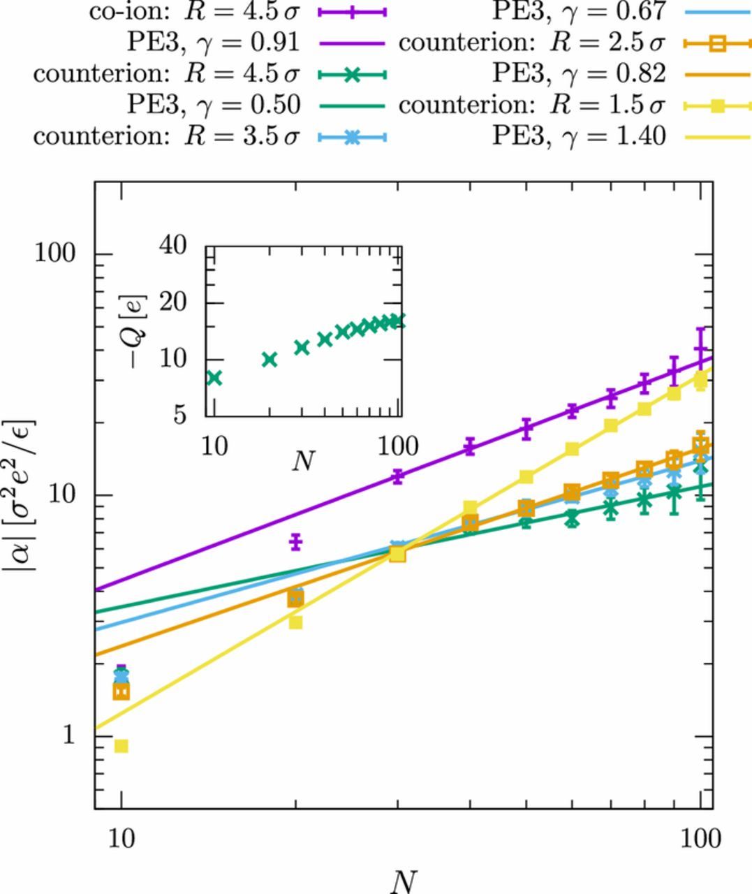
Figure 9. Same as Fig. 8 but for the polyelectrolyte model PE3.
The observations lead to two interesting conclusions: First, the polarizability of the tightly bound counterions in close vicinity to the polyelectrolyte seems to follow a universal scaling behavior, independent of the solvent quality. In previous studies, this contribution was shown to depend on the persistence length λQ,9,19 which was kept approximately constant in this work. Second, the deformation of the outer EDL including the freely associated co- and counterions seems to strongly depend on the conformation of the polyelectrolyte, which varies with varying solvent quality.
We explain this latter observation by the shape of the EDL. We have mentioned previously that the EDL cannot be assumed to be spherical for polyelectrolytes in good solvent. It is more appropriately described by a tube-like structure surrounding the polyelectrolyte. Since the length of the tube increases linearly with the chain length, one expects a linear chain length dependence of the polarization in the limit of a vanishingly small Debye length.19 The situation is, however, different for globular polyelectrolytes in a bad solvent. In that case, the EDL "tube segments" overlap and together form one globule, which is polarized in the presence of an electric field. The amount of counterions in this outer EDL no longer increases linearly with the chain length like in good solvent (Fig. 8, inset), but saturates (Fig. 9, inset), indicating that the charges on the polyelectrolyte are mostly compensated by the tightly bound counterions in the inner EDL. In the outer EDL, a fixed amount of counterions is hence polarized on a length scale proportional to the radius of gyration. This explains the observed sublinear scaling α∝Nγ with γ = 0.5, which is reminiscent of the scaling observed experimentally by Regtmeier et al.7
In our simulations, however, the inner EDL also contributes substantially to the total polarization, and the resulting total effective exponent is much higher, γ ≈ 0.9. In order to rationalize the experimental results based on our simulations, we thus need to identify a mechanism that would suppress the counterion oscillations in the inner EDL in "real" DNA solutions. Such a mechanism is suggested by recent work of Zhao,27 who calculated the polarizability of permeable, homogeneously charged spheres soaked with counterions by numerical solution of the electrokinetic equations in the Stokes limit. He found that the apparent scaling of the polarizability with the total charge (which is proportional to N) depends on the local friction η between sphere and electrolyte inside the sphere. If η is small ("free draining limit"), the scaling is super-linear. If η is very large such that the electrolyte is forced to follow the sphere adiabatically, the scaling is sublinear with an apparent exponent γ ≈ 0.5, consistent with our simulation results for the outer EDL. We therefore conclude that two necessary conditions must be fulfilled in order to obtain sub-linear scaling: The shape of the outer EDL must be globular, and the tightly bound ions in the inner EDL must follow the motion of the chain adiabatically. The second condition is not enforced in our simulations, hence the inner EDL still contributes to the polarizability. In real systems, the motion of tightly bound ions might be suppressed due to an enhanced local friction with the chain. More detailed molecular simulations would be necessary to investigate this possibility.
Conclusions
In this manuscript we have analyzed the influence of two important physical quantities on the frequency-dependent polarizability of polyelectrolytes: The ion diffusivity and solvent quality. We found that increasing the ion diffusion coefficient results in a significant decrease of the polarizability at low frequencies. The effect could be attributed to the fact that the co- and counterion diffusion, in response to the ion concentration gradients associated with the deformation of the EDL, effectively reduces the polarization. In contrast, at high frequencies, the polarizability is determined by the amplitude of ion oscillations across the EDL, which increases with increasing ion diffusivity (i.e., mobility). The two regimes meet at a cross-over frequency where the polarizability is roughly independent of the ion diffusion coefficient.
We should note that an additional dielectric relaxation process with low frequency has been reported in experiments on semidilute polyelectrolyte solutions at low salt concentration,12,15 which was attributed to a transport of tightly bound, condensed, counterions along whole chains.15 This process was not observed in the present simulation, possibly because the salt concentration was too high, or because the Manning parameter of the model is too low (see Appendix B).
The solvent quality influences the scaling behavior of the polarizability with the PE chain length. In good solvent, we recover the super-linear scaling exponents known from the literature. In bad solvent, however, we find that the contribution to the polarizability of the outer layers of the EDL show sub-linear scaling. We attribute this transition to the different conformations of the polyelectrolyte and the associated distinct shapes of the EDL.
Our simulation results suggest an explanation for the experimental findings of Regtmeier et al.,7 who observed sub-linear scaling exponents. In their manuscript they report a Flory scaling exponent of ν = 0.45 ± 0.05 which could indicate that the buffer solution used in the experiments was not a good solvent.
For more quantitative predictions of the polarizability of DNA, it would be necessary to construct more realistic coarse-grained models that also match the persistence length and the Manning parameter of DNA (see Appendix B for details) as well as local mobility differences between tightly and loosely bound ions. Additionally, the physical properties of the surrounding fluid (e.g. Schmidt number) and ions (e.g. size and correlations) have to be matched to the buffer solutions used in experiments. The polarizability of DNA molecules results from a complex interplay of different dynamical processes in the polyelectrolyte and in the ionic solution on different length and time scales. Our study has provided insight into some of these physical mechanisms. We hope that we can thus contribute to a more detailed understanding of the dielectric properties of polyelectrolytes, which will also be useful for devising future separation and manipulation techniques for polyelectrolytes.
Acknowledgment
We thank Burkhard Dünweg for fruitful discussions. This work was funded by the German Science Foundation within project A3 of the SFB TRR 146. Computations were carried out on the Mogon Computing Cluster at ZDV Mainz and the Hazel Hen Computing Cluster at the High Performance Computing Center Stuttgart (HLRS).
ORCID
Friederike Schmid 0000-0002-5536-6718
: Appendix A: The ConDiff Model for Polyelectrolytes
In this appendix, we summarize the equations of motion for PE monomers, DPD solvent particles, and pseudo-particles in the ConDiff algorithm.30 Pseudo-particle and particle positions are denoted r, and velocities v. The total force on the PE monomer i is given by
![Equation ([A1])](https://content.cld.iop.org/journals/1945-7111/166/9/B3194/revision1/d0006.gif)
where the conservative force FCi subsumes the bonded interactions and the LJ interactions between PE monomers
![Equation ([A2])](https://content.cld.iop.org/journals/1945-7111/166/9/B3194/revision1/d0007.gif)
Here, (i ≠ j) runs over all pairs of monomers, and {i, j} over pairs of monomers that are direct neighbors along the chain, such that every pair is counted only once. The vector rij = ri − rj denotes the distance vector between particles i and j. The dissipative and stochastic DPD contribution FDPDi is given by,
![Equation ([A3])](https://content.cld.iop.org/journals/1945-7111/166/9/B3194/revision1/d0008.gif)
where the sum ∑k ≠ i runs over all monomers and solvent particles, eij = rij/|rij| is the unit vector in the direction connecting particle i an j, vij denotes the velocity difference vij = vi − vj, and Wik is a Gaussian distributed random variable with mean zero and correlation  . The friction constant γ and the noise prefactor σ are related via the fluctuation-dissipation relation
  , and likewise, the weight functions fulfill ωD(r) = ωR(r)2. In the present work, we use the weight function
![Equation ([A4])](https://content.cld.iop.org/journals/1945-7111/166/9/B3194/revision1/d0009.gif)
Finally, the electrostatic force, FELi is given by,
![Equation ([A5])](https://content.cld.iop.org/journals/1945-7111/166/9/B3194/revision1/d0010.gif)
where qi is the charge of monomer i, and E is the electric field at the position ri (see below).
The total force on solvent ("electrolyte") particles is given by
![Equation ([A6])](https://content.cld.iop.org/journals/1945-7111/166/9/B3194/revision1/d0011.gif)
where the DPD contribution is calculated as above and ⟨fELfluid⟩i is the share of particle i on the total electrostatic force transmitted to the fluid. Since the hydrodynamic flows – represented by fluid particles – and the ion concentration profiles – represented by pseudo-particles – are allowed to evolve independently, the solvent particles do not carry fixed charges. Instead, the current local electrostatic forces in the pseudo-particle system are transmitted to the solvent particle system in every time step.
Our system contains two types I of micro-ions (co-ions and counterions) with charges qI = ±e. The corresponding ion concentration clouds are taken to evolve according to the Nernst-Planck equation in the flow field vfluid of the fluid particles and the electric field E. They are represented by a cohort of NpseudoI pseudo-ions of type I, which move according to the Langevin equation,
![Equation ([A7])](https://content.cld.iop.org/journals/1945-7111/166/9/B3194/revision1/d0012.gif)
Here, DI denotes the diffusion coefficient of ions I, and we take all diffusion coefficients to be the same here, DI = D. The variable W'i is a Gaussian white noise variable which has the same properties as the variable Wik described above in the DPD paragraph. From the distribution of pseudo-ions, we calculate the concentration profile ρI(r) via
![Equation ([A8])](https://content.cld.iop.org/journals/1945-7111/166/9/B3194/revision1/d0013.gif)
![Equation ([A9])](https://content.cld.iop.org/journals/1945-7111/166/9/B3194/revision1/d0014.gif)
where the sum i runs over all NpseudoI pseudo-particles, fI denotes the (not necessarily integer) number of "real" ions of type I in the system that are represented by one pseudo-ion I. The charges are thus smeared out according to a Gaussian distribution with width α, which eliminates charge fluctuations on smaller scales.
In the limit α → 0 and NpseudoI → ∞ (fI → 0), the above procedure (ConDiff algorithm) would solve the Nernst-Planck equation exactly.31 This corresponds to a mean-field description of the micro-ion clouds where thermal density fluctuations are fully neglected. In practice, the solution is not exact, not only due to the regularization of short-wavelength structures with the parameter α, but also because the number NpseudoI of sampling pseudo-particles is necessarily finite. However, this is not a drawback, but an advantage: The number of pseudo-particles determines the scale of (thermal) statistical noise, which can thus be included in the present algorithm. In order to set the noise scale to a realistic value, one must choose30 fI ≡ 1. This has been done in the present paper.
Having calculated the density profile of ions, one can calculate the total charge density ρC(r) (which includes the contributions of charged PE monomers as well as co- and counterions), solve the Poisson equation for the electrostatic potential ϕ, and derive the electric field E via
![Equation ([A10])](https://content.cld.iop.org/journals/1945-7111/166/9/B3194/revision1/d0015.gif)
![Equation ([A11])](https://content.cld.iop.org/journals/1945-7111/166/9/B3194/revision1/d0016.gif)
Here, we have introduced the Bjerrum length λB = e2/(4π0rkBT) and included the external electric field E(t). As mentioned in the introduction, the Poisson equation is solved on a lattice using the P3M algorithm.48
The ConDiff algorithm involves two communication steps between the DPD system of "fluid particles" and the pseudo-particle system: The transfer of the fluid velocity profile from fluid particles to pseudo-particles, and the transfer of forces from the pseudo-particles to the fluid particles. This is done using a grid with mesh size between 0.9 − 1.1 σ, depending on the box size, and a stencil order of 5 (the same grid is used for the P3M algorithm). Details of the communication procedure can be found in Ref. 30.
This mesoscopic model for polyelectrolytes described above has been implemented in LAMMPS.35 A summary of the model parameters used in our large-scale numerical simulations can be found in Table AI.
Table AI. Summary of the coarse-grained model parameters for the polyelectrolyte (PE) solution, including the list of values used in the present work.
| Parameter explanation | Value | |
|---|---|---|
| kBT | temperature | 1.0 |
| L | box size | 20.0 − 70.0 σ |
| ρDPD | DPD number density | 3.0 σ− 3 |
| γ | DPD friction constant | 5.0 τ/σ2 |
| rc, DPD | DPD cutoff | 1.0 σ |
| D | ConDiff diffusion coefficient | 0.1 − 0.5 σ2/τ |
| ρsalt | salt number density | 0.025 σ− 3 |
| λB | Bjerrum length | 1.0 σ |
| α | size of smeared out charges | 0.5 σ− 1 |
| N | number of monomers | 10 − 100 |
| Q | charge of the polyelectrolyte | N/2 e |
| K | harmonic bond strength | 60 /σ2 |
| r0 | harmonic bond length | 1.0 σ |
| LJ |
LJ interaction strength | 0.6 − 1.0 |
| σLJ | LJ particle diameter | 1.0 σ |
| rc, LJ | LJ cutoff |  |
| E0 | amplitude of external electric field | 0.5 /σe |
: Appendix B: Mapping Reduced Units to SI Units
To determine a realistic mapping between the coarse-grained model studied in this work and a real polyelectrolyte in water, the relevant physical quantities should coincide in both systems, which are in our case the solvent viscosity η, the Debye length λD, and the temperature. The viscosity describes the dynamics of shear waves in the system and is thus an important factor when looking at electrohydrodynamic effects, the Debye length λD determines the length scale on which the electrostatic interactions are screened. These considerations lead to the following mapping from the reduced units system to SI units:
- The viscosity η of the DPD fluid corresponds to 1 mPa · s (the viscosity of water).
- The Debye screening length λD = 1.78 σ corresponds to 3 nm (the approximate screening length of the ionic solution used in Ref. 7.
- The temperature T = /kB corresponds to 295 K.
- As commonly done in coarse-grained polyelectrolyte simulations, we have set the Bjerrum length corresponding to the charge unit e in our model to λB = 1.0 σ (see Table AI). Given the relative permittivity of water at room temperature, r = 80, this also defines the mapping of the charge unit e, which thus corresponds to roughly 1.5 "true" elementary charges.
The results of the mapping can be found in Table BI. The time scale τ corresponds to about 1 ns and the length scale σ is approximately 1.7 nm.
Table BI. Mapping of reduced LJ units to SI units which corresponds to a mapping of the coarse-grained polyelectrolyte to DNA.
| Red. units | SI units |
|---|---|
| σ | 1.69 · 10− 9 m |
|
4.05 · 10− 21 J |
| τ | 9.2 · 10− 10 s |
| e | 2.48 · 10− 19 C |
Comparing our model polyelectrolytes to DNA (see Table BII), we find that one monomer of the coarse-grained polyelectrolyte would correspond to about 5 DNA basepairs (dbp ≈ 0.34 nm). The system considered in this manuscript would thus contain DNA with about 50 − 500 basepairs, which is still smaller than the standardly investigated DNA samples in experiments. Additionally, DNA is much stiffer (the persistence length being roughly 40 nm ∼ 20 σ), and has a much higher charge density. The latter significantly affects the Manning parameter γ0 = λB/lc ,41,49–52 where lc is the distance between neighboring charged monomers. This parameter roughly determines the amount of counterions that will condense on the polyelectrolyte in the absence of salt ions. For values γ0 < 1, very few counterions are expected to condense, while larger values indicate a strong condensation. The Manning parameter for DNA is approximately γ0, DNA = 4.1, and for the polyelectrolyte model used in this work it is γ0, PE = 0.5. These differences will quantitatively affect the values determined for the polarizability. However, since we aim at investigating the response of the uncondensed layer of counterions around the polyelectrolyte, they will not have a significant impact on the qualitative results of this work. We should note that two-state categorization into condensed and "free" counterions is not obvious and much debated when considering ionic solutions with a significant salt concentration.51,53,54 In the present work we therefore use the term "condensed counterions" to denote low-mobility counterions in close vicinity to the polyelectrolyte, without strictly referring to Manning-type condensation.
: Appendix C: Comparison of the ConDiff Model with the Explicit Ion Model
For comparison, we have also performed selected simulations of polyelectrolytes and polymers in electrolytes using a standard explicit ion model.43,45 In this model, ions are "real" DPD-particles that carry a point charge ± e and have WCA-type excluded volume interactions with each other and with the monomers. The other solvent particles have no conservative interactions. Charged monomers also carry point charges.
Fig. C1 shows typical results for the Fourier transform of the polarization px in an electric AC field for the ConDiff model (left panel) and for the explicit ion model (right panel). In the present model, one clearly discerns the expected peak in px(f) at the frequency of the applied field. In the explicit ion model, the peak is absent. The reason for this difference becomes clear if one considers, instead, the polarization of a corresponding neutral polymer in the same AC field (Fig. C2). Here, the trend is opposite: Neutral polymers are not polarized in the ConDiff model, whereas in the explicit ion model, they acquire a negative dipole moment field.
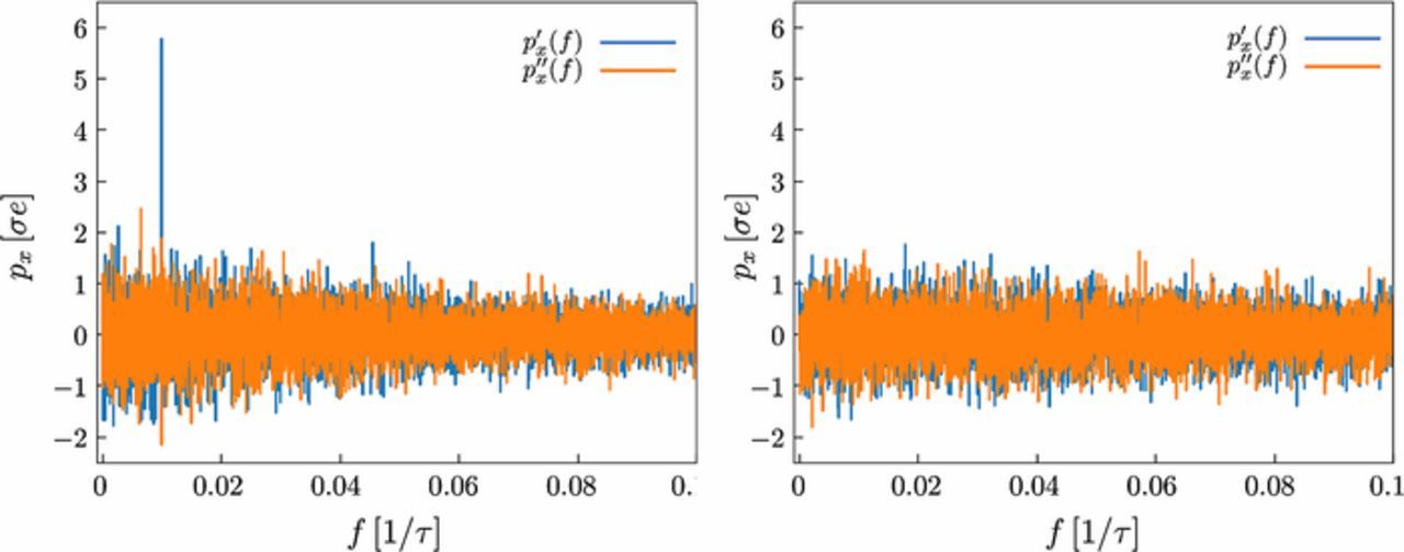
Figure C1. Frequency spectrum of the polarization (real part p'x and imaginary part p''x) for polyelectrolyte model PE1 with N = 21 monomers in an external electric AC field with amplitude E0 = 0.5 /(σe) and frequency f = 0.01 τ− 1. The diffusion coefficient of the ions is D = 0.26 σ2/τ. The left panel shows the results for the ConDiff model, the right panel the results for the explicit ion model.
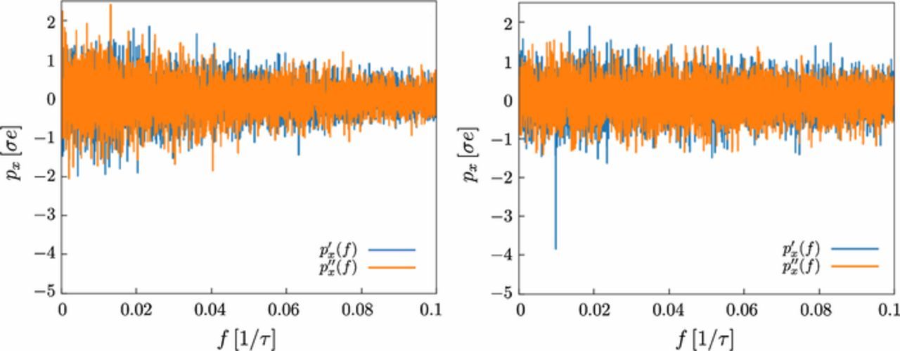
Figure C2. Same as Fig. C1 for a neutral polymer instead of a polyelectrolyte (Q = 0).
The polarization mechanism in this case is an effect which is well-known for colloids, the so-called volume polarization.37,55,56 In an AC field, micro-ions accumulate at the surface of a colloid, since the colloid is an obstacle that blocks their way. This induces a polarization even in uncharged colloids. The resulting dipole moment points in the direction opposite to the applied field. The same effect is also observed in our simulations with explicit ions: Neutral polymers are polarized. In the polyelectrolyte case, the volume polarization and the induced polarization in EDL cancel each other, such that the total polarizability is zero. A similar effect has been described for colloids in Ref. 55.
In real polyelectrolyte solutions, volume polarization may become important if the polymers are very short (oligomers) and/or if the "micro-ions" in the buffer solution are very bulky (e.g., because they are large organic molecules). In general, it can probably be neglected. This is one important motivation to use the ConDiff model in the present study.
: Appendix D: Transition to the Non-Linear Response Regime
In our simulation studies, we must choose a relatively large value for the amplitude of the electric field in order to minimize the statistical error. Nevertheless, we have taken care to stay in the linear response regime. Fig. D1 shows the polarization of a short polyelectrolyte in the low frequency regime as a function of the field amplitude. The dielectric response becomes non-linear for external field amplitudes of E0 > 0.5 /(σe). At the same time, the frequency spectrum of the polarization no longer has the form of Fig. C1, but features additional peaks at frequencies that are multiples 3f0, 5f0, 7f0, ⋅⋅⋅ of the applied frequency f0 (data not shown).
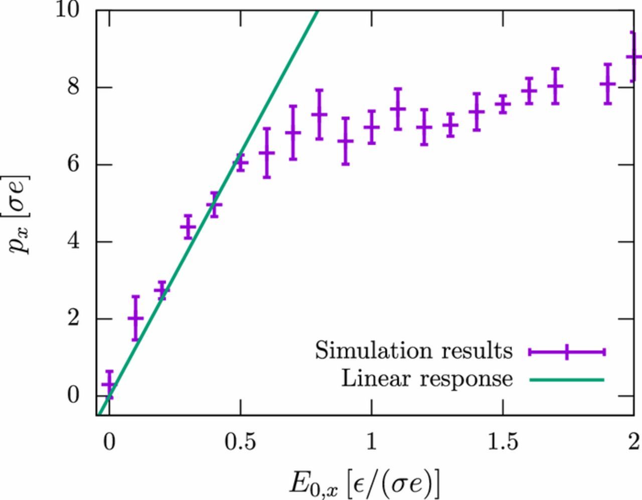
Figure D1. Induced dipole moment px in an external field with amplitude E0 and frequency f = 0.01 τ− 1 for polyelectrolyte model PE1 with N = 21. The diffusion coefficient of the ions is D = 0.26 σ2/τ.