Abstract
A simple and fast diagnostic tool has been developed for analyzing polymer-electrolyte fuel-cell degradation. The tool is based on analyzing changes in polarization curves of a cell over its lifetime. The shape of the polarization-change curve and its sensitivity to oxygen concentration are found to be unique for each degradation pathway based on analysis from a detailed 2-D numerical model of the cell. Using the polarization-change curve methodology, the primary mechanism for degradation (kinetic, ohmic, and/or transport related) can be identified. The technique is applied to two sets of data to explain performance changes after two different cells undergo voltage-cycling accelerated stress test, where it is found that changes are kinetic and then ohmic or transport in nature depending on the cell type. The diagnostic tool provides a simple method for rapid determination of primary degradation mechanisms. Areas for more detailed future investigations are also summarized.
Export citation and abstract BibTeX RIS

This is an open access article distributed under the terms of the Creative Commons Attribution 4.0 License (CC BY, http://creativecommons.org/licenses/by/4.0/), which permits unrestricted reuse of the work in any medium, provided the original work is properly cited.
Polymer-electrolyte fuel cells (PEFCs) have gained increasing interest as an efficient energy-conversion technology.1 However, further improvements in PEFC performance and durability are desired.2 While inventing new materials and cell architectures are crucial in enhancing PEFC performance and durability, developing new diagnostics techniques is equally important to understand the phenomena controlling the cell performance at the beginning of life (BOL) and after degradation, or at end of life (EOL). To study the durability of difference PEFC materials, several accelerated-stress-test (AST) protocols have been developed.3 The ASTs are helpful in simulating and enhancing the underlying stressors that the cell may experience over its lifetime.
Performance degradation during PEFC lifetime can happen due to changes of different cell components via multiple decay mechanisms. These mechanisms result in increases in overpotential due to: a) kinetics, b) ohmic, c) transport, or d) crossover. Some common examples of each of these performance-loss categories include: a) kinetic losses from reduction in catalyst area, which can happen due to sintering, dissolution, contamination, and oxidation;2,4–6 b) ohmic losses from irreversible ionomer degradation or loss in connectivity, thermal effects, and ion contamination;7,8 c) transport losses from changes in hydrophobicity, porosity loss from carbon corrosion, layer delamination, etc.;7,9,10 and d) reactant losses and mixed potentials from increased crossover, which is primarily due to membrane thinning and pinhole formation.11,12 There are a plethora of diagnostic methods to analyze PEFC degradation mechanisms,2,7,12–15 e.g., cyclic volammetry, impedance spectroscopy, oxygen-gain analysis, and X-ray tomography to name a few. While these methods can provide detailed analysis on the reasons for performance degradation during PEFC operation, they can be time and capital expensive. Furthermore, most of the diagnostic methods are suitable to investigate only a single phenomenon in detail. Since the degradation mechanisms are often not known beforehand, pinpointing the cause of performance degradation can become quite cumbersome. Thus, there is a need for relatively quick diagnostic methods to help determine the primary causes of performance loss, and thereby help to down-select and focus more detailed studies. Such a method should be able to provide an easy to understand and physically sound analysis of the experimental data.
PEFC performance at any state (BOL or EOL) is characterized by the polarization curve. Reaction-order and Tafel-slope based diagnostics approaches have been presented in the literature to identify the performance-limiting phenomena.15–17 These methods involve obtaining polarization data at different oxygen concentrations, and observing the change in Tafel slope and/or oxygen reaction order to identify the limiting phenomena. Simple PEFC 1-D models have been used in literature for modeling the limiting cases.15–17 All of these models use first-order Tafel kinetics with an agglomerate model for the ORR. All of the limiting-case solutions assume an isothermal and isobaric cell without bulk diffusion limitations or explicit ionomer film thicknesses in the agglomerate, which are suspected of causing local transport losses in state-of-the-art electrodes.18 For limiting cases, unique reaction orders and Tafel slopes are observed. A summary of the reaction orders and Tafel slopes for different limiting cases is given in Table I.
Table I. Reaction orders and Tafel slopes for different limiting cases.15–17
| Limiting Mechanism | Tafel slope compared to pure kinetic case | Oxygen reaction order |
|---|---|---|
| Kinetic (κm → ∞, Dagg → ∞) | Same | First |
| Kinetic and ohmic (Dagg → ∞) | Double | Half |
| Kinetic and transport (κm → ∞) | Double | First |
| Kinetic, ohmic and transport | Quadruple | half |
While this method is time and cost effective, and provides an easy way to predict the limiting mechanisms, it is based on a simplistic 1-D model of PEFC performance. Furthermore, it cannot necessarily analyze changes between BOL and EOL, and therefore is not as useful for analyzing degradation mechanisms. Recently Perry, et al.7 proposed to use the polarization change curve (PCC) or ΔV curve to identify degradation mechanisms. The ΔV is the difference between BOL and EOL polarization curves. The reaction order of the ΔV curve is determined in the same way as with the polarization curve.15–17 The ΔV curve essentially measures the cell performance degradation, and hence eliminates the effect of parameters which are the same at BOL and EOL. Since the reaction order of the ΔV curve is governed only by the degradation mechanisms, it provides a way for identifying the same.
While the ΔV curve analysis provides an easy to use method for cell diagnostics, the model presented by Perry, et al.7 is based on a simple 0-D cell model. Furthermore, the method has not been validated against experimental data. This article is aimed at investigating the ΔV curve method using a detailed 2-D numerical model of a PEFC. By using a model embedded with detailed PEFC physics, one can analyze the polarization behavior under different limiting mechanisms to develop signatures for changes in physical properties or phenomena. Furthermore, this article aims to validate the interpretations of the model using case studies based on experimental data. The rest of the article is organized as follows: first, a brief overview of the experimental method and operating conditions is presented. Second, the details of the 2-D numerical model used to investigate cell performance are introduced. Next, the limiting cases are shown using the model, followed by analysis of two experimental case studies. Finally, a brief summary of the work is provided.
Experimental
A 12.25 cm2 cell with co-flow triple serpentine channels was used for the degradation study. The cell consists of a SGL25BC (SIGRACET) gas diffusion media on anode and cathode, and the catalyst coated membranes (CCMs) were obtained from Johnson Matthey. The cells are tested at 80C temperature, 150 kPa pressure, and 100% RH. All the tests were run at differential condition (high stoichiometry) to avoid any along-the-channel variations in RH or concentration. For the degradation study, the cell was run through 30,000 voltage cycles (0.6–0.95 V trapezoid).3,19 Table II presents the catalyst loading and other parameters for the two CCMs used in this study.
Table II. BOL parameters for the MEAs used in experimental studies.
| MEA Number | Cathode loading (mg-Pt/cm2) | Anode loading (mg-Pt/cm2) | ECSA (m2/g-Pt) | I/C ratio |
|---|---|---|---|---|
| B1281 | 0.106 | 0.018 | 43 | 1 |
| B1282 | 0.116 | 0.018 | 59 | 1 |
Mathematical Model
A two-dimensional cell model was used to analyze performance at BOL and EOL. The model is based on earlier published frameworks.20–23 Figure 1 shows the schematic of the physical domain for the numerical model. Most of the numerical model is adapted from the COMSOL based model published by Zenyuk, et al.22 The model accounts for reactant diffusion, liquid and gas convection, electronic conduction, water and proton transport through ionomer, and energy transport. While the original model used a double-trap based kinetic model for the oxygen reduction reaction (ORR) in the cathode to account for platinum coverage and changing Tafel slopes, it approximates ORR as a half-order reaction,24 which is contrary to the often measured 0.81 to 1 order in the literature.25–27 Thus, in this work, a Pt-coverage-dependent Tafel-kinetics model modified from Yoon and Weber28 is used instead as detailed below.
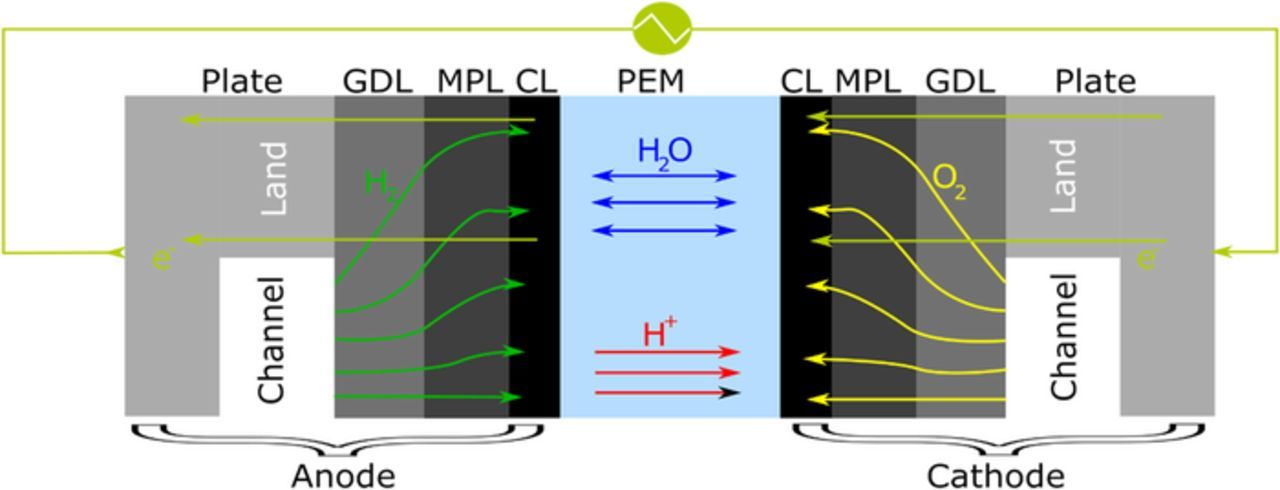
Figure 1. Schematic of the physical domain for the 2-D MEA model.
ORR reaction-kinetics model
For a 0.81 reaction order, the current generation per unit volume in cathode is given as28
![Equation ([1])](https://content.cld.iop.org/journals/1945-7111/165/6/F3007/revision1/d0001.gif)
![Equation ([2])](https://content.cld.iop.org/journals/1945-7111/165/6/F3007/revision1/d0002.gif)
where Av is the specific catalyst area, i0 is the exchange current density,  and
and  are the actual and reference oxygen concentrations, respectively, ϕs is solid phase potential, ϕm is the electrolyte or membrane phase potential, and EOCV is open circuit potential. The PtOH coverage fraction is given as
![Equation ([3])](https://content.cld.iop.org/journals/1945-7111/165/6/F3007/revision1/d0003.gif)
![Equation ([4])](https://content.cld.iop.org/journals/1945-7111/165/6/F3007/revision1/d0004.gif)
where UPtOH = 0.76 V.28,29 The parameters α'a and α'c are adjusted to obtain the Tafel slope doubling at higher current densities; in this work, α'a and α'c are taken to be 0.4 and 0.6, respectively.
Agglomerate model
Most of the agglomerate models in the literature22,30–32 are based on first-order kinetics, which enables an analytical expression for average agglomerate current. With non-first-order kinetics however, the solution has to be modified. In this work, an iterative procedure is used to obtain an average agglomerate current as follows:
- The reaction rate in agglomerate core is obtained from Eq. 1
![Equation ([5])](data:image/png;base64,iVBORw0KGgoAAAANSUhEUgAAAAEAAAABCAQAAAC1HAwCAAAAC0lEQVR42mNkYAAAAAYAAjCB0C8AAAAASUVORK5CYII=)
![Equation ([5])](https://content.cld.iop.org/journals/1945-7111/165/6/F3007/revision1/d0005.gif)
where,  CL is porosity of catalyst layer, and
  is ratio of agglomerate core volume to total agglomerate volume. In terms of agglomerate parameters,
  is expressed as30
![Equation ([6])](https://content.cld.iop.org/journals/1945-7111/165/6/F3007/revision1/d0006.gif)
where, ragg is agglomerate core radius and δagg is the thickness of ionomer film over the core.
- Assuming first-order kinetics, the first approximation of the Thiele modulus (ϕL, 1) and effectiveness factor (Er, 1) are obtained30
![Equation ([7])](https://content.cld.iop.org/journals/1945-7111/165/6/F3007/revision1/d0007.gif)
![Equation ([8])](https://content.cld.iop.org/journals/1945-7111/165/6/F3007/revision1/d0008.gif)
where, M, agg is ionomer volume fraction in agglomerate core, and  is the diffusion coefficient of oxygen in the ionomer.
- Estimate oxygen concentration at surface of agglomerate core assuming first-order reaction30
![Equation ([9])](https://content.cld.iop.org/journals/1945-7111/165/6/F3007/revision1/d0009.gif)
where,  is the oxygen Henry's constant in the ionomer.
![Equation ([10])](https://content.cld.iop.org/journals/1945-7111/165/6/F3007/revision1/d0010.gif)
![Equation ([11])](https://content.cld.iop.org/journals/1945-7111/165/6/F3007/revision1/d0011.gif)
![Equation ([12])](https://content.cld.iop.org/journals/1945-7111/165/6/F3007/revision1/d0012.gif)
![Equation ([13])](https://content.cld.iop.org/journals/1945-7111/165/6/F3007/revision1/d0013.gif)
ΔV analysis
The ΔV depicts the voltage degradation from BOL to EOL at each current, such as:
![Equation ([14])](https://content.cld.iop.org/journals/1945-7111/165/6/F3007/revision1/d0014.gif)
To measure ΔV correctly, VBOL and VEOL should be measured at the same current density. Taking the difference between BOL and the EOL potential ensures that only the effect of the degrading mechanisms is evident. A simple analysis of the ΔV can be performed with a polarization model. A typical 0-D model used for analyzing PEFC polarization curves is given as34
![Equation ([15])](https://content.cld.iop.org/journals/1945-7111/165/6/F3007/revision1/d0015.gif)
Each of the last three terms in the above equation represents a distinct overpotential, as labeled in the equation. Figure 2 shows three simple ΔV curves that are obtained by increasing the overpotential corresponding to one of individual terms in Eq. 15. From this simplistic ΔV analysis it can be seen that each type of overpotential results in a unique shape of the ΔV curve. While this analysis may not hold true with a detailed cell model, it shows the potential of ΔV analysis for identifying the type of overpotentials that have changed, which can then be helpful in determining degradation mechanisms. Other information such oxygen-reaction order can also be analyzed for a better insight on the limiting mechanisms.
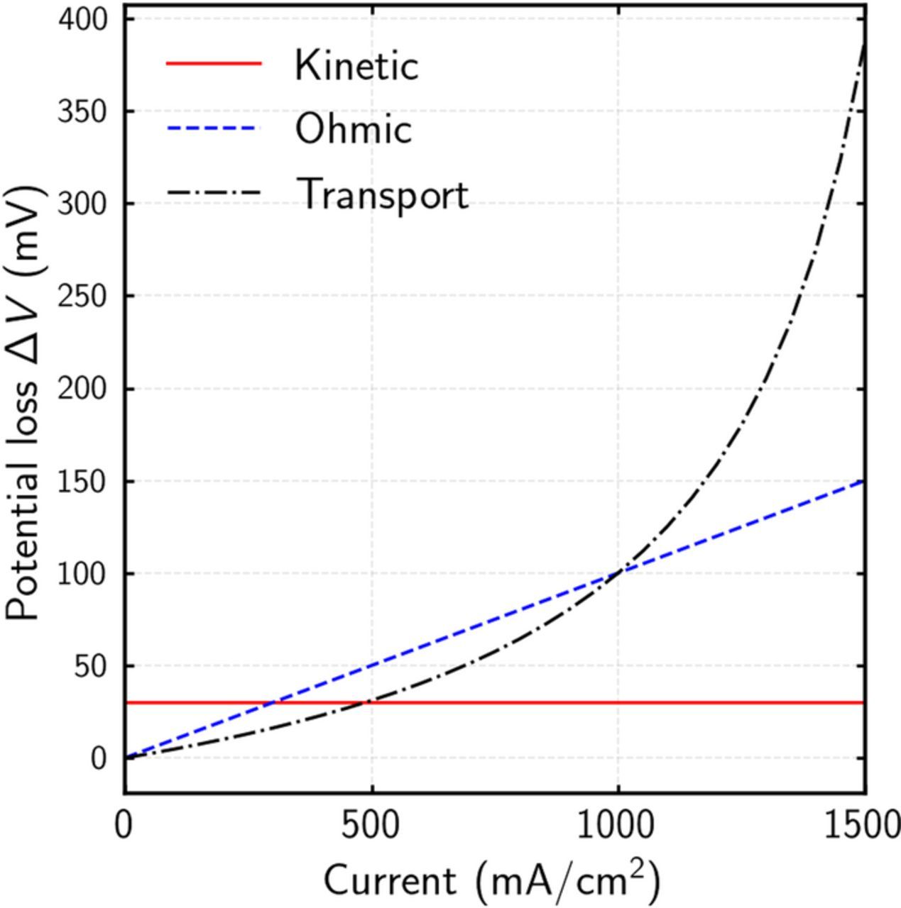
Figure 2. Hypothetical limiting cases of ΔV curve using a simple 0-D polarization model.
Reaction order analysis
To find the reaction order of a cell w.r.t. oxygen concentration at a given potential, cell current at two different oxygen concentrations must be known. Assuming an mth order dependence of cell current density on oxygen concentration, a simple expression for cell current can be given as,
![Equation ([16])](https://content.cld.iop.org/journals/1945-7111/165/6/F3007/revision1/d0016.gif)
Where A(V) is potential dependent constant. For a cell running at a given potential V, cell current at two different oxygen concentrations  , and
, and  , can be given as follows,
![Equation ([17])](https://content.cld.iop.org/journals/1945-7111/165/6/F3007/revision1/d0017.gif)
![Equation ([18])](https://content.cld.iop.org/journals/1945-7111/165/6/F3007/revision1/d0018.gif)
Combining the above two equations results in the following expression:
![Equation ([19])](https://content.cld.iop.org/journals/1945-7111/165/6/F3007/revision1/d0019.gif)
Therefore, if the cell performance is known at any given oxygen concentration, it can be estimated at different oxygen concentrations, provided the reaction order m is known. These estimations can be performed over entire range of operating potential, thereby generating hypothetical polarization curves for a cell.
Results and Discussion
Limiting cases
Using the 2-D cell model describe above, different limiting cases are analyzed. The aim is to compare the findings of a detailed numerical model to the analytical limiting cases presented in the literature (shown in Table I) to confirm their validity or note changes. Different limiting cases were simulated, and the subsequent polarization curves generated for air and half air (10.5% O2 in cathode, which is expected to occur at the exit of a cell assuming a typical stoichiometry of 2). Apart from the numerically estimated pol-curves, hypothetical pol-curves are generated assuming half, and first reaction-order. Thus, assuming either half or first order, one can generate hypothetical curves using Eq. 19 for air from the half-air results:
![Equation ([20])](https://content.cld.iop.org/journals/1945-7111/165/6/F3007/revision1/d0020.gif)
Figure 3 shows the polarization curves for different limiting cases. For each limiting case, a set of phenomenon is limiting, i.e., the potential loss is due to the mentioned limiting mechanisms, and all other mechanisms are neglected. More details on simulation method for each limiting case are given in supplementary information (section 1).
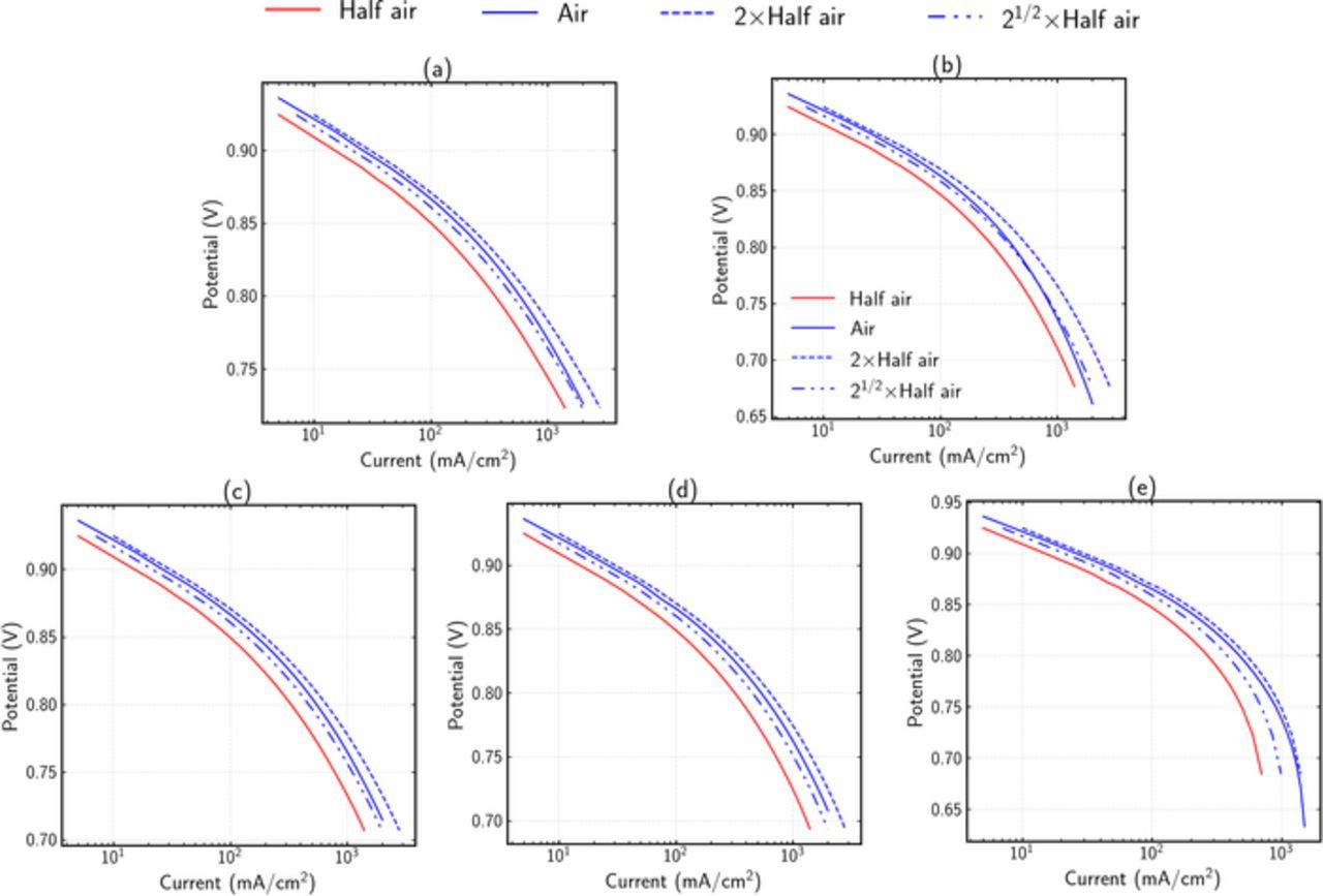
Figure 3. Polarization curves predictions for different limiting cases. Solid lines show numerical results and dashed lines show different reaction-order estimates for air using multiples of the half-air numerical results (see Eq. 20). (a) Kinetics limited case with PtOH coverage dependence, (b) Kinetics and κM, CL limited, (c) Kinetics and Dagg limited, (d) Kinetics and CL diffusivity (DCL) limited, and (e) Kinetics and GDL diffusivity (DGDL) limited.
Figure 3a shows pure kinetic-limited case. It can be observed that the slope changes at higher current densities, which is due to accounting of PtOH coverage, compared to a single slope without PtOH coverage, as shown in supplementary information Fig. 1. Since the slope change can happen due to kinetics as well as other phenomenon, the slope change cannot be attributed distinctively to other mechanisms. The reaction order therefore provides a better way to analyze limiting mechanisms. For the kinetics-limited case, the simulated air polarization curve suggests a reaction order higher than half and close to one, in agreement with the used 0.81 reaction order.
Figure 3b shows the polarization curve with kinetic and ohmic limitations only. At lower current densities, the kinetic losses are dominant and the reaction order is near 0.81. At higher current densities, the ohmic losses also becomes dominant, and the combined reaction order is near one-half. Since the combined order is lower than the pure kinetics-limited case, it can be concluded that the reaction order for a cell limited only by ohmic effects will be even lower than 0.5.
Figure 3c–3e show the polarization curves with kinetics and three different types of transport limitations. Due to dominance of kinetics at lower currents, the curves are similar to kinetics-limited case. At higher currents, it can be observed that the reaction orders are higher than pure kinetics cases. Figure 3c shows a case with significant transport losses and shows a reaction order near 1 for higher current densities. This indicates that the reaction order with oxygen-transport limited cases should be closer to one as expected for diffusional processes (i.e., limiting current). The reaction orders for different mechanisms show reasonable agreement with analytical estimations shown in Table I. At this stage however, the differences between these curves are not significantly differentiated, as most of the polarization curves show coupled effects of kinetics and some other limiting phenomenon.
ΔV Analysis for limiting cases
To clearly identify the effect of each limiting mechanism on reaction order, the effect of each mechanism has to be decoupled. The ΔV analysis provides a means to decouple different limiting mechanisms. To perform the ΔV analysis, two polarization curves are generated: First at BOL with usual cell parameters for the limiting mechanisms such as shown in Figure 3; and a second one at EOL, with the parameters of interest decreased. The difference between these two curves is then solely due to the degradation of parameter of interest.
Using the aforementioned procedure, ΔV curves were obtained at limiting behavior for different mechanisms. Figure 4 shows the ΔV curves for different degradation mechanisms. For a cell with only kinetic related degradation as shown in Figure 4a, the reaction order is ≃ 0.81 as expected. It is also seen that, apart from the initial spike, ΔV is constant for all current densities, which is also predicted by the simple analysis shown in Figure 2. Figure 4b shows the ΔV curves for ohmic degradation of cell. A linear dependence on current density is observed, which is again in agreement with the simple analysis shown in Figure 2. It is also shown that pure ohmic degradation shows a 0th order dependence on oxygen concentration, as the ionomer conductivity is independent of oxygen concentration. Figures 4c–4e show ΔV curves for different oxygen-transport degradations. While Figures 4c–4d for agglomerate diffusivity (Dagg) and catalyst layer (CL) bulk diffusivity (DCL) degradations show a linear behavior, it is only at limiting cases, as shown later in the article. For gas-diffusion layer (GDL) diffusivity (DGDL) degradation (Figure 4e), ΔV has higher magnitude and shows an exponential trend. All of the transport degradation cases show a first-order dependence on oxygen concentration.
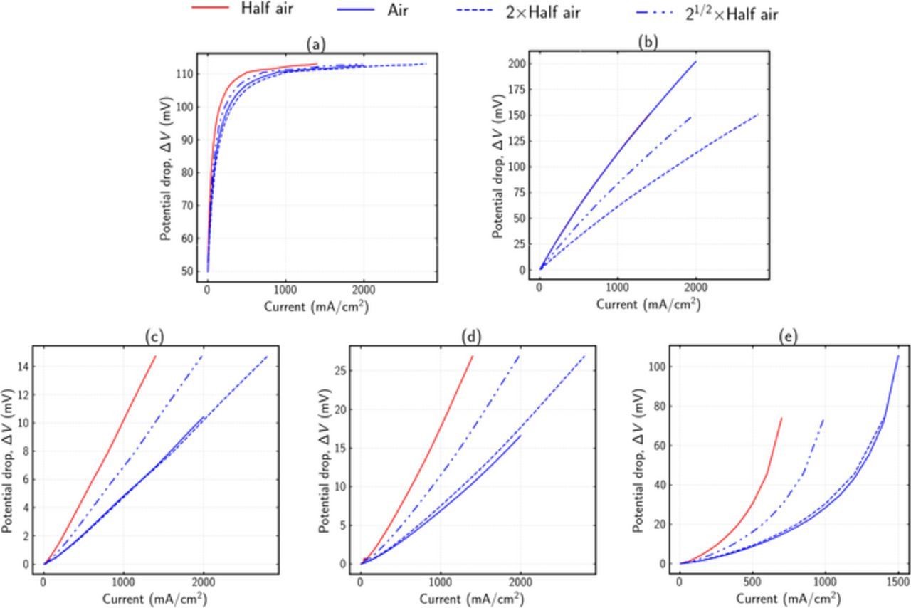
Figure 4. ΔV curves for different limiting cases. Solid lines show numerical results. Dashed lines show different reaction-order estimates for air using multiples of the half-air numerical results. (a) Kinetic degradation. Av, EOL = 0.1Av, BOL, (b) Ohmic degradation. κM, CL, EOL = 0.2κM, CL, BOL, (c) Agglomerate diffusion degradation.  (d) Bulk CL diffusion degradation. DCL, EOL = 0.1DCL, BOL, and (e) Bulk GDL diffusion degradation. DGDL, EOL = 0.2DGDL, BOL.
At this stage, it can be seen that different types of overpotential losses show different behavior, making it possible to distinguish between them. Overall, the simple analysis is shown to be roughly in agreement with the more complex analysis, at least for limiting cases; however, the analysis is still based on limiting cases and may change under real cell conditions where all of the overpotential sources must be considered.
ΔV Analysis under real cell conditions
To understand and identify the degradation mechanisms in a real cell, the analysis tools have to be tested under normal cell operation and parameters as well. So far, the analysis has used limiting-case scenarios where only a single overpotential is encountered and other effects are neglected. For understanding real cell degradation, the ΔV analysis was performed in a similar manner as in the previous section, albeit with a difference: while degradation was simulated for a single mechanism, normal cell parameters were used for the other phenomena to account for all of the coupled overpotentials and physics, i.e., the conductivity, diffusivity, etc. are taken into account for all cases. Details on the different parameters for BOL and EOL simulations are given in supplementary material section 3.
Figure 5 gives the ΔV curves for different limiting cases and combination of limiting cases for normal simulated cells. Purely kinetic degradation was found to show the same behavior as seen with limiting case (Figure 4a) and is therefore not shown here (see supplementary material Fig. 2). One important difference compared to limiting cases is seen in pure ohmic degradation shown in Figure 5a. While the limiting case (Figure 4b) shows a linear shape and zeroth order dependence, degradation at normal cell conditions exhibits exponential behavior at higher current densities, while still remaining linear at lower ones. Similarly, while the oxygen order is near zero at low current densities, it is between half and one at higher ones. The reason for this nonlinear shape and nonzero reaction order at higher current densities is most likely due to the coupling between ohmic and transport effects. At low ionomer conductivity, the ORR occurs closer to the membrane/CL interface, thereby increasing the diffusion length in the CL. This will in turn increase the transport overpotential, resulting in an exponential curve and non-zero order dependence.
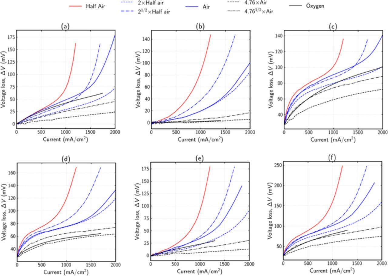
Figure 5. ΔV curves for different limiting cases under normal cell conditions. Solid lines show numerical results. Dashed lines show different reaction-order estimates for air and oxygen using half air and air, respectively (see Eq. 20). (a) Pure ohmic degradation. κM, CL, EOL = 0.2κM, CL, BOL, (b) Pure agglomerate diffusion degradation  (c) Kinetic and ohmic degradation. Av, EOL = 0.25Av, BOL, κM, CL, EOL = 0.2κM, CL, BOL, (d) Kinetic and agglomerate diffusion degradation. Av, EOL = 0.25Av, BOL,
  (e) Ohmic and agglomerate diffusion degradation. κM, CL, EOL = 0.2κM, CL, BOL,
  (f) Kinetic, ohmic and agglomerate diffusion degradation. Combination of (d) and (e).
Figure 5b shows the ΔV curve for pure agglomerate diffusion degradation. Compared to limiting case analysis shown in Figure 4c, it can be seen that the magnitude of ΔV is higher, and the curve is exponential. A first-order dependence on oxygen concentration is seen at normal cell conditions as well.
Figures 5c–5f displays combinations of different property degradations. The following key observations can be made from these figures:
- Ohmic effects show linear behavior at lower current densities, and exponential behavior at higher current densities.
- Reaction order for pure ohmic degradation is near zero at lower current densities, and between half and one at higher current densities.
- Pure transport degradation demonstrates exponential behavior and near first-order dependence for all current densities.
- ΔV for pure oxygen is primarily affected by kinetics degradation.
- For a combination of multiple degradations, the shape and reaction order of the overall curve is a superimposition of individual degradations. The higher the sensitivity of potential to each degradation, the higher should be its superimposed weighting factor.
Table III summarizes the unique signatures of each degradation mechanism. To identify the primary degradation mechanisms(s) in any cell, polarization curves at BOL and EOL must be obtained under at least two oxygen concentrations. ΔV curves can be generated at different oxygen concentrations, and using hypothetical estimation curves, oxygen reaction order can be determined. The shape and reaction order of ΔV curves can be then compared to Table III to identify a single or combination of degradation mechanisms responsible for cell degradation.
Table III. Unique identifiable behavior matrix for different degradation mechanisms.
| Overpotential mechanism |  shape shape |
 order vs oxygen order vs oxygen |
|---|---|---|
| Kinetic degradation | Constant | 1 |
| ohmic degradation | Linear at low current densities Exponential at high current densities | 0 at low current densities ½ to 1 at high current densities |
| Transport degradation | Exponential | 1 |
Case studies using the ΔV diagnostic tool
To examine the applicability of the ΔV diagnostics method, two cells that were subjected to AST protocols are used as examples here. The two cells underwent a voltage-cycling AST for 30,000 cycles and were tested at different oxygen concentrations as described in the Experimental section above. Figure 6 shows the ΔV analysis for one of the cells (B1281), and validation against polarization curves at BOL and EOL. To understand cell degradation and performance at EOL, the experimental ΔV curve can be analyzed. Figure 6a shows the ΔV curved obtained from the experimental BOL and EOL curves. A minor voltage gain was observed at lower current densities using pure oxygen, signifying an increase in catalyst activity, which is likely due to better conditioning of cell after operation. Half-air and air curves show an exponential profile, and for the most part first-order dependence on oxygen concentration. Overall, the degradation appears to be due to change in kinetics and transport losses, which is consistent with the cell AST.
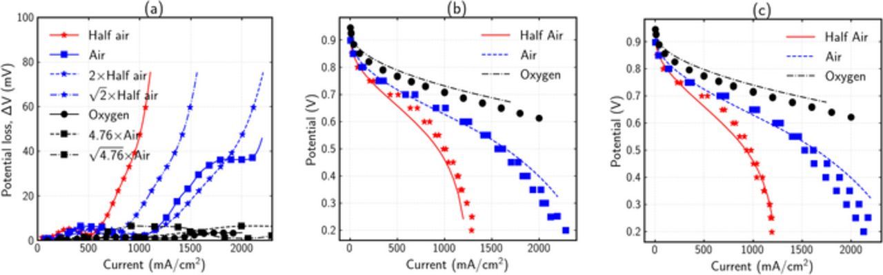
Figure 6. Analysis of cell polarization curves using ΔV analysis for B1281 cell. (a) Experimental ΔV curves at three different oxygen concentrations, (b) Experimental (points) polarization curve at BOL and numerical model (lines) estimates, (c) Experimental (points) polarization curve at EOL and numerical model (lines) results obtained by decreasing only the kinetics and transport parameters relative to BOL.
To determine if the conclusions from this simple ΔV analysis are correct, the experimental curves are also analyzed using the complete cell model. First, the 2-D MEA model parameters such as porosity and agglomerate properties were adjusted to get the best fit to the experimental data. The parameters are fitted using a hit and trial method, where the trend of the pol-curve with each parameter is identified, and an optimum value is selected. While this method may not result in the best fit which can be obtained by methods such as least square fit, it yields a reasonable fit in a minimal amount of time. The cell parameters for best fit at BOL are given in supplementary material section 4. Figure 6b shows the experimental and best fit numerical polarization curves at BOL conditions for different oxygen concentrations. To mimic the likely degradation effects, the kinetic and transport parameters in the fitted BOL model were degraded to obtain the EOL polarization-curve estimations (Supplementary material, Table V). Figure 6c shows the comparison of experimental data and numerical estimates at EOL for different oxygen concentrations. It can be observed that the model agrees well with the experimental results. It must be noted that the EOL numerical results are not obtained by fitting multiple parameters, but by simply changing the kinetics and transport parameters from BOL, as predicted by the ΔV analysis.
Similar analysis was done on another cell, B1282. Figure 7 shows the ΔV analysis and modeling results. Figure 7a shows the experimental ΔV curves at different oxygen concentrations. The potential loss for pure oxygen indicates a significant reduction in catalyst area. The reaction order is between half and one, indicating contribution of ohmic degradation. Since the order is consistently near half for all currents, and does not approach one even at high currents, it can be concluded that transport resistances are not significant. The fitted numerical polarization curves at BOL are shown in Figure 7b. Cell parameters for the best fit are given in supplementary information Table IV. By degrading only kinetic and ohmic parameters in the fitted BOL model, a reasonably good agreement is obtained with EOL polarization curves as shown in Figure 7c. The ability to predict degradation mechanisms and match EOL performance demonstrates the validity of the simple ΔV analysis tool. The ΔVobservations from the two cells can be further corroborated by knowledge of their manufacturing. B1281 used an annealed Pt catalyst which is expected to be stable under the AST,35 therefore showing minimal catalyst loss. The transport loss can be explained by an increase in flooding after the AST. B1282 uses a de-alloyed PtNi catalyst, which is less stable than annealed Pt, thereby resulting in higher kinetics degradation. Furthermore, it is suspected that Ni can dissolve in the low equivalent-weight membranes (EW-850) and move into the ionomer phase in the cell,36,37 thereby adversely impacting the ionic conductivity. Such a phenomenon can explain the ohmic losses in B1282. This effect has not been observed with pure Pt, and therefore does not cause any ohmic losses in B1281.
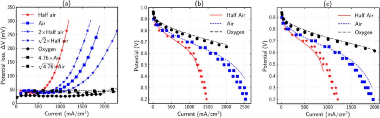
Figure 7. Analysis and validation of cell polarization curves using ΔV analysis for B1282 cell. (a) Experimental ΔV curves at three different oxygen concentrations, (b) Experimental (points) polarization curve and numerical (lines) model results at (b) BOL and (c) EOL. The EOL model results were obtained by degrading only the kinetic and ohmic parameters in the fitted BOL model.
These two case studies demonstrate that ΔV analysis can be a useful and fast tool to analyze fuel-cell performance and identify what types of overpotentials are changing. Since polarization data is routinely collected, this simple analysis does not place any extra burden in terms of cost or time. An overall understanding of the primary types of degradation can direct the use of more detailed diagnostic tools to understand the physical reasons behind the degradations. Although the ΔV analysis is a reliable and fast tool for degradation analysis, it cannot necessarily be used to distinguish between different sources of same types of overpotential degradations. For example, while the analysis can predict transport degradations, it cannot identify if it is due to a collapse in porous structure or due to flooding. Furthermore, it cannot necessarily estimate the location of degradation, i.e. if they are occurring in the GDL, microporous layer, or CL. However, losses that occur external to the CL do exhibit significantly more exponential ΔV curves than internal transport losses, as shown in Fig 4e relative to Figs. 4c and 4d. One can utilize another simple technique, oxygen-gain analysis, to differentiate between transport losses that occur internal and external to the CL.38 Additional insights into actual mechanisms can be gained by performing ΔV analysis with different humidity levels, other gas compositions (e.g., Helox), absolute operating pressures, and/or cell temperatures.
Summary
A simple diagnostic method for analysis of changes in fuel-cell performance has been developed. Using polarization curves taken before and after significant operating time (e.g., at BOL and EOL) or under different operating conditions, polarization curves are compared at different oxygen concentrations to obtain a set of ΔV curves. The shapes of the resulting ΔV curves, and the dependence on oxygen concentration, exhibit unique patterns for different major categories of overpotential (e.g., kinetics, ohmic, transport). A detailed 2-D numerical model of a fuel cell was used to perform limiting-case studies and identify unique signatures for each major category of overpotential. The modeling clearly demonstrated that complex interactions for non-limiting cases result in nonlinear and varying oxygen reaction order and ΔV profiles. The diagnostic tool was demonstrated with BOL and EOL data from two experimental cells where different degradation had occurred and the mathematical model was used to validate the results obtained with the simple diagnostic tool. Currently, the tool can only identify the primary categories of losses (i.e., kinetics, ohmic, and/or transport); it cannot explain the source or exact degradation mechanism. In the future, the analysis can be extended by performing sensitivity with relative humidity, using different gas/oxygen mixtures, or by varying other parameters, in order to get more detailed information on degradation mechanisms.
Acknowledgments
This work was funded under the Fuel Cell Performance and Durability Consortium (FC-PAD), by the Fuel Cell Technologies Office (FCTO), Office of Energy Efficiency and Renewable Energy (EERE), of the U.S. Department of Energy under contract number DE-AC02-05CH11231. The authors thank Iryna Zenyuk at Tufts University for providing the initial COMSOL model and subsequent discussions. The authors would also like to thank Johnson Matthey for providing the MEAs, with special thanks to Brian Theobald and Dash Fongalland for fabricating the catalysts and catalyst layers, respectively.
ORCID
Lalit M. Pant 0000-0002-0432-3902
Adam Z. Weber 0000-0002-7749-1624